Optimal Choice of Crop Insurance: The Case of Winter Barley in France

Abstract

This paper analyzes how the agricultural insurance market is adapting to climate change, particularly as extreme weather events become more frequent and severe. We focus on the optimal decision faced by a risk-averse farmer who wants to insure their crop while making savings. They can choose between a traditional loss-based insurance, index-based insurance or a mix of both. By maximizing the farmer’s CARA utility function, we show that in some cases, a mixed insurance strategy is more advantageous than a single contract. In our model, the farmer insures only part of the crop when the market interest rate is strictly positive. Demand for traditional and index insurance depends on their respective prices. Highly risk-averse farmers prefer traditional insurance. A numerical application to the French agriculture sector indicates that mean spring temperature primarily affects winter barley yield and could therefore be the main indicator for index-based insurance design. Insurance simulations using the theoretical model and the estimated results further illustrate these findings.

1. Introduction

Climate change has become one of the major challenges of the 21st century, particularly for agriculture. The increasing frequency and intensity of extreme weather events (e.g., droughts, floods, heatwaves, and storms) pose significant threats to crop production and yield stability (Beillouin et al. 2020; Lesk et al. 2016). Under such uncertainty, insurance serves as an essential mechanism for transferring and pooling risk. High costs and information asymmetry make it difficult to operate traditional crop insurance sustainably without government subsidies (Leblois and Quirion 2013). Index-based insurance, which relies on weather data or other variables closely correlated with potential losses due to weather events, provides a promising alternative to protect farmers against weather-related risks (Carter et al. 2016; Jensen and Barrett 2017; Miranda and Farrin 2012). It is generally more affordable, while still offering essential protection against extreme weather events (Hess et al. 2005). It is less susceptible to moral hazard or adverse selection (Leblois and Quirion 2013; Lichtenberg and Iglesias 2022) and allows for faster indemnity payments because payouts depend on publicly available data (Alderman and Haque 2006). However, one downside of index insurance is basis risk–the imperfect correlation between the index and actual crop yield (Leblois and Quirion 2013; Lichtenberg and Iglesias 2022).

Index insurance has received substantial attention in agricultural risk management research. To give just a few examples: Barnett et al. (2005); Eltazarov et al. (2023); Miranda (1991) analyze crop insurance based on yield per hectare, Barnett and Mahul (2007); Chantarat et al. (2013); Skees (2008) examine the link between poverty in low-income countries and insurance, and Nguyen et al. (2025) provide a review of existing studies on the development of index-based insurance solutions using satellite data, among many others. Several studies analyze farmers’ insurance choices by maximizing utility functions such as Aina et al. (2024); Cao et al. (2024); Clarke (2016); Hott and Regner (2023); Lichtenberg and Iglesias (2022); Louaas and Picard (2024). However, with the exception of Hott and Regner (2023), these authors primarily focus on a single type of insurance (either index-based or traditional) rather than considering both types simultaneously. Only a few studies analyze both types of insurance jointly (e.g., Lopez and Nkameni (2025); Mensah et al. (2023)). Hott and Regner (2023) add value to the existing literature by treating savings as a substitute for insurance. Nevertheless, the joint optimization of traditional insurance, index insurance, and savings remains largely unexplored. Our study helps to fill this gap by building on the framework proposed by Hott and Regner (2023) and extending it.

In this paper, we examine the decision process between savings, traditional loss-based, and index-based insurance under climatic uncertainty for a risk-averse individual. Assuming homogeneous wealth and heterogeneous intrinsic risk attitudes within the considered population, this study employs a CARA (Constant Absolute Risk Aversion) utility function. Our model extends the theoretical framework of Hott and Regner (2023) by incorporating non-zero interest rates and deriving closed-form optimal strategies for each case. Hott and Regner (2023) proposed a theoretical model for a risk-averse farmer facing a potential loss. They examined the conditions under which the farmer would prefer index insurance over traditional insurance. In some situations, the farmer’s optimal strategy could not be derived explicitly due to the complexity of the calculations. In the original model, the authors use a logarithmic utility function, which is a special case of the CRRA (Constant Relative Risk Aversion) utility family. In the agricultural risk management literature, the CRRA utility function is more commonly used to describe optimal decisions because of wealth changes. However, since wealth is the same for all individuals in our model, using a CARA utility function allows us to model pure heterogeneity in preferences without distortions induced by wealth. Unlike Hott and Regner (2023), we successfully derived closed-form optimal strategies in each scenario thanks to the tractability of the CARA function. We identify the conditions under which the farmer prefers traditional insurance, index insurance, or a combination of the two. The model shows that full insurance occurs only under specific conditions, including a zero market interest rate. Compared to Hott and Regner’s model, we also analyze how optimal strategies change with risk aversion. Greater risk aversion increases demand for traditional insurance, which is not necessarily the case for index-based insurance. The low take-up of index-based insurance can be explained by the fact that premiums exceed what many farmers are willing to pay, consistent with Binswanger-Mkhize (2012)’s findings. We also provide the maximum premium loadings that farmers are willing to pay above actuarially fair premiums in order to cover insurers’ administrative and operational costs. Finally, we apply the model to winter barley in France. Empirical results indicate that mean spring temperature is the most relevant climatic indicator for index-based insurance for winter barley in France. Additionally, simulation results reveal that premium loadings remain a major barrier to adoption.

The remainder of this paper is structured as follows. Section 2 introduces the model framework and its underlying assumptions. Section 3 derives the optimal decisions under single-crop and dual-crop insurance scenarios. Section 4 presents the numerical application of the model to the French agricultural sector. Section 5 discusses the simulation results and their implications for insurance choice. Finally, Appendix A provides the proofs of the optimal decision outcomes.

2. Results

In this section, we develop a theoretical model of a crop farmer, based on Hott and Regner (2023)’s formulation. The model is used to analyze optimal allocations between savings, traditional loss-based insurance, and index-based insurance in the presence of climatic uncertainty.

2.1. Model Assumptions

We consider a farmer who belongs to a group of farmers that own land in the same region and grow a single type of cereal. We assume that all the farmers have heterogeneous intrinsic risk attitudes, but are homogeneous in terms of wealth. We are interested in the decisions made by a risk-averse farmer when facing potential climate-related losses. We assume that they can insure their crop by choosing between two types of insurance contracts: traditional or index insurance. Unlike traditional loss-based insurance which pays compensation when a loss occurs, index insurance is based on realizations of a specific weather parameter measured over a defined period. In this model, the index is triggered by a NatCat event. Therefore, index insurance pays an indemnity only when a NatCat occurs, regardless of whether the farmer actually suffers a loss. Under index insurance, the farmer is exposed to basis risk: the index measurements may not match the farmer’s actual losses. As a result, they may incur losses without receiving any payment or, conversely, receive compensation without experiencing a loss.

At the initial time $t=0$, the farmer has an initial wealth $W_0=1$. They choose s, the amount of savings, and $p\left(\theta \right)$, the amount they are willing to pay for insurance against potential crop losses (where $0\le \theta \le 1$ is the insurance coverage rate). They then consumes the remaining amount $1-s-p\left(\theta \right)$. At $t=1$, the farmer receives the accumulated savings $s(1+r)$, with $r\ge 0$ the interest rate, and obtains a normal agricultural income of 1. However, there is a risk of losing all or part of the harvest. In this model, we assume that the farmer may suffer a crop loss of fixed size $0<l\le 1$ with probability $0<\pi <1$. The insurer pays an indemnity $i\left(\theta \right)$ conditional on the occurrence of the insured event. Therefore, at $t=1$, the farmer’s wealth is $W_1=1+s(1+r)-l+i\left(\theta \right)$. We denote by $0<{\pi }_c<1$ the probability of a NatCat event, and by ${\pi }_h$ (resp. ${\pi }_l$) the probability that the farmer will suffer a loss when there is a NatCat (resp. when there is not). Consequently, the overall probability of a loss can be expressed as $\pi ={\pi }_c{\pi }_h+(1-{\pi }_c){\pi }_l$. Figure 1 illustrates the probability loss.

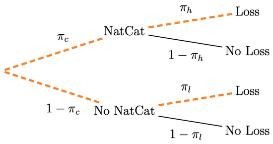
Figure 1. Probability Loss.

Following Hott and Regner (2023), we denote all indices related to traditional insurance with the subscript L, and those related to index insurance with I. In the case of loss-based insurance, the indemnity $i_L$ is triggered only if the farmer experiences a loss. Unlike traditional insurance, index-based insurance pays an indemnity $i_I$ only if a NatCat occurs, regardless of the actual loss.

2.2. Optimal Strategies

We first examine the farmer’s optimal decision when they can choose only one type of insurance (either loss-based insurance or index-based insurance). Then, we analyze the optimal decision for a farmer who purchases both types of insurance. They are assumed to be rational and therefore chooses the optimal level of savings s and insurance coverage rates $\theta$ that maximize their utility U:

$$\underset{s,\theta }{max}\mathbb{E}\left[U(s,\theta )\right]\hspace{1em}\mathrm{subject} \mathrm{to} \mathrm{the} \mathrm{constraints}\hspace{1em}\left\{\begin{array}{c}0\le \theta \le 1\hfill \\ p\left(\theta \right)+s\le 1.\hfill \end{array}\right.$$

The farmer can choose a coverage rate between 0 (no insurance) and 1 (full insurance). The amount saved and the premium paid for insurance cannot exceed their initial wealth.

Compared with Hott and Regner’s model, in which the farmer has a logarithmic utility function, we assume here that the farmer has a Constant Absolute Risk Aversion (CARA) utility function of the form (up to a positive linear transformation) $U\left(x\right)=-{\displaystyle \frac{e^{-\alpha x}}{\alpha }}$ where $\alpha >0$ is the farmer’s absolute risk aversion coefficient. The homogeneity of farmers’ wealth implies that the CARA utility function is appropriate in this setting. Indeed, any difference in behavior toward risk comes solely from intrinsic risk attitudes, not from financial endowments. Moreover, in this model, the farmer’s preferences can be represented by a time-separable intertemporal utility function with a constant discount rate $\rho$. It is the (constant) subjective utility discount rate, also called the rate of time preference. The intertemporal utility function assumes that the farmer derives utility in each period separately, and that intertemporal utility is a weighted sum of the utility levels in the two periods. For simplicity, we set $\rho =r$ throughout the rest of this paper. Unlike Hott and Regner (2023), we consider a nonzero rate and obtain closed-form solutions for optimal savings and insurance for both traditional and index insurance.

2.2.1. One Crop Insurance

We first suppose that the farmer can choose either only a loss-based insurance or only an index insurance.

Traditional loss-based insurance: The indemnity is paid only if the farmer suffers a loss. Therefore, the probability of receiving a payout corresponds to $\pi$, the probability of a loss occurring. The indemnity amount is proportional to the realized loss l and the coverage rate ${\theta }_L$ such that $i_L\left({\theta }_L\right)=l{\theta }_L$. Furthermore, an additional charge factor ${\lambda }_L\ge 0$ is applied to the pure premium to account for administrative costs and other operational expenses. Consequently, the premium paid by the farmer for a coverage rate ${\theta }_L$ is given by:

$$p\left({\theta }_L\right)=(1+{\lambda }_L)\pi l{\theta }_L.$$

The farmer’s intertemporal expected utility under loss-based insurance over the considered period takes the form:

$$\mathbb{E}\left[U_L(s_L,{\theta }_L)\right]=-{\displaystyle \frac{1}{\alpha }}{e}^{-\alpha \left[1-s_L-(1+{\lambda }_L)\pi l{\theta }_L\right]}-{\displaystyle \frac{\pi }{\alpha (1+r)}}{e}^{-\alpha \left(1+s_L(1+r)-l+l{\theta }_L\right)}-{\displaystyle \frac{1-\pi }{\alpha (1+r)}}{e}^{-\alpha \left(1+s_L(1+r)\right)}.$$

(1)

Index insurance: The indemnity is paid only if a NatCat occurs, regardless of whether the farmer actually experiences a loss. Consequently, the probability of receiving a payout is equal to ${\pi }_c$, the probability of a NatCat event. We simplify the indemnity function to an all-or-nothing structure with maximum indemnity $i_I$ (Leblois and Quirion 2013). In contrast to traditional insurance, the indemnity for index insurance will be fixed in advance. In our model, the maximum indemnity is $i_I=l$. As before an additional charge factor ${\lambda }_I\ge 0$ is applied to the pure premium. Therefore, the premium for coverage rate ${\theta }_I$ is given by:

$$p\left({\theta }_I\right)=(1+{\lambda }_I){\pi }_{c}l{\theta }_I.$$

The intertemporal expected utility under index insurance over the considered period is:

$$\mathbb{E}\left[U_I(s_I,{\theta }_I)\right]=-{\displaystyle \frac{1}{\alpha }}{e}^{-\alpha \left[1-s_I-(1+{\lambda }_I){\pi }_{c}l{\theta }_I\right]}-{\displaystyle \frac{{\pi }_c{\pi }_h}{\alpha (1+r)}}{e}^{-\alpha \left[1+s_I(1+r)-l+l{\theta }_I\right]}$$

(2)

$$-{\displaystyle \frac{{\pi }_c(1-{\pi }_h)}{\alpha (1+r)}}{e}^{-\alpha \left[1+s_I(1+r)+l{\theta }_I\right]}-{\displaystyle \frac{(1-{\pi }_c){\pi }_l}{\alpha (1+r)}}{e}^{-\alpha \left[1+s_I(1+r)-l\right]}-{\displaystyle \frac{(1-{\pi }_c)(1-{\pi }_l)}{\alpha (1+r)}}{e}^{-\alpha \left[1+s_I(1+r)\right]}.$$

We denote by $b_L$ and $b_I$ the following boundaries:

$$b_L\left(\alpha \right)={\displaystyle \frac{e^{\alpha l}}{(1+r)(1-\pi +\pi e^{\alpha l})}}\mathrm{and}{b}_I\left(\alpha \right)={\displaystyle \frac{1-{\pi }_h+{\pi }_h{e}^{\alpha l}}{(1+r)(1-\pi +\pi e^{\alpha l})}}.$$

Proposition 1.

Optimal savings and insurance

1. 

If the farmer insures their crops with traditional insurance, the optimal savings and coverage rate are given by:

(a) 

$s_L^{*}={\displaystyle \frac{ln\left(1-\pi +\pi e^{\alpha l}\right)}{\alpha (2+r)}}$ and ${\theta }_L^{*}=0$ if $1+{\lambda }_L\ge b_L\left(\alpha \right)$.

(b) 

$s_L^{*}=-{\displaystyle \frac{(1+{\lambda }_L)\pi l}{2+r}}+{\displaystyle \frac{1}{(2+r)\alpha }}ln\left\{{\displaystyle \frac{1-\pi }{1-(1+r)(1+{\lambda }_L)\pi }}\right\}+{\displaystyle \frac{(1+{\lambda }_L)\pi }{(2+r)\alpha }}ln\left\{{\displaystyle \frac{(1+r)(1+{\lambda }_L)(1-\pi )}{1-(1+r)(1+{\lambda }_L)\pi }}\right\}$ and ${\theta }_L^{*}=1-{\displaystyle \frac{1}{\alpha l}}ln\left\{{\displaystyle \frac{(1+r)(1+{\lambda }_L)(1-\pi )}{1-(1+r)(1+{\lambda }_L)\pi }}\right\}$ if $1+{\lambda }_L<b_L\left(\alpha \right)$.

2. 

If the farmer insures their crops with index insurance, the optimal savings and coverage rate are given by:

(a) 

$s_I^{*}={\displaystyle \frac{ln\left(1-\pi +\pi e^{\alpha l}\right)}{\alpha (2+r)}}$ and ${\theta }_I^{*}=0$ if $1+{\lambda }_I\ge b_I\left(\alpha \right)$.

(b) 

$s_I^{*}={\displaystyle \frac{1}{\alpha (2+r)}}ln\left\{{\displaystyle \frac{(1-{\pi }_c)({\pi }_l{e}^{\alpha l}+1-{\pi }_l)}{1-(1+{\lambda }_I)(1+r){\pi }_c}}\right\}+{\displaystyle \frac{(1+{\lambda }_I){\pi }_c}{\alpha (2+r)}}ln\left\{{\displaystyle \frac{(1+r)(1+{\lambda }_I)(1-{\pi }_c)({\pi }_l{e}^{\alpha l}+1-{\pi }_l)}{[1-(1+{\lambda }_I)(1+r){\pi }_c]({\pi }_h{e}^{\alpha l}+1-{\pi }_h)}}\right\}$ and ${\theta }_I^{*}={\displaystyle \frac{1}{\alpha l}}ln\left\{{\displaystyle \frac{[1-(1+r)(1+{\lambda }_I){\pi }_c]({\pi }_h{e}^{\alpha l}+1-{\pi }_h)}{(1+r)(1+{\lambda }_I)(1-{\pi }_c)({\pi }_l{e}^{\alpha l}+1-{\pi }_l)}}\right\}$ if $1+{\lambda }_I<b_I\left(\alpha \right)$.

On the one hand, excessively high charge factors ${\lambda }_L$, and ${\lambda }_I$ make insurances less attractive (too expensive), prompting the farmer to allocate more to savings and not insure their crop. Hence, if $1+{\lambda }_L\ge b_L\left(\alpha \right)$ and $1+{\lambda }_I\ge b_I\left(\alpha \right)$, the strategy is the same in both cases $s_L^{*}=s_I^{*}={\displaystyle \frac{ln\left(1-\pi +\pi e^{\alpha l}\right)}{\alpha (2+r)}}$ and the farmer doesn’t insure their crop. On the other hand, there would be full traditional insurance (${\theta }_L^{*}=1$) if $r=0$ and ${\lambda }_L=0$. In this case, the farmer finances half the premium via borrowing, leading to negative savings $s_L^{*}=-{\displaystyle \frac{\pi l}{2}}$. If they do not insure their crop, the optimal amount of savings ($s_L^{*}$ when ${\theta }_L^{*}=0$) is higher than it would be if they took out an insurance policy ($s_L^{*}$ when ${\theta }_L^{*}>0$). If the probability that the loss incurred due to a NatCat event is lower than the probability that it is due to an event other than NatCat ${\pi }_h\le {\pi }_l$, then $b_I\left(\alpha \right)\le 1$ and we are never in case 2(b). Hence if ${\pi }_h\le {\pi }_l$, the farmer will not insure their crop even if ${\lambda }_I=0$. In the case of index insurance, the farmer will choose full coverage ${\theta }_I^{*}=1$ only if ${\pi }_h=1$, ${\pi }_l=0$, $r={\lambda }_I=0$. A higher level of r makes insurance less attractive. If the premiums exceed a certain threshold $p\left({\theta }_L^{*}\right)>{\displaystyle \frac{1}{\alpha }}ln\left\{{\displaystyle \frac{1-\pi }{1-(1+r)(1+{\lambda }_L)\pi }}\right\}$ for the loss-based insurance or $p\left({\theta }_I^{*}\right)>{\displaystyle \frac{1}{\alpha }}ln\left\{{\displaystyle \frac{(1-{\pi }_c)({\pi }_l{e}^{\alpha l}+1-{\pi }_l)}{1-(1+{\lambda }_I)(1+r){\pi }_c}}\right\}$ for the index-based insurance, savings will become negative, meaning that the farmer borrows money.

The boundaries $b_L\left(\alpha \right)$ and $b_I\left(\alpha \right)$ (in the case of ${\pi }_h>{\pi }_l$) are increasing functions of $\alpha$, thus more risk-averse farmers are willing to pay higher markups to benefit from insurance coverage. Since ${\partial }_{\alpha }{\theta }_L^{*}\ge 0$, then a higher risk aversion coefficient $\alpha$ increases the overall level of demand for traditional insurance. Note that in the case of a positive demand for index insurance, ${\partial }_{\alpha }{\theta }_I^{*}\ge 0$ for $\alpha \ge {\alpha }^{*}$ and ${\partial }_{\alpha }{\theta }_I^{*}<0$ for $\alpha <{\alpha }^{*}$ with ${\alpha }^{*}$ solution of $ln\left\{{\displaystyle \frac{[1-(1+r)(1+{\lambda }_I){\pi }_c]({\pi }_h{e}^{\alpha l}+1-{\pi }_h)}{(1+r)(1+{\lambda }_I)(1-{\pi }_c)({\pi }_l{e}^{\alpha l}+1-{\pi }_l)}}\right\}={\displaystyle \frac{\alpha l{e}^{\alpha l}({\pi }_h-{\pi }_l)}{({\pi }_h{e}^{\alpha l}+1-{\pi }_h)({\pi }_l{e}^{\alpha l}+1-{\pi }_l)}}$. Hence, a higher risk aversion coefficient (but moderate, remaining below a certain threshold ${\alpha }^{*}$) increases the level of demand for index insurance. As soon as the farmer becomes too risk averse ($\alpha \ge {\alpha }^{*}$), their demand for index insurance will decrease. In particular ${\theta }_I^{*}\to 0$ when $\alpha \to \infty$, which is consistent with Clarke (2016); the optimal index insurance demand is zero for infinitely risk averse individuals.

Direct calculations give the farmer’s utility:

Corollary 1.

Expected utility

1. 

If the farmer insures their crops with traditional insurance, then their maximum expected utility $\mathbb{E}\left[U_L(s_L^{*},{\theta }_L^{*})\right]$ is given by:

$\left\{\begin{array}{cc}-\frac{(2+r)e^{-\alpha }}{\alpha (1+r)}{\left(1-\pi +\pi e^{\alpha l}\right)}^{\frac{1}{2+r}}\hfill & \mathit{if}1+{\lambda }_L\ge b_L\left(\alpha \right),\hfill \\ \frac{-(2+r)e^{-\alpha +\frac{\alpha }{2+r}(1+{\lambda }_L)(1+r)\pi l}{\left[\frac{(1+r)(1+{\lambda }_L)(1-\pi )}{1-(1+r)(1+{\lambda }_L)\pi }\right]}^{\frac{1-(1+r)(1+{\lambda }_L)\pi }{2+r}}}{\alpha (1+r){\left[(1+r)(1+{\lambda }_L)\right]}^{\frac{1}{2+r}}}\hfill & \mathit{otherwise}.\hfill \end{array}\right.$

2. 

If the farmer insures their crops with index insurance, then their maximum expected utility $\mathbb{E}\left[U_L(s_I^{*},{\theta }_I^{*})\right]$ is given by:

$\left\{\begin{array}{cc}-\frac{(2+r)e^{-\alpha }}{\alpha (1+r)}{\left(1-\pi +\pi e^{\alpha l}\right)}^{\frac{1}{2+r}}\hfill & \mathit{if}1+{\lambda }_I\ge b_I\left(\alpha \right),\hfill \\ \frac{-(2+r)e^{-\alpha }{\left[{\pi }_h{e}^{\alpha l}+1-{\pi }_h\right]}^{\frac{1}{2+r}}{\left[\frac{(1+r)(1+{\lambda }_I)(1-{\pi }_c)({\pi }_l{e}^{\alpha l}+1-{\pi }_l)}{[1-(1+r)(1+{\lambda }_I){\pi }_c]({\pi }_h{e}^{\alpha l}+1-{\pi }_h)}\right]}^{\frac{1-(1+r)(1+{\lambda }_I){\pi }_c}{2+r}}}{\alpha (1+r){\left[(1+r)(1+{\lambda }_I)\right]}^{\frac{1}{2+r}}}\hfill & \mathit{otherwise}.\hfill \end{array}\right.$

If ${\pi }_h=1,{\pi }_l=0$ (the loss results solely from a NatCat) and ${\lambda }_I={\lambda }_L=0$, then both insurances give the same expected utility. Since ${\partial }_{{\lambda }_L}\mathbb{E}\left[U_L(s_L^{*},{\theta }_L^{*})\right]<0$ and ${\partial }_{{\lambda }_I}\mathbb{E}\left[U_I(s_I^{*},{\theta }_I^{*})\right]<0$, then an increase in the additional charge factor of a contract reduces its relative attractiveness compared to the other.

2.2.2. Two Crop Insurances

In the previous section, we assumed that the farmer could only choose one type of insurance. We assume now that they insure part of their crop with a traditional insurance and another part with an index insurance. Their expected utility is now:

$$\begin{array}{c}\mathbb{E}\left[U(s,{\theta }_L,{\theta }_I)\right]=-{\displaystyle \frac{1}{\alpha }}{e}^{-\alpha \left[1-s-(1+{\lambda }_L)\pi l{\theta }_L-(1+{\lambda }_I){\pi }_{c}l{\theta }_I\right]}-{\displaystyle \frac{{\pi }_c{\pi }_h}{\alpha (1+r)}}{e}^{-\alpha \left(1+s(1+r)-l+l{\theta }_I+l{\theta }_L\right)}\hfill \\ -{\displaystyle \frac{{\pi }_c(1-{\pi }_h)}{\alpha (1+r)}}{e}^{-\alpha \left(1+s(1+r)+l{\theta }_I\right)}-{\displaystyle \frac{(1-{\pi }_c){\pi }_l}{\alpha (1+r)}}{e}^{-\alpha \left(1+s(1+r)-l+l{\theta }_L\right)}-{\displaystyle \frac{(1-{\pi }_c)(1-{\pi }_l)}{\alpha (1+r)}}{e}^{-\alpha \left(1+s(1+r)\right)}.\hfill \end{array}$$

The farmer chooses the optimal savings amount s and insurance coverage rates ${\theta }_{L,I}$ that maximize their utility U:

$$\underset{s,\theta }{max}\mathbb{E}\left[U(s,{\theta }_L,{\theta }_I)\right]\hspace{1em}\mathrm{s}.\mathrm{t}.\hspace{1em}\left\{\begin{array}{c}{\theta }_L+{\theta }_I\le 1\hfill \\ {\theta }_L,{\theta }_I\ge 0\hfill \\ s+(1+{\lambda }_L)\pi l{\theta }_L+(1+{\lambda }_I){\pi }_{c}l{\theta }_I\le 1.\hfill \end{array}\right.$$

(3)

Proposition 2.

Optimal decision

When the farmer has the option of insuring their crop with two insurance policies, their decision is as follows:

1. 

They do not insure their crop if

$$1+{\lambda }_L\ge b_L\left(\alpha \right)\mathit{and}1+{\lambda }_I\ge b_I\left(\alpha \right).$$

In this case the optimal decision is $(s^{*},{\theta }_L^{*},{\theta }_I^{*})=\left({\displaystyle \frac{ln\left(1-\pi +\pi e^{\alpha l}\right)}{\alpha (2+r)}},0,0\right)$.

2. 

They choose only traditional insurance if

$$1+{\lambda }_L<b_L\left(\alpha \right)\mathit{and}1+{\lambda }_I\ge b_I\left(\alpha \right).$$

In this case the optimal decision is $(s_L^{*},{\theta }_L^{*},0)$ where $s_L^{*}$ and ${\theta }_L^{*}$ are the optimal savings and coverage rates in Proposition 1 (1b).

3. 

They choose only index insurance if

$${\pi }_h>{\pi }_l,1+{\lambda }_L\ge b_L\left(\alpha \right)\mathit{and}1+{\lambda }_I<b_I\left(\alpha \right).$$

In this case the optimal decision is $(s_I^{*},0,{\theta }_I^{*})$ where $s_I^{*}$ and ${\theta }_I^{*}$ are the optimal savings and coverage rates in Proposition 1 (2b).

4. 

The farmer insures their crops with both kinds of insurance if ${\pi }_h>{\pi }_l$,

$$1+{\lambda }_L<b_L\left(\alpha \right),1+{\lambda }_I<b_I\left(\alpha \right)\mathit{and}{\lambda }_I<{\lambda }_L.$$

The optimal savings amount and coverage rates are given by:

$e^{\alpha l(1-{\theta }_L^{*})}={\displaystyle \frac{\left[\pi (1+{\lambda }_L)(1+r)-{\pi }_c(1+{\lambda }_I)(1+r)\right]({\pi }_h-{\pi }_l)+{\pi }_l(1-{\pi }_h)\left[\pi (1+{\lambda }_L)(1+r)-1\right]+\sqrt{\Delta }}{2{\pi }_h{\pi }_l\left[1-\pi (1+{\lambda }_L)(1+r)\right]}},$

$e^{-\alpha l{\theta }_I^{*}}={\displaystyle \frac{\left[{\pi }_l{e}^{\alpha l(1-{\theta }_L^{*})}+1-{\pi }_l\right](1-{\pi }_c)(1+{\lambda }_I)(1+r)}{\left[{\pi }_h{e}^{\alpha l(1-{\theta }_L^{*})}+1-{\pi }_h\right]\left[1-{\pi }_c(1+{\lambda }_I)(1+r)\right]}}$, and

$e^{-\alpha s^{*}(2+r)}={\displaystyle \frac{(1+r)(1+{\lambda }_I)e^{\alpha l\left[(1+{\lambda }_L)\pi {\theta }_L^{*}+((1+{\lambda }_I){\pi }_c-1){\theta }_I^{*}\right]}}{{\pi }_h{e}^{\alpha l(1-{\theta }_L^{*})}+1-{\pi }_h}},$

where

$$\begin{array}{cc}\hfill \Delta & ={\left\{({\pi }_h-{\pi }_l)\left[\pi (1+{\lambda }_L)(1+r)-{\pi }_c(1+{\lambda }_I)(1+r)\right]+{\pi }_l(1-{\pi }_h)\right\}}^2\hfill \\ \hfill & -4\pi {\pi }_c(1+{\lambda }_L)(1+r)(1+{\lambda }_I)(1+r)({\pi }_h-{\pi }_l){\pi }_h(1-{\pi }_l).\hfill \end{array}$$

The farmer will only insure their crop if the insurance is not too expensive. They will choose insurance policies based on their price. The farmer is interested in index insurance if ${\pi }_h>{\pi }_l$. They take out two insurance policies if, in addition, ${\lambda }_I<{\lambda }_L.$

3. Numerical Application

To evaluate the feasibility of parametric insurance, we apply the theoretical model to a real dataset from the French agricultural sector. The objective is to assess whether parametric insurance is more efficient than traditional insurance for a risk-averse farmer. While traditional insurance relies solely on agricultural productivity data, parametric insurance additionally requires meteorological information.

3.1. French Dataset

The constructed dataset comes from two sources. The first source is Agreste (Annual Agricultural Statistics), which provides annual winter barley yields measured in quintals per hectare (q/ha) for each barley-producing region in France from 2010 to 2024. According to Agreste, 93 regions produce winter barley, but only 72 qualify as major producers with more than 2000 hectares under cultivation. Our analysis focuses only on these primary regions, as the full dataset contains missing values for smaller regions and potentially biases the results. Consequently, 72 regions have a complete time series of winter barley yields from 2010 to 2024. Figure 2 shows the changes in winter barley areas for the 2024 harvest compared to 2023 across these regions.

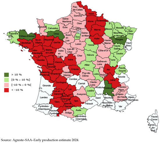
Figure 2. Changes in winter barley areas for the 2024 harvest compared to 2023.

The second source is Datagouv (a French public data platform), which provides monthly regional meteorological indicators since 1950. According to the literature, temperature, precipitation, and solar radiation are the factors that most strongly influence crop production (Hatfield and Prueger 2015; David and Christopher 2007). However, because only a limited number of stations record solar radiation, the sunshine hours index is used to compensate for this deficiency. A total of 3179 weather stations were observed across the 72 barley-producing regions during the study period; 1205 of them continuously recorded monthly precipitation and temperature, which were used to calculate the seasonal weather indicators. In addition, cold- and heat-stress indices are represented by the number of days in a year when the maximum temperature falls below or exceeds a specified threshold. Rainfall intensity is measured by the number of days in a year when cumulative precipitation exceeds a certain threshold.

Regarding winter barley yields across regions, the regional mean production shows substantial variation during the period 2010–2024. Figure 3a shows the mean winter barley yields by region, and Figure 3b presents the average winter barley yield across all regions over time. To define yield losses that are comparable between regions, deviations from each region’s mean yield are used. A negative sign is included so that yield shortfalls (i.e., values below the mean) are expressed as positive yield losses:

$$y_{d,t}=-{\displaystyle \frac{{\widehat{y}}_{d,t}-{\overline{y}}_d}{{\overline{y}}_d}}\times 100\%,$$

where $y_{d,t}$ denotes the percentage negative deviation of the observed yield ${\widehat{y}}_{d,t}$ in region d and year t from its corresponding mean yield ${\overline{y}}_d$.

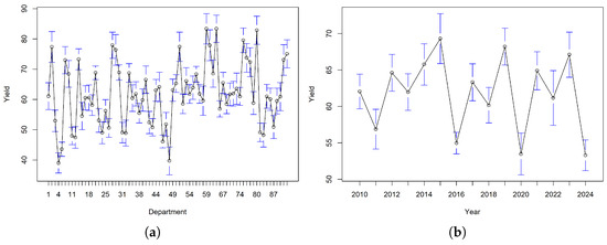
Figure 3. Winter barley yield estimates with 95% confidence intervals by (a) region and (b) year.

Estimating the meteorological index at the regional level requires aggregating station-level observations within each region. A straightforward approach is to take the average of each meteorological index across all stations in a region. However, such an approach neglects the spatial heterogeneity of the stations. A more common method relies on Voronoi (or Thiessen) polygons, which transform point-based observations into planar representations. The Voronoi method partitions the space between neighboring stations into polygons, and the area of each polygon is computed from its vertex coordinates using the Shoelace formula (a discrete form of Green’s theorem). The regional-level index is then estimated by aggregating area-weighted station observations, thereby converting the rasterized data to the regional scale. In total, 16 weather variables are considered to examine their effects on winter barley yield in France. Table 1 presents descriptive statistics for a set of variables with their definition summarized in Table 2.

Table 1. Descriptive statistics of variables.

Variable	Mean	Sd	Min	Pctile[25]	Median	Pctile[75]	Max
Yield	61.81	12.50	21.00	53.00	62.00	70.00	98.00
MeanYield	61.81	10.43	39.01	54.17	61.04	68.58	83.33
DevYield	0.00	11.30	−38.54	−8.20	−1.38	6.79	47.10
NBJRR10	26.97	8.64	7.20	20.50	25.60	31.70	62.00
NBJRR30	2.42	1.98	0.00	1.10	1.80	3.10	15.60
NBJTX0	4.58	5.61	0.00	0.50	2.50	6.40	32.30
NBJTX25	63.06	23.44	10.00	46.87	60.55	79.90	139.60
RR_Aut	239.91	86.92	61.40	177.57	231.40	288.50	660.70
RR_Spr	203.53	81.33	32.40	145.95	194.25	250.70	549.60
RR_Sum	193.10	64.65	63.60	146.07	186.20	230.10	473.90
RR_Win	240.94	86.70	70.00	181.00	228.35	291.65	743.40
INST_Aut	409.14	77.98	0.00	355.96	405.89	463.87	698.90
INST_Spr	574.57	102.58	0.00	510.10	580.93	639.48	831.57
INST_Sum	726.58	109.94	0.00	651.80	721.87	801.01	1023.70
INST_Win	244.89	72.91	0.00	196.58	235.66	281.92	625.57
TM_Aut	12.58	1.55	7.50	11.60	12.50	13.60	17.20
TM_Spr	10.86	1.52	5.40	9.90	11.00	11.90	14.90
TM_Sum	19.26	1.46	15.30	18.20	19.20	20.20	24.30
TM_Win	5.05	1.87	−1.50	3.90	5.20	6.40	9.30

Table 2. Description of variables.

Variable	Definition
Yield	Annual winter barley production by regions (q/ha).
MeanYield	Average winter barley production by regions (q/ha).
DevYield	Negative deviation from the regional mean (%).
NBJRR10/50	Number of days in year with cumulative precipitation ≥10 or ≥50 mm.
NBJTX0/30	Number of days in year with maximum temperature ≤0 °C or ≥30 °C.
RR_Spr/Sum/Aut/Win	Seasonal cumulative precipitation (mm).
INST_Spr/Sum/Aut/Win	Seasonal cumulative sunshine hours.
TM_Spr/Sum/Aut/Win	Seasonal mean temperature (°C).

Figure 4a displays negative deviations over 2010–2024. According to Météo-France, 2018, 2020, 2022, and 2024 rank among the hottest years on record. Consistent with these observations, together with 2011 and 2016, these years exhibit substantial yield losses, as illustrated in Figure 4a. In contrast, the years 2012, 2013, 2015, 2017, and 2019 are associated with comparatively high barley yields, with the negative deviations below zero.

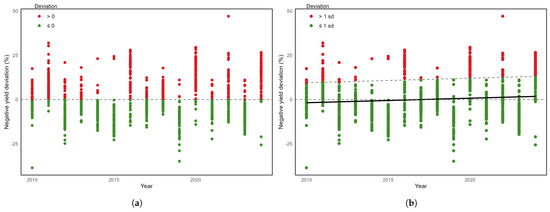
Figure 4. Losses definition with negative deviations of regional yields by (a) mean of the deviations and (b) variation from the trend (red points indicate the losses according to each definition).

Since weather is a complex system with interacting components, correlations between these variables may introduce multicollinearity. As displayed in Figure 5, the weather variables in our dataset show correlations that may need consideration. For example, temperature and sunshine hours are positively correlated, while precipitation and sunshine hours are negatively correlated. Additionally, we observe that low-intensity rainfall occurs throughout the year, whereas high-intensity rain is more likely in spring and autumn. Lastly, we expect positive impacts of low winter temperatures and high summer temperatures on the cold- and heat-stress indices, respectively.

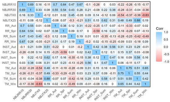
Figure 5. Correlation of standardized seasonal weather indicators.

3.2. Estimation Method

With the complete dataset, we analyze the effects of climatic variables on the negative percentage deviation in winter barley yields. The objective is to determine a suitable weather index that most strongly influences yield outcomes. Given the panel structure of the data, we consider a panel regression model with fixed effects. Individual-fixed effects control for all time-invariant characteristics of each region, while time-fixed effects helpfully capture annual shocks across regions. However, including both individual- and time-fixed effects simultaneously may remove too much variation, leaving only within-individual and within-year variation for model estimation (Kropko and Kubinec 2020). Thus, we use only individual-fixed effects (regions) and account for temporal dynamics (years) via a linear time trend rather than time-fixed effects. This approach may omit short-run shocks but captures gradual long-term changes while preserving sufficient variation to identify the effects of climatic variables. The regression model is given by the following:

$$y_{d,t}={\alpha }_d+\beta X_{d,t}^{st}+\gamma t+u_{d,t},$$

where $y_{d,t}$ denotes the deviation of yield from its regional mean for region d at time t. Along with this, ${\alpha }_d$ denotes region-specific fixed effects, $\gamma t$ captures the linear trend, and $u_{d,t}$ is the error term. $X_{d,t}^{st}$ is a vector of standardized weather variables, which facilitates comparison of coefficients across variables. The standardized weather variables are defined as:

$$X_{d,t}^{st}={\displaystyle \frac{X_{d,t}-\mathbb{E}\left(X_{d,t}\right)}{\sqrt{\mathbb{V}\left(X_{d,t}\right)}}}.$$

We consider three sets of weather variables in the regression analysis. The first estimation includes temperature, precipitation, and sunshine hours, focusing on the effects of deviations from average climatic conditions. In the second and third estimations, temperature and precipitation are replaced, respectively, by the cold- and heat-stress indices, and by rainfall intensity. With these sets of variables, the problem of multicollinearity can be mitigated, as highly correlated variables are separated into distinct sets.

3.3. Estimation Results

Table 3 shows that all seasonal weather conditions are crucial for winter barley yields in France, particularly in winter, spring, and summer. Among the variables considered, temperature has the highest influence on negative yield deviations, followed by precipitation and sunshine duration, consistent with previous findings of Hatfield and Prueger (2015). Specifically, the mean temperature affects yield adversely only when it exceeds or falls below certain thresholds. As shown in Table 1, mean summer temperatures below 25 °C are associated with positive effects on yields, while temperatures above 25 °C are detrimental, as reflected by the positive coefficient for NBJTX25 in the regression. Similarly, temperatures below critical thresholds also reduce yields, as shown by the coefficient of NBJTX0. Although TM_Win has a negative coefficient on the negative yield deviations, the estimates suggest that higher winter temperatures reduce negative deviations and therefore improve yields, consistent with NBJTX0.

Table 3. Fixed-effect with linear trend regressions on weather variables.

Dependent Variable	DevYield
Model	(1)	(2)	(3)
Year	0.742 ***	0.602 ***	0.839 ***
NBJRR10	–	–	−2.957 ***
NBJRR30	–	–	2.219 ***
NBJTX0	–	4.733 ***	–
NBJTX25	–	3.910 ***	–
RR_Spr	1.188 **	3.541 ***	–
RR_Sum	−2.573 ***	−0.525	–
RR_Aut	−1.258 ***	−3.212 ***	–
RR_Win	−1.287 **	−1.737 ***	–
TM_Spr	6.140 ***	–	6.250 ***
TM_Sum	−3.932 ***	–	−2.692 ***
TM_Aut	−0.335	–	−1.148 *
TM_Win	−5.917 ***	–	−6.969 ***
INST_Spr	−2.001 ***	1.365 **	−3.175 ***
INST_Sum	−0.832	−3.288 ***	−0.233
INST_Aut	−1.689 ***	−4.055 ***	−1.603 ***
INST_Win	2.384 ***	1.427 **	3.170 ***
Observations	1080	1080	1080
R2	0.302	0.226	0.285

Significance codes: *** 0.01, ** 0.05, * 0.1.

Precipitation during summer, autumn, and winter positively influences yields within a specific range, even though it has an adverse effect in spring. The estimated results indicate that the number of days with precipitation exceeding 10 mm but not surpassing 30 mm is positively associated with winter barley yields. Furthermore, sunshine hours during spring and summer benefit yields, which contrasts with findings from Germany (Bakker et al. 2005; Hott and Regner 2023). However, an increase in sunshine hours during winter positively influences negative yield deviations, thereby adversely affecting winter barley yields.

Although the explanatory power is limited (low $R^2$), the estimates reveal a statistically significant relationship between weather conditions and winter barley yields in France. Among all variables, mean spring temperature appears to be the most influential factor and is therefore used to calibrate the index-based insurance model.

As a robustness check, time-fixed effects and two-way fixed effects regressions are considered as the alternatives to the baseline model. Table 4 shows that mean spring temperatures consistently appear as the most decisive variables that have the highest effect on the negative yield deviations and remain statistically significant. Table 5 also presents regression estimates for each climatic variable with a baseline model. Although the winter temperature shows the highest $R^2$ value and absolute coefficient, we focus on the mean spring temperature, because its increase is associated with an adverse effect on winter barley yield. These findings suggest that mean spring temperature is a robust variable and that correlations with other variables do not affect the validity of the results.

Table 4. Comparison between regression models.

Dependent Variable	DevYield
Model	Baseline	Time-Fixed Effects	Two-Way Fixed Effects
Year	0.742 ***	–	–
RR_Spr	1.188 **	−0.150	0.538
RR_Sum	−2.573 ***	0.256	1.559 ***
RR_Aut	−1.258 ***	0.293	0.478
RR_Win	−1.287 **	−0.721 *	−1.700 ***
TM_Spr	6.140 ***	5.369 ***	8.561 ***
TM_Sum	−3.932 ***	−1.628 **	6.508 ***
TM_Aut	−0.335	−1.492	−1.739
TM_Win	−5.917 ***	−2.255 ***	−5.479 ***
INST_Spr	−2.001 ***	−1.976 ***	−1.863 ***
INST_Sum	−0.832	−1.417 ***	−2.218 ***
INST_Aut	−1.689 ***	1.352 **	0.854
INST_Win	2.384 ***	0.474	0.279
Observations	1080	1080	1080
R2	0.302	0.059	0.123

Significance codes: *** 0.01, ** 0.05, * 0.1.

Table 5. Fixed-effect with single weather variable and linear trend regression.

Dependent Variable	DevYield
Model	(1)	(2)	(3)	(4)	(5)	(6)	(7)	(8)	(9)
Year	0.256 ***	0.193 **	0.238 ***	0.370 ***	0.240 ***	0.103	0.584 ***	0.248 ***	0.920 ***
RR_Spr	–	1.612 ***	–	–	–	–	–	–	–
RR_Sum	–	–	−0.495	–	–	–	–	–	–
RR_Aut	–	–	–	−2.650 ***	–	–	–	–	–
RR_Win	–	–	–	–	−1.966 ***	–	–	–	–
TM_Spr	–	–	–	–	–	4.076 ***	–	–	–
TM_Sum	–	–	–	–	–	–	−3.784 ***	–	–
TM_Aut	–	–	–	–	–	–	–	0.132	–
TM_Win	–	–	–	–	–	–	–	–	−8.778 ***
Observations	1080	1080	1080	1080	1080	1080	1080	1080	1080
R2	0.01	0.024	0.011	0.047	0.028	0.065	0.036	0.01	0.166

Significance codes: *** 0.01, ** 0.05.

4. Discussion on Insurance Simulation

This section discusses an approach to designing insurance for winter barley yield in France based on the theoretical model presented. Specifically, we determine an optimal threshold for a NatCat event (i.e., the mean spring temperature that triggers index insurance payouts) and compare the calibrated expected utility of a representative farmer under traditional loss-based insurance and index-based insurance to identify the preferable insurance option.

4.1. Simulation of Traditional Insurance

According to Equation (1), simulating traditional loss-based insurance requires the overall probability of loss $\pi$, the loss magnitude l, and the loading factor ${\lambda }_L$ applied to the pure premium. In addition, the parameters for risk aversion $\alpha$, the interest rate r, and the utility discount rate $\rho$ are included in the formulation (with $\rho =r$). Estimating the coefficient of risk aversion typically relies on experimental or survey-based methods. For simplicity, we assume a representative risk-averse farmer with a coefficient of relative risk aversion $\alpha =1$ and set $r=1.7\%$, the current risk-free rate in France.

The parameters $\pi$ and l are derived from crop yield data presented in Section 3. Since the available data provide only annual absolute crop yields or negative deviations from the regional means (the latter calculated additionally), it is necessary to define what constitutes a loss. One possible approach is to classify any negative yield deviation as a loss. However, this would result in a loss probability of about 46%, as reflected in Figure 4a. Thus, a threshold is required to classify only the most extreme negative deviations as losses.

We observe a negative trend in overall crop yields, as reflected in the downward evolution of annual regional mean yields in Figure 3b and the upward trend in deviations from regional means in Figure 4b. With only the mean spring temperature as the explanatory variable, the estimation reveals a linear increasing trend in negative deviation yield of 0.103 per year (see model (6), Table 5). This estimated trend reflects both the decline in yield (increasing negative yield deviations) and the rise in mean spring temperatures (reducing negative yield deviations). We therefore need to disentangle these effects. By minimizing the mean squared error between a linear trend and the negative yield deviations, we estimate a positive trend coefficient of 0.256 (see model (1), Table 5). The difference between these two trend estimates (i.e., 0.153) can be attributed to rising mean spring temperatures each year, in line with the positive coefficient of mean spring temperature on negative yield deviations. The estimated linear trend for mean spring temperature is 0.057. Since we use standardized temperatures (with a standard deviation of 1.52) and a coefficient of 4.076, the induced trend component from mean spring temperature becomes 0.153. Thus, the sum of the two trend components (0.103 and 0.153) equals the trend component in our estimation (i.e., 0.256). Accordingly, losses can be defined as the variation of the negative yield deviations from their estimated trend. As summarized in Table 1, the standard deviation of negative deviations represents about 11.3%. In Figure 4b, approximately 16.7% of the losses exceed the trend line by more than 11.3%, with an average magnitude of about 18.7%. Under this definition, the parameters $\pi$ and l take values of 16.7% and 18.7%, respectively. Increasing the threshold to two standard deviations (about 22.6% deviation) reduces $\pi$ to 3.3% and increases l to 26.3%.

The loading ${\lambda }_L$ applied to the pure premium directly influences the relative attractiveness of traditional loss-based insurance. According to the FFA, the evolution of loss ratios in non-life insurance (property and liability) in France from 2010 to 2020 is presented in Table 6, where the loss ratio is obtained by dividing the gross premiums by the incurred claims for the year. Over this period, the average loss ratio for non-life insurance in France was approximately 71.58%, corresponding to a loading ${\lambda }_L$ of about 0.40. Insurance coverage for NatCat risks is likely more costly than standard non-life insurance, meaning the relevant loading ${\lambda }_L$ is generally higher. Thus, when high-loss thresholds are applied, corresponding to low-probability but high-severity events, the insurance loading is typically higher (e.g., risks that are inherently more complex and expensive to insure).

Table 6. Evolution of non-life insurance loss ratios in France.

In billion euros
Year	2010	2011	2012	2013	2014	2015	2016	2017	2018	2019	2020
Gross Premiums	45.5	48.4	48.7	50.2	51.2	52.4	53.3	54.6	56.2	58.6	59.2
Incurred Claims	34.2	33.2	35.1	35.9	36.9	36.5	38.5	39.1	39.2	42.1	42.9
Loss Ratio	75.2%	68.6%	72.1%	71.5%	72.1%	69.8%	72.3%	71.7%	69.7%	71.9%	72.5%

Source: French Insurance Federation (FFA).

Using the conditions stated in Proposition 1, we determine the maximum loading ${\lambda }_L$ that allows strictly positive insurance demand $({\theta }_L>0)$, given specific values of loss probability $\pi$ and loss magnitude l. For a loss threshold defined about 0.88 standard deviation (i.e., 10%, with $\pi =18.43\%$ and $l=17.94\%$), the maximum loading ${\lambda }_L$ that supports positive demand is approximately 0.14, lower than the observed average non-life insurance loading of 0.40. This explains the difficulty in obtaining traditional insurance for crop yields. When higher loss thresholds are considered, the maximum loading ${\lambda }_L$ for positive demand increases. For example, with about 1.77 standard deviation threshold (i.e., 20%, with $\pi =6.1\%$ and $l=24.3\%$), the corresponding maximum loading ${\lambda }_L$ rises to 0.23 and closer to 0.40. With a loss deviation threshold of 30% (i.e., about 2.65 standard deviation, $\pi =0.3\%$ and $l=36.5\%$), the maximum loading ${\lambda }_L$ would be 0.41, exceeding the average non-life insurance loading. These results suggest that the more extreme the insured risk, the more attractive traditional loss-based insurance becomes for farmers, who are willing to accept a higher maximum loading ${\lambda }_L$. However, these risks are inherently more difficult to insure and are therefore likely associated with above-average loadings.

4.2. Simulation of Index Insurance

According to Equation (2), the parameters ${\pi }_c$, ${\pi }_h$, ${\pi }_l$, l, and ${\lambda }_I$ are required to compute the expected utility of index-based insurance. To compare the expected utility of loss-based and index-based insurance, loss definitions must be identical. Thus, $\pi$ and l values are the same for both insurances.

The probability of a NatCat event ${\pi }_c$ depends on the threshold used. Since mean spring temperatures are the most relevant indicator, ${\pi }_c$ is defined as the fraction of observations in which the mean spring temperature exceeds a given threshold. Because temperature exhibits an upward trend over time, the relevant measure is the deviation from this trend rather than the absolute temperature. The mean spring temperature is 10.86 °C, with a trend of 0.057 °C per year. If the relevant threshold for the deviation from the trend is zero, 41.29% of observations would qualify as a NatCat event (i.e., ${\pi }_c=41.29\%$). Using a threshold of 1 °C (approximately 11.86 °C on average), the NatCat probability decreases to ${\pi }_c=16.02\%$.

The conditional probabilities ${\pi }_h$ and ${\pi }_l$ depend on the joint definition of the loss and the NatCat threshold. For example, with a loss threshold of 10% deviation, which corresponds to about 0.88 standard deviations (implying $\pi =18.43\%$ and $l=17.94\%$), and a NatCat threshold of a 1 °C deviation (${\pi }_c=16.02\%$), 31.79% of NatCat observations result in a loss (${\pi }_h=31.79\%$), while 15.87% of non-NatCat observations result in a loss (${\pi }_l=15.87\%$). The difference is therefore ${\pi }_h-{\pi }_l=15.92\%$. When the NatCat threshold increases to 2 °C (with ${\pi }_c=4.72\%$), the difference increases to 28% (with ${\pi }_h=45.10\%$ and ${\pi }_l=17.10\%$).

To our knowledge, no data are available on loadings for index-based insurance in France. Since index insurance does not require individual risk assessments or on-site loss verification, its loading is expected to be lower than that of traditional loss-based insurance (Barnett and Mahul 2007; Skees 2008). In the United States, index insurance loading ranges between 20% and 30% (Hott and Regner 2023). Moreover, loadings for property insurance are generally higher in the United States than in France (0.64 compared to 0.40). Thus, demand for index insurance in France would be positive only if the loading on the pure premium is well below the U.S. range (0.2–0.3), which we expect the cap to be around 0.06 (0.24 below the maximum of the U.S). Using Proposition 1, we can determine the maximum loading ${\lambda }_I$ for a positive insurance demand $({\theta }_I>0)$. With a loss threshold of approximately 10% deviation and a NatCat threshold of 1 °C deviation $(\pi =18.43\%,\mathrm{l}=17.94\%,{\pi }_c=16.02\%,{\pi }_h=31.79\%,{\pi }_l=15.87\%)$, the maximum loading ${\lambda }_I$ is very low (approximately 0.008). With a 2 °C NatCat threshold $({\pi }_c=4.72\%,{\pi }_h=45.10\%,{\pi }_l=17.10\%)$, the maximum loading rises to 0.033. These values remain substantially below the current range observed for agricultural index insurance in the United States. Therefore, we also conclude that the more extreme the insured risk, the more attractive index-based insurance becomes, as farmers are willing to accept a higher maximum loading ${\lambda }_I$.

Figure 6 illustrates the impact of the NatCat threshold on ${\pi }_c$ and ${\pi }_h-{\pi }_l$ for two alternative loss definitions (negative deviation thresholds of 10% and 20%). As expected, increasing the NatCat threshold reduces the probability of its occurrence ${\pi }_c$. Moreover, the NatCat threshold generally has a positive effect on ${\pi }_h-{\pi }_l$, since more severe weather events are more likely to trigger losses.

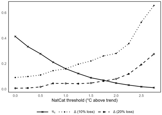
Figure 6. Impact of the NatCat threshold on the NatCat probability ${\pi }_c$ and the difference in loss probabilities ${\pi }_h-{\pi }_l$.

Figure 7 illustrates the impact of the NatCat event threshold on a farmer’s expected utility under index insurance $\mathbb{E}\left(U_I\right)$, for a 10% loss threshold and different loadings ${\lambda }_I$. For low NatCat thresholds (0 to 1.5 °C), there is no demand for insurance with loading factors. When the NatCat threshold is between 0 and about 0.5 °C, there is no demand for index insurance, even when it is offered at the pure premium. This occurs when index insurance does not effectively classify the NatCat, leading to basis risk. For a low loading factor (${\lambda }_I=0.02$), the expected utility reaches its maximum at a NatCat threshold of approximately 2.7 °C above the trend, which therefore represents the optimal trigger threshold for the index-based insurance. Consistent with our theoretical results, a higher loading not only reduces expected utility but also shifts its maximum to a higher NatCat threshold. For ${\lambda }_I=0.06$, insurance demand would only be positive (i.e., expected utility exceeds its minimum) for NatCat thresholds roughly between 2.3 and 3.4 °C. At higher loadings, there is no insurance demand, regardless of the NatCat threshold. Consequently, index insurance demand would occur only if the loading applied to the actuarially fair premium is significantly lower than the range currently observed in the United States (0.2–0.3).

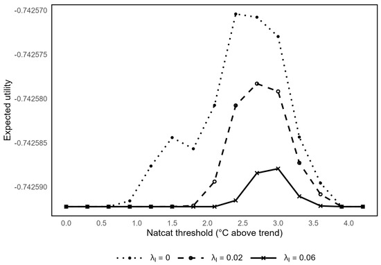
Figure 7. Impact of NatCat definition on index-based insurance $\mathbb{E}\left(U_I\right)$ for a 10% loss threshold with different loadings.

4.3. Insurance Selection

As shown above, with a 10% loss threshold, the maximum loading that allows a positive demand for loss-based insurance is approximately 0.14. With a 20% loss threshold, the maximum loading increases to 0.23. Therefore, if ${\lambda }_L=0.40$, there would be no demand for loss-based insurance. For higher loss thresholds, which correspond to lower probabilities of loss but more severe losses, loss-based insurance becomes more attractive, and farmers are willing to pay higher maximum loadings. In contrast, for index-based insurance, the relationship is reversed (Clarke 2016; Hott and Regner 2023). With a 10% loss threshold, there is positive demand for index insurance up to a ${\lambda }_I$ slightly above 0.114. For a 20% loss threshold, the maximum ${\lambda }_I$ decreases to around 0.056, and for a 25% threshold, it falls further to 0.034.

Figure 8 illustrates the effect of loss definition on demand for index insurance (${\theta }_I$) and loss-based insurance (${\theta }_L$), as well as on the difference in expected utility between them, $\mathbb{E}\left(U_I\right)-\mathbb{E}\left(U_L\right)$. To ensure positive insurance demand, we assume relatively low loadings (${\lambda }_I=0.02$, ${\lambda }_L=0.2$), under which farmers have a greater incentive to purchase insurance (Clarke 2016; Jensen and Barrett 2017). If losses are defined as zero negative deviations from yield trends (i.e., a 0% loss deviation threshold), neither index-based nor loss-based insurance generates positive demand. At a loss threshold of around 2%, the demand for index insurance becomes positive, reaching a maximum of approximately 10%. When the loss threshold exceeds 20%, demand for index insurance falls to zero. Demand for loss-based insurance becomes positive at thresholds around 16% and continues to increase with higher thresholds, reaching a maximum of 35%. Consistent with these results, index insurance is more attractive ($\mathbb{E}\left(U_I\right)>\mathbb{E}\left(U_L\right)$) for low loss thresholds (between 2% and 18%), whereas loss-based insurance is preferable ($\mathbb{E}\left(U_I\right)<\mathbb{E}\left(U_L\right)$) for higher thresholds (above 18%). In other words, index-based insurance is better suited to frequent but small losses, while loss-based insurance is preferable for rare but severe losses that require an accurate assessment of actual damage. This is consistent with the discussion in Clarke (2016) on how basis risk varies with loss size, and with the evidence from (Jensen and Barrett 2017; Miranda and Farrin 2012) that indemnity insurance offers superior protection against catastrophic events.

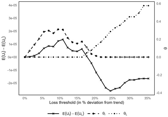
Figure 8. Impact of the loss threshold on insurance demand ${\theta }_{L,I}$ and the difference in expected utility $\mathbb{E}\left(U_I\right)-\mathbb{E}\left(U_L\right)$.

For loss thresholds between 16% and 22%, there is potential demand for both index-based and loss-based insurance. Within this range, simultaneous purchase of both products may be optimal. According to Proposition 2, when both types of insurance are available, demand for index-based insurance is positive only if ${\lambda }_I<{\lambda }_L$ and the two insurance types act as substitutes. This implies that when the loss threshold is slightly above 13%, demand exists only for loss-based insurance. In contrast, when the threshold is slightly below 22%, demand is limited to index-based insurance. For intermediate loss thresholds (i.e., between 16% and 22%), however, joint purchase may be optimal. The combination of index and loss-based insurance can be implemented through a layered contract structure, where the two products act as partial substitutes and complements: index insurance covers mid-range losses, and indemnity insurance protects against catastrophic losses (Barnett et al. 2005; Carter et al. 2016).

Figure 9 illustrates the relationship between insurance demand and the level of risk aversion, as well as the difference in expected utility between the two insurance types. For a given adverse event, a more risk-averse farmer consistently spends more on loss-based insurance, whereas this pattern does not necessarily hold for index-based insurance. This aligns with Clarke (2016), who suggests that the relatively low demand for index-based insurance arises from an infinitely risk-averse individual. For a loss threshold of 10% combined with a NatCat threshold of 2.7 °C, index-based insurance is preferred only by less risk-averse farmers ($\mathbb{E}\left(U_I\right)>\mathbb{E}\left(U_L\right)$). When the loss threshold increases to 20%, index-based insurance ceases to be attractive for any level of risk aversion ($\mathbb{E}\left(U_I\right)<\mathbb{E}\left(U_L\right)$). These results are consistent with earlier findings, indicating that index-based insurance is preferable only for relatively small, more frequent losses.

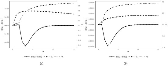
Figure 9. Impact of risk-aversion level on insurance demand ${\theta }_{L,I}$ and the difference in expected utility $\mathbb{E}\left(U_I\right)-\mathbb{E}\left(U_L\right)$ with 2.7 °C NatCat threshold and a (a) 10% loss deviation and (b) 20% loss deviation.

5. Conclusions

Weather-related risks remain a major source of income volatility for farmers but are particularly challenging to insure. Even in countries with mature insurance markets, meaningful coverage for these risks is limited without public intervention. This paper assessed the relative performance of index-based and loss-based insurance for French crop farmers using a combined theoretical and empirical framework.

In this study, we establish the conditions under which traditional insurance, index insurance, or a combination of the two is the preferred choice for the farmer. Our theoretical model shows that farmers’ preferences for index versus loss-based insurance depend not only on premium loadings but also on the market interest rate, the risk-aversion coefficient, the probability of a NatCat event, and the difference in loss probability with and without a NatCat event. The model shows that full insurance occurs only under specific conditions, including a zero market interest rate. Under high market loadings, demand for both index and loss-based insurance remains essentially zero. This finding underscores a key policy implication: without lower loadings or targeted public support, weather-related agricultural risks are unlikely to be insured at a meaningful scale.

Empirically, we identified mean spring temperature as the weather variable most strongly associated with winter barley yield losses, making it the most promising basis for an index. Simulations show that positive demand for index-based insurance arises only when its loading is substantially lower than that of the loss-based insurance, largely due to basis risk. For a certain level of risk aversion, index-based insurance is most attractive for frequent, low-severity losses, while traditional loss-based insurance outperforms it for rare, high-severity losses that farmers are willing to pay higher premiums. Increasing risk aversion raises the demand for traditional loss-based insurance, but not necessarily for index-based insurance. Overall, highly risk-averse farmers consistently prefer traditional insurance over index-based insurance.

Nonetheless, this study has some limitations. First, the model does not allow farmers to diversify production risk across crops or regions, which may overstate the insurance’s attractiveness relative to real-world conditions. Second, losses are modeled as a binary variable. Although this assumption simplifies the analysis, it does not fully reflect the continuous nature of agricultural yield losses. Third, under the assumption of heterogeneous wealth among farmers, the CARA utility function is no longer appropriate. Nevertheless, its analytical tractability has allowed us to derive closed-form solutions for the optimal strategies. Importantly, the risk aversion coefficient is simply set in advance without surveying or estimating, so the results may not accurately reflect an individual’s risk profile. Lastly, relatively low loadings factor on index-based insurance may lead to irrationality. Despite these limitations, the simplified framework delivers relevant insights into the potential role of index and loss-based insurance for French crop farmers. Future research should also incorporate additional factors, such as multi-crop and multi-region settings, differences between developed and developing countries, and behavioral aspects. While the assumptions of binary losses and a CARA utility function simplify the analysis, they do not fully capture real-world conditions.

Appendix A.1. Proof of Proposition 1

Appendix A.1.1. Traditional Loss-Based Insurance

The optimal savings amount $s_L^{*}$ and coverage rate ${\theta }_L^{*}$ are the solution to the following inequality-constrained optimization problem:

$$\underset{s_L,{\theta }_L}{max}\mathbb{E}\left[U_L(s_L,{\theta }_L)\right]\hspace{1em}\mathrm{subject} \mathrm{to} \mathrm{the} \mathrm{constraints}\hspace{1em}\left\{\begin{array}{c}0\le {\theta }_L\le 1\hfill \\ (1+{\lambda }_L)\pi l{\theta }_L+s_L\le 1.\hfill \end{array}\right.$$

(A1)

Step 1: We first prove that the Hessian matrix $\left(\begin{array}{cc}{u}_{L,ss}& u_{L,s\theta }\\ u_{L,\theta s}& u_{L,\theta \theta }\end{array}\right)$ is negative definite, where $u_{L,ij}={\partial }_i{\partial }_j\mathbb{E}\left[U_L(s_L,{\theta }_L)\right]:$

$$\begin{array}{cc}\hfill u_{L,ss}& =-\alpha e^{-\alpha \left[1-s_L-(1+{\lambda }_L)\pi l{\theta }_L\right]}-\alpha \pi (1+r)e^{-\alpha \left(1+s_L(1+r)-l+l{\theta }_L\right)}-\alpha (1-\pi )(1+r)e^{-\alpha \left(1+s_L(1+r)\right)},\hfill \\ \hfill u_{L,\theta \theta }& =-\alpha {(1+{\lambda }_L)}^2{\pi }^2{l}^2{e}^{-\alpha \left[1-s_L-(1+{\lambda }_L)\pi l{\theta }_L\right]}-{\displaystyle \frac{\alpha \pi l^2}{1+r}}{e}^{-\alpha \left(1+s_L(1+r)-l+l{\theta }_L\right)},\hfill \\ \hfill u_{L,s\theta }& =u_{L,\theta s}=-\alpha (1+{\lambda }_L)\pi l{e}^{-\alpha \left[1-s_L-(1+{\lambda }_L)\pi l{\theta }_L\right]}-\alpha \pi l{e}^{-\alpha \left(1+s_L(1+r)-l+l{\theta }_L\right)}.\hfill \end{array}$$

Recall that a symmetric matrix is negative definite if and only if all of its principal minors of even order are positive and all of its principal minors of odd order are negative. Thus, we have to prove that $u_{L,ss}<0$ and $u_{L,ss}{u}_{L,\theta \theta }-u_{L,s\theta }^2>0$.

Since $u_{L,ss},u_{L,\theta \theta }<0$ and

$$\begin{array}{c}{u}_{L,ss}{u}_{L,\theta \theta }-u_{L,s\theta }^2={\displaystyle \frac{{\alpha }^2{l}^2\pi }{1+r}}{[1-(1+{\lambda }_L)(1+r)\pi ]}^2{e}^{-\alpha \left[2+s_{L}r-l+(1-(1+{\lambda }_L)\pi )l{\theta }_L\right]}\hfill \\ +{\alpha }^2{l}^2(1+r)\pi (1-\pi )\left[{(1+{\lambda }_L)}^2\pi e^{-\alpha \left[2+s_{L}r-(1+{\lambda }_L)\pi l{\theta }_L\right]}+{\displaystyle \frac{e^{-\alpha \left(2+2s_L(1+r)-l+l{\theta }_L\right)}}{1+r}}\right]>0,\hfill \end{array}$$

then the Hessian matrix is negative definite, and the maximization problem has a unique interior maximum.

Step 2: The optimal amounts $s_L^{*}$ and ${\theta }_L^{*}$ satisfy the Karush–Kuhn–Tucker (KKT) conditions, i.e., there exist ${\mu }_i\in {\mathbb{R}}_{-}$, $i=1,2,3$ such that:

$$\left\{\begin{array}{c}\nabla \mathbb{E}\left[U_L(s,\theta )\right]+{\sum }_{i=1}^3{\mu }_i\nabla g_i(s,\theta )=0,\hfill \\ {\mu }_i{g}_i(s,\theta )=0\forall i\in \{1,2,3\},\hfill \end{array}\right.$$

(A2)

where $g_1(s,\theta )=-\theta$, $g_2(s,\theta )=\theta -1$, $g_3(s,\theta )=(1+{\lambda }_L)\pi l\theta +s-1.$

Let note $A_L=\{(s,\theta )\in {\mathbb{R}}^2:g_i(s,\theta )\le 0\forall i=1,2,3\}$ the feasible region and $I=\{i:g_i\left(x\right)=0\}$, for $x\in A_L$ the set of active (linear) constraints. Note that $g_1$ and $g_2$ cannot both be equal to zero at the same time. Therefore the possibles cases are: $I=\{1,3\}$, $I=\{2,3\}$, $I=\left\{1\right\}$, $I=\left\{2\right\}$, $I=\left\{3\right\}$ and $I=\{\varnothing \}$.

• $I=\{1,3\}$: Hence $s=1$ and $\theta =0$, and the KKT conditions (A2) are:

  $$\left\{\begin{array}{c}-1+\pi e^{-\alpha \left(2+r-l\right)}+(1-\pi )e^{-\alpha (2+r)}+{\mu }_3=0\hfill \\ -(1+{\lambda }_L)\pi l+{\displaystyle \frac{l\pi }{1+r}}{e}^{-\alpha \left(2+r-l\right)}-{\mu }_1+{\mu }_3(1+{\lambda }_L)\pi l=0\hfill \\ {\mu }_1,{\mu }_3\in {\mathbb{R}}_{-}.\hfill \end{array}\right.$$

  The first condition implies ${\mu }_3=1-\pi e^{-\alpha \left(2+r-l\right)}-(1-\pi )e^{-\alpha (2+r)}$.

Since $1-\pi e^{-\alpha \left(2+r-l\right)}-(1-\pi )e^{-\alpha (2+r)}=e^{-\alpha (2+r)}(e^{\alpha l}-1)\left[{\displaystyle \frac{e^{\alpha (2+r)}-1}{e^{\alpha l}-1}}-\pi \right]>0$, then $(1,0)$ is not a KKT point.

Similar reasoning is used for $I=\{2,3\}$ and $I=\left\{3\right\}$ to prove that there is no solution to the KKT system.

• $I=\left\{1\right\}$: Hence $\theta =0$ and the KKT conditions (A2) are:

  $$\left\{\begin{array}{c}-e^{\alpha s_L}+\pi e^{-\alpha \left(s_L(1+r)-l\right)}+(1-\pi )e^{-\alpha s_L(1+r)}=0\hfill \\ -(1+{\lambda }_L)\pi l{e}^{-\alpha (1-s_L)}+{\displaystyle \frac{l\pi }{1+r}}{e}^{-\alpha \left(1+s_L(1+r)-l\right)}-{\mu }_1=0\hfill \\ {\mu }_1\in {\mathbb{R}}_{-}.\hfill \end{array}\right.$$

  So $s={\displaystyle \frac{ln\left(1-\pi +\pi e^{\alpha l}\right)}{\alpha (2+r)}}$ and ${\mu }_1={\displaystyle \frac{l\pi e^{-\alpha }{\left(1-\pi +\pi e^{\alpha l}\right)}^{\frac{1}{2+r}}}{1+r}}\left[-(1+{\lambda }_L)(1+r)+{\displaystyle \frac{e^{\alpha l}}{1-\pi +\pi e^{\alpha l}}}\right].$ Therefore $\left({\displaystyle \frac{ln\left(1-\pi +\pi e^{\alpha l}\right)}{\alpha (2+r)}},0\right)$ is a feasible point satisfying KKT conditions if $1+{\lambda }_L\ge b_L\left(\alpha \right)$.
• $I=\left\{2\right\}$: Hence $\theta =1$ and KKT conditions (A2) are:

  $$\left\{\begin{array}{c}-e^{-\alpha \left[1-s_L-(1+{\lambda }_L)\pi l\right]}+\pi e^{-\alpha \left(1+s_L(1+r)\right)}+(1-\pi )e^{-\alpha \left(1+s_L(1+r)\right)}=0\hfill \\ -(1+{\lambda }_L)\pi l{e}^{-\alpha \left[1-s_L-(1+{\lambda }_L)\pi l\right]}+{\displaystyle \frac{\pi l}{1+r}}{e}^{-\alpha \left(1+s_L(1+r)\right)}+{\mu }_2=0\hfill \\ {\mu }_3\in {\mathbb{R}}_{-}.\hfill \end{array}\right.$$

  Since $s=-{\displaystyle \frac{(1+{\lambda }_L)\pi l}{2+r}}$ and ${\mu }_2={\displaystyle \frac{(r+{\lambda }_L+r{\lambda }_L)\pi l}{1+r}}{e}^{-\alpha +{\displaystyle \frac{\alpha (1+{\lambda }_L)(1+r)\pi l}{2+r}}}\ge 0$, then $\left(-{\displaystyle \frac{(1+{\lambda }_L)\pi l}{2+r}},1\right)$ is a feasible point only if $r={\lambda }_L=0$.
• $I=\{\varnothing \}$: In this case KKT conditions (A2) are:

  $$\left\{\begin{array}{c}-e^{\alpha \left[s_L+(1+{\lambda }_L)\pi l{\theta }_L\right]}+\pi e^{-\alpha \left[s_L(1+r)-l+l{\theta }_L\right]}+(1-\pi )e^{-\alpha s_L(1+r)}=0\hfill \\ -(1+{\lambda }_L)e^{\alpha \left[s_L+(1+{\lambda }_L)\pi l{\theta }_L\right]}+{\displaystyle \frac{1}{1+r}}{e}^{-\alpha \left[s_L(1+r)-l+l{\theta }_L\right]}=0\hfill \end{array}\right.$$

  If $1+{\lambda }_L\le b_L\left(\alpha \right)$, $(s_L^{*},{\theta }_L^{*})\in A_L$ satisfies KKT conditions, where

  $$\begin{array}{cc}\hfill s_L^{*}& =-{\displaystyle \frac{(1+{\lambda }_L)\pi l}{2+r}}-{\displaystyle \frac{1}{(2+r)\alpha }}ln\left((1+{\lambda }_L)(1+r)\right)+{\displaystyle \frac{1+(1+{\lambda }_L)\pi }{(2+r)\alpha }}ln\left\{{\displaystyle \frac{(1+r)(1+{\lambda }_L)(1-\pi )}{1-(1+r)(1+{\lambda }_L)\pi }}\right\},\hfill \\ \hfill {\theta }_L^{*}& =1-{\displaystyle \frac{1}{\alpha l}}ln\left\{{\displaystyle \frac{(1+r)(1+{\lambda }_L)(1-\pi )}{1-(1+r)(1+{\lambda }_L)\pi }}\right\}.\hfill \end{array}$$

Appendix A.1.2. Index Insurance

The optimal amount of savings $s_I^{*}$ and insurance ${\theta }_I^{*}$ are solutions of the following inequality-constrained optimization problem:

$$\underset{s_I,{\theta }_I}{max}\mathbb{E}\left[U_I(s_I,{\theta }_I)\right]\hspace{1em}\mathrm{subject} \mathrm{to} \mathrm{the} \mathrm{constraints}\hspace{1em}\left\{\begin{array}{c}0\le {\theta }_I\le 1\hfill \\ (1+{\lambda }_I){\pi }_{c}l{\theta }_I+s\le 1.\hfill \end{array}\right.$$

(A3)

Step 1: As before, we easily prove that the Hessian matrix $\left(\begin{array}{cc}{u}_{I,ss}& u_{I,s\theta }\\ u_{I,\theta s}& u_{I,\theta \theta }\end{array}\right)$ is negative definite, where $u_{I,ij}={\partial }_i{\partial }_j\mathbb{E}\left[U_I(s_I,{\theta }_I)\right]:$

$$\begin{array}{cc}\hfill u_{I,ss}=& -\alpha e^{-\alpha \left[1-s_I-(1+{\lambda }_I){\pi }_{c}l{\theta }_I\right]}-\alpha {\pi }_c(1+r)e^{-\alpha \left(1+s_I(1+r)+l{\theta }_I\right)}\left({\pi }_h{e}^{\alpha l}+1-{\pi }_h\right)\hfill \\ \hfill & -\alpha (1-{\pi }_c)(1+r)e^{-\alpha (1+s_I(1+r))}\left({\pi }_l{e}^{\alpha l}+1-{\pi }_l\right)\hfill \\ \hfill u_{I,\theta \theta }=& -\alpha {(1+{\lambda }_I)}^2{\pi }_c^2{l}^2{e}^{-\alpha \left[1-s_I-(1+{\lambda }_I){\pi }_{c}l{\theta }_I\right]}-{\displaystyle \frac{\alpha {\pi }_c{l}^2}{1+r}}{e}^{-\alpha \left(1+s_I(1+r)+l{\theta }_I\right)}\left({\pi }_h{e}^{\alpha l}+1-{\pi }_h\right)\hfill \\ \hfill u_{I,s\theta }=& u_{I,\theta s}=-\alpha (1+{\lambda }_I){\pi }_{c}l{e}^{-\alpha \left[1-s_I-(1+{\lambda }_I){\pi }_{c}l{\theta }_I\right]}-\alpha {\pi }_{c}l{e}^{-\alpha \left(1+s_I(1+r)+l{\theta }_I\right)}\left({\pi }_h{e}^{\alpha l}+1-{\pi }_h\right).\hfill \end{array}$$

Step 2: The optimal amount of savings $s_I^{*}$ and insurance ${\theta }_I^{*}$ satisfy the Karush–Kuhn–Tucker (KKT) conditions, i.e., there exist ${\mu }_i\in {\mathbb{R}}_{-}$, $i=1,2,3$ such that:

$$\left\{\begin{array}{c}\nabla \mathbb{E}\left[U_I(s,\theta )\right]+{\sum }_{i=1}^3{\mu }_i\nabla g_i(s,\theta )=0,\hfill \\ {\mu }_i{g}_i(s,\theta )=0\forall i\in \{1,2,3\},\hfill \end{array}\right.$$

(A4)

where $g_1(s,\theta )=-\theta$, $g_2(s,\theta )=\theta -1$, and $g_3(s,\theta )=(1+{\lambda }_I){\pi }_c{i}_I\theta +s-1.$

As in the case of traditional loss-based insurance, we introduce the feasible region $A_I=\{(s,\theta )\in {\mathbb{R}}^2:g_i(s,\theta )\le 0\forall i=1,2,3\}$ and the set of active (linear) constraints $I=\{i:g_i\left(x\right)=0\}$, for $x\in A_I$. Note that $g_2$ and $g_3$ cannot both be null at the same time. Therefore the same cases as before must be examined: $I=\{1,3\}$, $I=\{2,3\}$, $I=\left\{1\right\}$, $I=\left\{2\right\}$, $I=\left\{3\right\}$ and $I=\{\varnothing \}$. One can prove that there is no solution that verifies (A4) when $I=\{1,2\}$, $I=\{2,3\}$ and $I=\left\{3\right\}$.

• $I=\left\{1\right\}$: Hence $\theta =0$ and the KKT conditions (A4) are:

  $$\left\{\begin{array}{c}-e^{\alpha s_I}+{\pi }_c{e}^{-\alpha s_I(1+r)}({\pi }_h{e}^{\alpha l}+1-{\pi }_h)+(1-{\pi }_c)e^{-\alpha s_I(1+r)}({\pi }_l{e}^{\alpha l}+1-{\pi }_l)=0\hfill \\ -(1+{\lambda }_I){\pi }_{c}l{e}^{-\alpha (1-s_I)}+{\displaystyle \frac{{\pi }_{c}l}{1+r}}{e}^{-\alpha \left[1+s_I(1+r)\right]}({\pi }_h{e}^{\alpha l}+1-{\pi }_h)-{\mu }_1=0\hfill \\ {\mu }_1\in {\mathbb{R}}_{-}.\hfill \end{array}\right.$$

  We easily find $s={\displaystyle \frac{ln\left(1-\pi +\pi e^{\alpha l}\right)}{\alpha (2+r)}}$ and ${\mu }_1={\displaystyle \frac{l{\pi }_c{e}^{-\alpha }{\left(1-\pi +\pi e^{\alpha l}\right)}^{\frac{1}{2+r}}}{1+r}}\left[-(1+{\lambda }_L)(1+r)+{\displaystyle \frac{1-{\pi }_h+{\pi }_h{e}^{\alpha l}}{1-\pi +\pi e^{\alpha l}}}\right].$ So $\left({\displaystyle \frac{ln\left(1-\pi +\pi e^{\alpha l}\right)}{\alpha (2+r)}},0\right)$ is a feasible point satisfying (A4) if $1+{\lambda }_I\ge b_I\left(\alpha \right)$. Let’s note that ${\displaystyle \frac{1-{\pi }_h+{\pi }_h{e}^{\alpha l}}{1-\pi +\pi e^{\alpha l}}}<1⟺{\pi }_l>{\pi }_h$. Therefore if ${\pi }_l>{\pi }_h$, then $\left({\displaystyle \frac{ln\left(1-\pi +\pi e^{\alpha l}\right)}{\alpha (2+r)}},0\right)$ is solution of (A4) with no additional conditions.
• $I=\left\{2\right\}$: Hence $\theta =1$ and the KKT conditions are:

  $$\left\{\begin{array}{c}-e^{\alpha \left[s_I+(1+{\lambda }_I){\pi }_{c}l\right]}+{\pi }_c{e}^{-\alpha \left[s_I(1+r)+l\right]}({\pi }_h{e}^{\alpha l}+1-{\pi }_h)+(1-{\pi }_c)e^{-\alpha s_I(1+r)}({\pi }_l{e}^{\alpha l}+1-{\pi }_l)=0\hfill \\ -(1+{\lambda }_I){\pi }_{c}l{e}^{-\alpha \left[1-s_I+(1+{\lambda }_I){\pi }_{c}l\right]}+{\displaystyle \frac{{\pi }_{c}l}{1+r}}{e}^{-\alpha \left[1+s_I(1+r)+i_I{\theta }_I\right]}({\pi }_h{e}^{\alpha l}+1-{\pi }_h)+{\mu }_2=0\hfill \\ {\mu }_2\in {\mathbb{R}}_{-}.\hfill \end{array}\right.$$

  We find that $e^{-\alpha s_I^{*}(2+r)}={\displaystyle \frac{e^{\alpha (1+{\lambda }_I){\pi }_{c}l}}{{\pi }_c{e}^{-\alpha l}({\pi }_h{e}^{\alpha l}+1-{\pi }_h)+(1-{\pi }_c)({\pi }_l^{\alpha l}+1-{\pi }_l)}}$. Since ${\mu }_2\in {\mathbb{R}}_{-}$, then $(1+{\lambda }_I)(1+r)\le {\displaystyle \frac{e^{-\alpha l}({\pi }_h{e}^{\alpha l}+1-{\pi }_h)}{{\pi }_c{e}^{-\alpha l}({\pi }_h{e}^{\alpha l}+1-{\pi }_h)+(1-{\pi }_c)({\pi }_l^{\alpha l}+1-{\pi }_l)}}\le 1$, where ${\displaystyle \frac{e^{-\alpha l}({\pi }_h{e}^{\alpha l}+1-{\pi }_h)}{{\pi }_c{e}^{-\alpha l}({\pi }_h{e}^{\alpha l}+1-{\pi }_h)+(1-{\pi }_c)({\pi }_l^{\alpha l}+1-{\pi }_l)}}=1$ when ${\pi }_h=1$ and ${\pi }_l=0$. Therefore ${\theta }_I^{*}=1$ only if ${\pi }_h=1$, ${\pi }_l=0$, $r={\lambda }_I=0$.
• $I=\{\varnothing \}$: In this case KKT system is:

  $$\left\{\begin{array}{c}-e^{\alpha \left[s_I+(1+{\lambda }_I){\pi }_{c}l{\theta }_I\right]}+{\pi }_c{e}^{-\alpha \left[s_I(1+r)+l{\theta }_I\right]}({\pi }_h{e}^{\alpha l}+1-{\pi }_h)+(1-{\pi }_c)e^{-\alpha s_I(1+r)}({\pi }_l{e}^{\alpha l}+1-{\pi }_l)=0\hfill \\ -(1+{\lambda }_I)e^{\alpha \left[s_I+(1+{\lambda }_I){\pi }_{c}l{\theta }_I\right]}+{\displaystyle \frac{1}{1+r}}{e}^{-\alpha \left[s_I(1+r)+l{\theta }_I\right]}({\pi }_h{e}^{\alpha l}+1-{\pi }_h)=0\hfill \end{array}\right.$$

  If $1+{\lambda }_I\le b_I\left(\alpha \right)$, then $(s_I^{*},{\theta }_I^{*})\in A_I$ satisfies KKT conditions, where

  $$\begin{array}{cc}\hfill s_I^{*}=& {\displaystyle \frac{1}{\alpha (2+r)}}ln\left\{{\displaystyle \frac{(1-{\pi }_c)({\pi }_l{e}^{\alpha l}+1-{\pi }_l)}{1-(1+{\lambda }_I)(1+r){\pi }_c}}\right\}\hfill \\ \hfill & +{\displaystyle \frac{(1+{\lambda }_I){\pi }_c}{\alpha (2+r)}}ln\left\{{\displaystyle \frac{(1+r)(1+{\lambda }_I)(1-{\pi }_c)({\pi }_l{e}^{\alpha l}+1-{\pi }_l)}{[1-(1+{\lambda }_I)(1+r){\pi }_c]({\pi }_h{e}^{\alpha l}+1-{\pi }_h)}}\right\}\hfill \\ \hfill {\theta }_I^{*}=& {\displaystyle \frac{1}{\alpha l}}ln\left\{{\displaystyle \frac{[1-(1+r)(1+{\lambda }_I){\pi }_c]({\pi }_h{e}^{\alpha l}+1-{\pi }_h)}{(1+r)(1+{\lambda }_I)(1-{\pi }_c)({\pi }_l{e}^{\alpha l}+1-{\pi }_l)}}\right\}\hfill \end{array}$$

Appendix A.2. Proof of Proposition 2

The approach is the same as in the proof of Proposition 1.

Step 1: We first prove that the Hessian matrix $\left(\begin{array}{ccc}{u}_{ss}& u_{s{\theta }_I}& u_{s{\theta }_L}\\ u_{s{\theta }_I}& u_{{\theta }_I{\theta }_I}& u_{{\theta }_I{\theta }_L}\\ u_{s{\theta }_L}& u_{{\theta }_I{\theta }_L}& u_{{\theta }_L{\theta }_L}\end{array}\right)$ is negative definite, where $u_{ij}={\partial }_i{\partial }_j\mathbb{E}\left[U_I(s,{\theta }_I,{\theta }_L)\right]$:

$$\begin{array}{cc}\hfill u_{ss}& =-\alpha A-\alpha {\pi }_c(1+r)B{e}^{-\alpha l{\theta }_I}\left[{\pi }_h{e}^{\alpha l-\alpha l{\theta }_L}+1-{\pi }_h\right]-\alpha (1-{\pi }_c)(1+r)B\left[{\pi }_l{e}^{\alpha l-\alpha l{\theta }_L}+1-{\pi }_l\right]\hfill \\ \hfill u_{{\theta }_I{\theta }_I}& =-\alpha {(1+{\lambda }_I)}^2{\pi }_c^2{l}^{2}A-{\displaystyle \frac{\alpha {\pi }_c}{1+r}}{l}^{2}B{e}^{-\alpha l{\theta }_I}\left[{\pi }_h{e}^{\alpha l-\alpha l{\theta }_L}+1-{\pi }_h\right]\hfill \\ \hfill u_{{\theta }_L{\theta }_L}& =-\alpha {(1+{\lambda }_L)}^2{\pi }^2{l}^{2}A-{\displaystyle \frac{\alpha }{1+r}}{l}^{2}B{e}^{\alpha l-\alpha l{\theta }_L}\left[{\pi }_c{\pi }_h{e}^{-\alpha l{\theta }_I}+(1-{\pi }_c){\pi }_l\right]\hfill \\ \hfill u_{s{\theta }_I}& =-\alpha (1+{\lambda }_I){\pi }_{c}lA-\alpha {\pi }_{c}l{e}^{-\alpha l{\theta }_I}B\left[{\pi }_h{e}^{\alpha l-\alpha l{\theta }_L}+1-{\pi }_h\right]\hfill \\ \hfill u_{s{\theta }_L}& =-\alpha (1+{\lambda }_L)\pi lA-\alpha lB{e}^{\alpha l-\alpha l{\theta }_L}\left[{\pi }_c{\pi }_h{e}^{-\alpha l{\theta }_I}+(1-{\pi }_c){\pi }_l\right]\hfill \\ \hfill u_{{\theta }_I{\theta }_L}& =-\alpha (1+{\lambda }_I)(1+{\lambda }_L)\pi {\pi }_c{l}^{2}A-{\displaystyle \frac{\alpha {\pi }_c{\pi }_h}{1+r}}{l}^{2}B{e}^{-\alpha (-l+l{\theta }_L+l{\theta }_I)}\hfill \\ \hfill A& =e^{-\alpha \left[1-s-(1+{\lambda }_L)\pi l{\theta }_L-(1+{\lambda }_I){\pi }_{c}l{\theta }_I\right]},B=e^{-\alpha [1+s(1+r\left)\right]}.\hfill \end{array}$$

The Hessian matrix is negative definite if its principal minors of orders 1 and 3 are negative and the principal minor of order 2 is positive, i.e., $u_{ss}<0$ (obvious), $u_{ss}{u}_{{\theta }_I{\theta }_I}-u_{s{\theta }_I}^2>0$ and $\left|\begin{array}{ccc}{u}_{ss}& u_{s{\theta }_I}& u_{s{\theta }_L}\\ u_{s{\theta }_I}& u_{{\theta }_I{\theta }_I}& u_{{\theta }_I{\theta }_L}\\ u_{s{\theta }_L}& u_{{\theta }_I{\theta }_L}& u_{{\theta }_L{\theta }_L}\end{array}\right|<0.$ After some calculations, these inequalities are verified.

Step 2: The optimal amount of savings $s^{*}$ and insurances ${\theta }_I^{*},{\theta }_L^{*}$ satisfy the Karush–Kuhn–Tucker (KKT) conditions, i.e., there exist ${\mu }_i\in {\mathbb{R}}_{-}$, $i=1,\dots ,4$ such that:

$$\left\{\begin{array}{c}\nabla \mathbb{E}\left[U(s,{\theta }_L,{\theta }_I)\right]+{\sum }_{i=1}^4{\mu }_i\nabla g_i(s,\theta )=0,\hfill \\ {\mu }_i{g}_i(s,\theta )=0\forall i\in \{1,2,3,4\},\hfill \end{array}\right.$$

(A5)

where $g_1(s,{\theta }_L,{\theta }_I)=-{\theta }_L$, $g_2(s,{\theta }_L,{\theta }_I)=-{\theta }_I$, $g_3(s,{\theta }_L,{\theta }_I)={\theta }_L+{\theta }_I-1$, and $g_4(s,{\theta }_L,{\theta }_I)=(1+{\lambda }_L)\pi l{\theta }_L+(1+{\lambda }_I){\pi }_{c}l{\theta }_I+s-1.$

As in the previous cases, we introduce the feasible region $A_{L,I}=\{(s,{\theta }_L,{\theta }_I)\in {\mathbb{R}}^3:g_i(s,\theta )\le 0\forall i=1,\dots ,4\}$ and the set of active (linear) constraints $I=\{i:g_i\left(x\right)=0\}$, for $x\in A_{L,I}$. Note that if $g_1$ and $g_2$ are null, then $g_3\ne 0$.

Appendix A.2.1. No Insurance Policy

The farmer does not insure their crop when ${\theta }_L={\theta }_I=0$, which corresponds to $g_1(s,{\theta }_L,{\theta }_I)=g_2(s,{\theta }_L,{\theta }_I)=0$. We easily prove that if $I=\{1,2,4\}$, the system (A5) has no solution. When $I=\{1,2\}$, the KKT conditions are:

$$\left\{\begin{array}{c}-e^{\alpha s}+e^{-\alpha s(1+r)}(\pi e^{\alpha l}+1-\pi )=0\hfill \\ -(1+{\lambda }_L)\pi l{e}^{-\alpha (1-s)}+{\displaystyle \frac{l\pi }{1+r}}{e}^{-\alpha \left(1+s(1+r)-l\right)}-{\mu }_1=0\hfill \\ -(1+{\lambda }_I){\pi }_{c}l{e}^{-\alpha (1-s)}+{\displaystyle \frac{{\pi }_{c}l}{1+r}}{e}^{-\alpha \left[1+s(1+r)\right]}({\pi }_h{e}^{\alpha l}+1-{\pi }_h)-{\mu }_2=0\hfill \\ {\mu }_1,{\mu }_2\in {\mathbb{R}}_{-}.\hfill \end{array}\right.$$

We find $s={\displaystyle \frac{ln\left(1-\pi +\pi e^{\alpha l}\right)}{\alpha (2+r)}}$, ${\mu }_2={\displaystyle \frac{l\pi e^{-\alpha }{\left(1-\pi +\pi e^{\alpha l}\right)}^{\frac{1}{2+r}}}{1+r}}\left[-(1+{\lambda }_L)(1+r)+{\displaystyle \frac{e^{\alpha l}}{1-\pi +\pi e^{\alpha l}}}\right]$ and ${\mu }_3={\displaystyle \frac{l{\pi }_c{e}^{-\alpha }{\left(1-\pi +\pi e^{\alpha l}\right)}^{\frac{1}{2+r}}}{1+r}}\left[-(1+{\lambda }_I)(1+r)+{\displaystyle \frac{1-{\pi }_h+{\pi }_h{e}^{\alpha l}}{1-\pi +\pi e^{\alpha l}}}\right].$ So $\left({\displaystyle \frac{ln\left(1-\pi +\pi e^{\alpha l}\right)}{\alpha (2+r)}},0,0\right)$ is a feasible point if $1+{\lambda }_L\ge b_L\left(\alpha \right)$ and $1+{\lambda }_I\ge b_I\left(\alpha \right)$.

Appendix A.2.2. Only Traditional Insurance Policy

The farmer chooses only traditional insurance when ${\theta }_I=0$ (so $g_2(s,{\theta }_L,{\theta }_I)=0$) and ${\theta }_L>0$ (so $g_1(s,{\theta }_L,{\theta }_I)<0$). We easily prove that there is no solution to (A5) when $I=\{2,3\}$, $I=\{2,4\}$ and $I=\{2,3,4\}$. When $I=\left\{2\right\}$, the KKT conditions are:

$$\left\{\begin{array}{c}-e^{\alpha \left[s+(1+{\lambda }_L)\pi l{\theta }_L\right]}+e^{-\alpha s(1+r)}\left(\pi e^{\alpha (l-{\theta }_L)}+1-\pi \right)=0\hfill \\ -(1+{\lambda }_L)e^{\alpha \left[s+(1+{\lambda }_L)\pi l{\theta }_L\right]}+{\displaystyle \frac{1}{1+r}}{e}^{-\alpha \left[s(1+r)-l+l{\theta }_L\right]}=0\hfill \\ -(1+{\lambda }_I){\pi }_{c}l{e}^{\alpha \left[s+(1+{\lambda }_L)\pi l{\theta }_L\right]}+{\displaystyle \frac{{\pi }_{c}l}{1+r}}{e}^{-\alpha s(1+r)}\left[{\pi }_h{e}^{\alpha l(1-{\theta }_L)}+1-{\pi }_h\right]-{\mu }_2=0\hfill \\ {\mu }_2\in {\mathbb{R}}_{-}.\hfill \end{array}\right.$$

The first two equalities give $s^{*}=s_L^{*}$ and ${\theta }_L^{*}$ are the optimal savings and insurance in Proposition 1 (1b) provided that $1+{\lambda }_L\le b_L\left(\alpha \right)$. Therefore $\left(s^{*},{\theta }_L^{*},0\right)$ is a KKT point if $1+{\lambda }_L\le b_L\left(\alpha \right)$ and

$$-(1+{\lambda }_I)e^{\alpha \left[s^{*}+(1+{\lambda }_L)\pi l{\theta }_L^{*}\right]}+{\displaystyle \frac{1}{1+r}}{e}^{-\alpha s^{*}(1+r)}\left[{\pi }_h{e}^{\alpha l(1-{\theta }_L^{*})}+1-{\pi }_h\right]\le 0.$$

The last condition implies that $(1+{\lambda }_I)(1+r)\ge (1+{\lambda }_L)(1+r){\displaystyle \frac{{\pi }_h-\pi }{1-\pi }}+{\displaystyle \frac{1-{\pi }_h}{1-\pi }}.$ So this conditions is verified when $(1+{\lambda }_I)(1+r)\ge {\displaystyle \underset{x}{max}}{\displaystyle \frac{{\pi }_h-\pi }{1-\pi }}x+{\displaystyle \frac{1-{\pi }_h}{1-\pi }}$ for $x\in \left[1;{\displaystyle \frac{e^{\alpha l}}{1-\pi +\pi e^{\alpha l}}}\right]$. The function $f\left(x\right)={\displaystyle \frac{{\pi }_h-\pi }{1-\pi }}x+{\displaystyle \frac{1-{\pi }_h}{1-\pi }}$ is increasing if ${\pi }_h>\pi$ ($⟺{\pi }_h>{\pi }_l$) and decreasing if ${\pi }_h\le {\pi }_l$. Moreover $f\left(1\right)=1$ and $f\left({\displaystyle \frac{e^{\alpha l}}{1-\pi +\pi e^{\alpha l}}}\right)={\displaystyle \frac{{\pi }_h{e}^{\alpha l}+1-{\pi }_h}{1-\pi +\pi e^{\alpha l}}}.$ We conclude by noting that ${\displaystyle \frac{{\pi }_h{e}^{\alpha l}+1-{\pi }_h}{1-\pi +\pi e^{\alpha l}}}\le 1$ if ${\pi }_h\le {\pi }_l$ and in this case the inequality satisfied by $(1+{\lambda }_I)(1+r)$ is always true.

Appendix A.2.3. Only Index Insurance Policy

The farmer chooses only index insurance when ${\theta }_L=0$ (so $g_1(s,{\theta }_L,{\theta }_I)=0$) and ${\theta }_I>0$ (so $g_2(s,{\theta }_L,{\theta }_I)<0$). We will not detail the calculations, but the reasoning is similar that used previously in the case of traditional insurance.

Appendix A.2.4. Two Different Insurance Policies

The farmer chooses both insurances when ${\theta }_I,{\theta }_L>0$ (so $g_2(s,{\theta }_L,{\theta }_I),g_1(s,{\theta }_L,{\theta }_I)<0$). We will only detail the case $I=\{\varnothing \}$. The KKT conditions (A4) can be written as:

$$\left\{\begin{array}{c}A={\pi }_{c}B{e}^{-\alpha l{\theta }_I}\left[{\pi }_h{e}^{\alpha l(1-{\theta }_L)}+1-{\pi }_h\right]+(1-{\pi }_c)B\left[{\pi }_l{e}^{\alpha l(1-{\theta }_L)}+1-{\pi }_l\right]\hfill \\ (1+{\lambda }_L)A={\displaystyle \frac{1}{1+r}}B{e}^{\alpha l(1-{\theta }_L)}\left[{\displaystyle \frac{{\pi }_c{\pi }_h}{\pi }}{e}^{-\alpha l{\theta }_I}+{\displaystyle \frac{(1-{\pi }_c){\pi }_l}{\pi }}\right]\hfill \\ (1+{\lambda }_I)A={\displaystyle \frac{1}{1+r}}B{e}^{-\alpha l{\theta }_I}[{\pi }_h{e}^{\alpha l(1-{\theta }_L)}+1-{\pi }_h],\hfill \end{array}\right.$$

where A and B are the notations used above.

We apply the same reasoning as Hott and Regner (2023) and we find the following some necessary conditions for the existence of a solution.

Remark A1.

1. 

Since ${\displaystyle \frac{{\pi }_c{\pi }_h}{\pi }}+{\displaystyle \frac{(1-{\pi }_c){\pi }_l}{\pi }}=1$, then $(1+{\lambda }_L)A$ is a convex combination of ${\displaystyle \frac{B{e}^{\alpha l(1-{\theta }_L-{\theta }_I)}}{1+r}}$ and ${\displaystyle \frac{B{e}^{\alpha l(1-l{\theta }_L)}}{1+r}}$. Therefore

$$(1+{\lambda }_L)A\ge min\left\{{\displaystyle \frac{B{e}^{\alpha l(1-{\theta }_L-{\theta }_I)}}{1+r}};{\displaystyle \frac{B{e}^{\alpha l(1-{\theta }_L)}}{1+r}}\right\}={\displaystyle \frac{B{e}^{\alpha l(1-{\theta }_L-{\theta }_I)}}{1+r}},$$

with equality when ${\pi }_c{\pi }_h=0$. We also note that $(1+{\lambda }_I)A$ is a convex combination of ${\displaystyle \frac{B{e}^{\alpha l(1-{\theta }_L-{\theta }_I)}}{1+r}}$ and ${\displaystyle \frac{B{e}^{-\alpha l{\theta }_I}}{1+r}}$, hence

$$(1+{\lambda }_I)A\le max\left\{{\displaystyle \frac{B{e}^{\alpha l(1-{\theta }_L-{\theta }_I)}}{1+r}};{\displaystyle \frac{B{e}^{-\alpha l{\theta }_I}}{1+r}}\right\}={\displaystyle \frac{B{e}^{\alpha l(1-{\theta }_L-{\theta }_I)}}{1+r}},$$

with equality when ${\pi }_h=0$. We deduce that the system has a solution only if ${\lambda }_I<{\lambda }_L$.

2. 

The last KKT condition gives $B{e}^{-\alpha l{\theta }_I}[{\pi }_h{e}^{\alpha l(1-{\theta }_L)}+1-{\pi }_h]=(1+{\lambda }_I)(1+r)A$. Then using the first KKT, we get $A{\displaystyle \frac{1-{\pi }_c(1+{\lambda }_I)(1+r)}{1-{\pi }_c}}=B\left[{\pi }_l{e}^{\alpha l(1-{\theta }_L)}+1-{\pi }_l\right]$. Since $e^{-\alpha l{\theta }_I}<1$, then the difference between these two relationships gives

$$0\le (1+{\lambda }_I)(1+r)-1<{\displaystyle \frac{B}{A}}({\pi }_h-{\pi }_l)\left(e^{\alpha l(1-{\theta }_L)}-1\right).$$

Therefore ${\pi }_h>{\pi }_l$.

From the KKT conditions follows that

$$\begin{array}{cc}\hfill e^{\alpha l(1-{\theta }_L)}& ={\displaystyle \frac{(1+r)(1+{\lambda }_I)\left[{\pi }_c{\pi }_h{e}^{-\alpha l{\theta }_I}-(1-{\pi }_c)(1-{\pi }_l)\right]+e^{-\alpha l{\theta }_I}(1-{\pi }_h)}{(1+r)(1+{\lambda }_I)\left[{\pi }_c{\pi }_h{e}^{-\alpha l{\theta }_I}+{\pi }_c(1-{\pi }_l)\right]-{\pi }_h{e}^{-\alpha l{\theta }_I}}}\hfill \\ \hfill e^{\alpha l(1-{\theta }_L)}& ={\displaystyle \frac{\pi (1+r)(1+{\lambda }_L)\left[{\pi }_c(1-{\pi }_h)e^{-\alpha l{\theta }_I}+(1-{\pi }_c)(1-{\pi }_l)\right]}{\left[1-\pi (1+r)(1+{\lambda }_L)\right]\left[{\pi }_c{\pi }_h{e}^{-\alpha l{\theta }_I}+{\pi }_l(1-{\pi }_c)\right]}}.\hfill \end{array}$$

Since $e^{\alpha l(1-{\theta }_L)}<e^{\alpha l}$ and $e^{\alpha l(1-{\theta }_L)}>1$, we have $(1+r)(1+{\lambda }_L)>{\displaystyle \frac{1-\frac{{\pi }_c{\pi }_h}{\pi }(1-e^{-\alpha l{\theta }_I})}{1-{\pi }_c(1-e^{-\alpha l{\theta }_I})}}$, which is obvious because ${\displaystyle \frac{1-\frac{{\pi }_c{\pi }_h}{\pi }(1-e^{-\alpha l{\theta }_I})}{1-{\pi }_c(1-e^{-\alpha l{\theta }_I})}}<1$ when ${\pi }_h>{\pi }_l$. Similar reasoning is applied for ${\lambda }_I$. Therefore, we obtain

$$\begin{array}{cc}\hfill 1+{\lambda }_L& <{\displaystyle \frac{e^{\alpha l}\left[{\pi }_c{\pi }_h{e}^{-\alpha l{\theta }_I}+{\pi }_l(1-{\pi }_c)\right]}{\pi (1+r)\left[{\pi }_c{e}^{-\alpha l{\theta }_I}(1-{\pi }_h+{\pi }_h{e}^{\alpha l})+(1-{\pi }_c)(1-{\pi }_l+{\pi }_l{e}^{\alpha l})\right]}}\le b_L\left(\alpha \right),\hfill \\ \hfill 1+{\lambda }_I& <{\displaystyle \frac{e^{-\alpha l{\theta }_I}(1-{\pi }_h+{\pi }_h{e}^{\alpha l})}{(1+r)\left[1-\pi +\pi e^{\alpha l}+(1-e^{-\alpha l{\theta }_I})(1-{\pi }_h+{\pi }_h{e}^{\alpha l})\right]}}\le b_I\left(\alpha \right)\hfill \end{array}$$

where the last inequalities are due to ${\pi }_h>{\pi }_l$. Moreover $e^{\alpha l(1-{\theta }_L)}$ is the positive solution of $a{y}^2+by+c=0$, where

$$\begin{array}{cc}\hfill a& =-{\pi }_h{\pi }_l\left[1-\pi (1+{\lambda }_L)(1+r)\right]\hfill \\ \hfill b& =\left[\pi (1+{\lambda }_L)(1+r)-{\pi }_c(1+{\lambda }_I)(1+r)\right]({\pi }_h-{\pi }_l)+{\pi }_l(1-{\pi }_h)\left[\pi (1+{\lambda }_L)(1+r)-1\right]\hfill \\ \hfill c& =\pi (1+{\lambda }_L)(1+r)(1-{\pi }_h)(1-{\pi }_l)\hfill \end{array}$$

Hence $e^{\alpha l(1-{\theta }_L^{*})}={\displaystyle \frac{\left[\pi (1+{\lambda }_L)(1+r)-{\pi }_c(1+{\lambda }_I)(1+r)\right]({\pi }_h-{\pi }_l)+{\pi }_l(1-{\pi }_h)\left[\pi (1+{\lambda }_L)(1+r)-1\right]+\sqrt{\Delta }}{2{\pi }_h{\pi }_l\left[1-\pi (1+{\lambda }_L)(1+r)\right]}}$, with

$$\begin{array}{cc}\hfill \Delta =& {\left\{({\pi }_h-{\pi }_l)\left[\pi (1+{\lambda }_L)(1+r)-{\pi }_c(1+{\lambda }_I)(1+r)\right]+{\pi }_l(1-{\pi }_h)\right\}}^2\hfill \\ \hfill & -4\pi {\pi }_c(1+{\lambda }_L)(1+r)(1+{\lambda }_I)(1+r)({\pi }_h-{\pi }_l){\pi }_h(1-{\pi }_l).\hfill \end{array}$$

Then

$$\begin{array}{cc}\hfill e^{-\alpha l{\theta }_I^{*}}& ={\displaystyle \frac{\left[{\pi }_l{e}^{\alpha l(1-{\theta }_L^{*})}+1-{\pi }_l\right](1-{\pi }_c)(1+{\lambda }_I)(1+r)}{\left[{\pi }_h{e}^{\alpha l(1-{\theta }_L^{*})}+1-{\pi }_h\right]\left[1-{\pi }_c(1+{\lambda }_I)(1+r)\right]}},\hfill \\ \hfill e^{-\alpha s^{*}(2+r)}& ={\displaystyle \frac{(1+r)(1+{\lambda }_I)e^{\alpha l\left[(1+{\lambda }_L)\pi {\theta }_L^{*}+((1+{\lambda }_I){\pi }_c-1){\theta }_I^{*}\right]}}{{\pi }_h{e}^{\alpha l(1-{\theta }_L^{*})}+1-{\pi }_h}}.\hfill \end{array}$$

References

- Aina, Ifedotun, Opeyemi Ayinde, Djiby Thiam, and Mario Miranda. 2024. Crop index insurance as a tool for climate resilience: Lessons from smallholder farmers in Nigeria. Natural Hazards 120: 4811–28. [Google Scholar] [CrossRef]
- Alderman, Harold, and Trina Haque. 2006. Countercyclical safety nets for the poor and vulnerable. Food Policy 31: 372–83. [Google Scholar] [CrossRef]
- Bakker, Martha M., Gerard Govers, Frank Ewert, Mark Rounsevell, and Robert Jones. 2005. Variability in regional wheat yields as a function of climate, soil, and economic variables: Assessing the risk of confounding. Agriculture, Ecosystems & Environment 110: 195–209. [Google Scholar] [CrossRef]
- Barnett, Barry J., and Olivier Mahul. 2007. Weather index insurance for agriculture and rural areas in lower-income countries. American Journal of Agricultural Economics 89: 1241–47. [Google Scholar] [CrossRef]
- Barnett, Barry J., John R. Black, Youzhi Hu, and Jerry R. Skees. 2005. Is area yield insurance competitive with farm yield insurance? Journal of Agricultural and Resource Economics 30: 285–301. [Google Scholar]
- Beillouin, Damien, Benjamin Schauberger, Aline Bastos, Philippe Ciais, and Didier Makowski. 2020. Impact of extreme weather conditions on European crop production in 2018. Philosophical Transactions of the Royal Society B: Biological Sciences 375: 20190510. [Google Scholar] [CrossRef]
- Binswanger-Mkhize, Hans P. 2012. Is there too much hype about index-based agricultural insurance? Journal of Development Studies 48: 187–200. [Google Scholar] [CrossRef]
- Cao, Jingyi, Dongchen Li, Virginia R. Young, and Bin Zou. 2024. Optimal insurance to maximize exponential utility when premium is computed by a convex functional. SIAM Journal on Financial Mathematics 15: 15–27. [Google Scholar] [CrossRef]
- Carter, Michael R., Lan Cheng, and Alexander Sarris. 2016. Where and how livestock insurance can boost the adoption of improved agricultural technologies. Journal of Development Economics 118: 59–71. [Google Scholar] [CrossRef]
- Chantarat, Sommarat, Andrew G. Mude, Christopher B. Barrett, and Michael R. Carter. 2013. Designing index-based livestock insurance for managing asset risk in northern Kenya. Journal of Risk and Insurance 80: 205–37. [Google Scholar] [CrossRef]
- Clarke, Daniel J. 2016. A theory of rational demand for index insurance. American Economic Journal: Microeconomics 8: 283–306. [Google Scholar] [CrossRef]
- Eltazarov, Shakhzod, Iskandar Bobojonov, Lena Kuhn, and Thomas Glauben. 2023. The role of crop classification in detecting wheat yield variation for index-based agricultural insurance in arid and semiarid environments. Environmental and Sustainability Indicators 18: 100250. [Google Scholar] [CrossRef]
- Hatfield, Jerry L., and John H. Prueger. 2015. Temperature extremes: Effect on plant growth and development. Weather and Climate Extremes 10: 4–10. [Google Scholar] [CrossRef]
- Hess, Ulrike, Jerry Skees, Barry Barnett, Andrea Stoppa, and John Nash. 2005. Managing Agricultural Production Risk: Innovations in Developing Countries. Washington: The World Bank, Agriculture and Rural Development Region. Available online: https://www.findevgateway.org/paper/2005/06/managing-agricultural-production-risk-innovations-developing-countries (accessed on 15 October 2025).
- Hott, Christian, and Johannes Regner. 2023. Weather extremes, agriculture and the value of weather index insurance. Geneva Risk and Insurance Review 48: 230–59. [Google Scholar] [CrossRef]
- Jensen, Nathan, and Christopher Barrett. 2017. Agricultural index insurance for development. Applied Economic Perspectives and Policy 39: 199–219. [Google Scholar] [CrossRef]
- Kropko, Jonathan, and Robert Kubinec. 2020. Interpretation and identification of within-unit and cross-sectional variation in panel data models. PLoS ONE 15: e0231349. [Google Scholar] [CrossRef]
- Leblois, Anne, and Philippe Quirion. 2013. Agricultural insurances based on meteorological indices: Realizations, methods and research challenges. Meteorological Applications 20: 1–9. [Google Scholar] [CrossRef]
- Lesk, Courtney, Pedram Rowhani, and Navin Ramankutty. 2016. Influence of extreme weather disasters on global crop production. Nature 529: 84–87. [Google Scholar] [CrossRef]
- Lichtenberg, Erik, and Eva Iglesias. 2022. Index insurance and basis risk: A reconsideration. Journal of Development Economics 158: 102883. [Google Scholar] [CrossRef]
- Lobell, David B., and Christopher B. Field. 2007. Global scale climate–crop yield relationships and the impacts of recent warming. Environmental Research Letters 2: 014002. [Google Scholar] [CrossRef]
- Lopez, Olivier, and Daniel Nkameni. 2025. Index insurance under demand and solvency constraints. arXiv arXiv:2507.18240. [Google Scholar] [CrossRef]
- Louaas, Alexis, and Pierre Picard. 2024. On the Design of Optimal Parametric Insurance. Unpublished Manuscript. Available online: https://hal.science/hal-04511811 (accessed on 12 June 2025).
- Mensah, Nicholas Oppong, Enoch Owusu-Sekyerea, and Cosmos Adjeie. 2023. Revisiting preferences for agricultural insurance policies: Insights from cashew crop insurance development in Ghana. Food Policy 118: 102496. [Google Scholar] [CrossRef]
- Miranda, Mario J. 1991. Area-yield crop insurance reconsidered. American Journal of Agricultural Economics 73: 233–242. [Google Scholar] [CrossRef]
- Miranda, Mario J., and Katie Farrin. 2012. Index insurance for developing countries. Applied Economic Perspectives and Policy 34: 391–427. [Google Scholar] [CrossRef]
- Nguyen, Thuy T., Shahbaz Mushtaq, Jarrod Kath, Thong Nguyen-Huy, and Louis Reymondin. 2025. Satellite-based data for agricultural index insurance: A systematic quantitative literature review. Natural Hazards and Earth System Sciences 25: 913–27. [Google Scholar] [CrossRef]
- Skees, Jerry R. 2008. Innovations in index insurance for the poor in lower income countries. Agricultural and Resource Economics Review 37: 1–15. [Google Scholar] [CrossRef]
Disclaimer/Publisher’s Note: The statements, opinions and data contained in all publications are solely those of the individual author(s) and contributor(s) and not of MDPI and/or the editor(s). MDPI and/or the editor(s) disclaim responsibility for any injury to people or property resulting from any ideas, methods, instructions or products referred to in the content. |
© 2025 by the authors. Licensee MDPI, Basel, Switzerland. This article is an open access article distributed under the terms and conditions of the Creative Commons Attribution (CC BY) license (https://creativecommons.org/licenses/by/4.0/).