Insurance Analytics with Clustering Techniques

Abstract

The K-means algorithm and its variants are well-known clustering techniques. In actuarial applications, these partitioning methods can identify clusters of policies with similar attributes. The resulting partitions provide an actuarial framework for creating maps of dominant risks and unsupervised pricing grids. This research article aims to adapt well-established clustering methods to complex insurance datasets containing both categorical and numerical variables. To achieve this, we propose a novel approach based on Burt distance. We begin by reviewing the K-means algorithm to establish the foundation for our Burt distance-based framework. Next, we extend the scope of application of the mini-batch and fuzzy K-means variants to heterogeneous insurance data. Additionally, we adapt spectral clustering, a technique based on graph theory that accommodates non-convex cluster shapes. To mitigate the computational complexity associated with spectral clustering’s $O\left(n^3\right)$ runtime, we introduce a data reduction method for large-scale datasets using our Burt distance-based approach.

1. Introduction

Cluster analysis is one of the most popular techniques in statistical data analysis and machine learning. It aims to uncover group structures within a dataset by grouping objects (e.g., insurance policies) into distinct clusters (groups). These clusters are formed so that they are as heterogeneous as possible, while objects within them are as homogeneous as possible. In actuarial applications, clustering can help identify dominant groups of policies. The resulting clusters can further be used to create maps of insured risks and unsupervised pricing grids.

Although clustering techniques have been extensively studied in fields such as image processing, interest in their application to actuarial research was slower to emerge. Early notable contributions include Williams and Huang (1997), who applied K-means to identify policyholders with high claims ratio in a motor vehicle insurance portfolio, and Hsu et al. (1999), who introduced self-organizing maps (SOMs) in knowledge discovery tasks involving insurance policy data. More recently, Hainaut (2019) compared the effectiveness of K-means and SOMs in discriminating motorcycle insurance policies, based on the analysis of joint frequencies of categorical variables.

Originally designed to be used in numerical settings, conventional clustering methods are not well suited for handling the mixed-type nature of insurance data. Specifically, K-means relies on Euclidean distance, a dissimilarity measure for vectors in ${\mathbb{R}}^n$. In the statistical literature, Huang (1997) introduced the K-modes algorithm to address this limitation. It substitutes Euclidean distance in K-means with Hamming, a dissimilarity measure for binary coded categorical variables. Huang (1998) later extended their approach to mixed-type data with the K-prototypes algorithm, a hybrid method that combines K-means and K-modes using a weighted sum of Euclidean and Hamming distances. In the actuarial literature, Abdul-Rahman et al. (2021) used K-modes as a benchmark method for their decision tree classifier in customer segmentation and profiling for life insurance. Similarly, Gan (2013) benchmarked K-prototypes against their Kriging method for the valuation of variable annuity guarantees. Yin et al. (2021) introduced an extension of K-prototypes to spatial data in life insurance, while Zhuang et al. (2018) extended K-prototypes to account for missing data and reduce the method’s sensitivity to prototype initialization. More recent adaptations have incorporated Gower (1971) distance, an alternative to Hamming, into K-medoids (Kaufman and Rousseeuw 2009) to handle mixed data types. For applications in insurance, we refer to Campo and Antonio (2024); Debener et al. (2023); Gan and Valdez (2020).

Clustering techniques are not limited to the well-studied centroid-based methods such as K-means. In Weiss (1999), Weiss had already stressed the appeal of methods based on the eigenvectors of the affinity matrix for segmentation. The simplicity and stability of eigendecomposition algorithms are often cited as advantages for spectral decomposition. For further details, readers may refer to works by Belkin and Niyogi (2001); Ng et al. (2001); Shi and Malik (2000). Von Luxburg (2007) also provides a concise step-by-step tutorial on the graph theory underlying spectral clustering. Recently, Mbuga and Tortora (2021) extended spectral clustering to heterogeneous datasets, by defining a global dissimilarity measure using a weighted sum.

In their article on feature transformation, Wei et al. (2015) discuss the challenges associated with developing a linear combination of distances to effectively handle mixed-type datasets. Instead of adapting the dissimilarity measure in K-means to accommodate categorical data, Shi and Shi (2023) proposed to project categorical data into Euclidean space using categorical embedding and then applying standard K-means clustering. Xiong et al. (2012) adopted a different approach with their divisive hierarchical clustering algorithm specifically designed for categorical objects. Their method starts with an initialization based on Multiple Correspondence Analysis (MCA), and employs the Chi-square ${\chi }^2$ distance between individual objects and sets of objects to define the objective function of their clustering algorithm.

The aim of this article is to adapt well-established clustering methods (such as K-means, its variants, and spectral clustering) to complex insurance datasets containing both categorical and numerical variables. The primary challenge lies in defining an appropriate distance measure between insurance policies characterized by mixed data types. To achieve this, we propose a novel approach based on Burt distance.

This study contributes to the literature by introducing Burt distance as a novel dissimilarity measure for clustering heterogeneous data. We evaluate our approach through benchmarking against standard clustering methods, including K-means, K-modes, K-prototypes, and K-medoids, using a motor insurance portfolio. Unlike Hamming distance, our Burt distance-based framework accounts for potential dependencies between categorical classes (modalities). Moreover, our approach offers a more scalable alternative to the computationally expensive Gower distance, particularly when handling insurance portfolios that typically involve thousands of policies described by multiple attributes. Additionally, we empirically validate the applicability of our Burt approach to K-means variants (mini-batch and fuzzy) and spectral clustering. Lastly, we contribute to the literature by introducing a data reduction method, based on our Burt-adapted K-means, to mitigate the computational complexity associated with spectral clustering $O\left(n^3\right)$ runtime.

The outline of the article is as follows. In Section 2, we provide a holistic overview of the unsupervised K-means algorithm and its K-means++ heuristic to establish the foundational concepts and notations for our Burt distance-based framework. We empirically assess the performance of our proposed Burt distance-based K-means, comparing it with K-modes (Hamming distance) for categorical data, K-means (Euclidean distance) for numeric data, K-prototypes (Euclidean and Hamming distances), and K-medoids (Gower distance) for mixed-type data, using a motor insurance portfolio. In Section 3.1 and Section 3.2, we adapt the mini-batch and fuzzy K-means variants to our Burt approach. The mini-batch extension is particularly suited to address computational challenges associated with large-scale data, a common issue with insurance datasets, whereas fuzzy K-means is a soft form of clustering (each object can belong to multiple clusters), which is more aligned with the actuarial perspective on policy “classification”. Finally, in Section 4, we adapt spectral clustering to our Burt approach. We propose a prior data reduction method using our Burt-adapted K-means to mitigate the computational complexity associated with spectral clustering’s eigendecomposition for large-scale datasets.

2. K-Means Clustering

2.1. A Holistic Overview

Consider a set of n numeric objects, denoted as $X=\{{\mathit{x}}_1,\dots {\mathit{x}}_n\}$, where each ${\mathit{x}}_i\in {\mathbb{R}}^p$, and let $K\le n$ be an integer. The K-means algorithm Hartigan (1975) seeks to partition the dataset X into K disjoint clusters, ${\left(S_u\right)}_{u=1,\dots ,K}$. The optimal partition is determined by optimizing an objective function designed to minimize the intraclass inertia $I_a$ in Equation (1) and maximize the interclass inertia $I_c$ in Equation (4).

The intraclass inertia $I_a$ is the sum of the individual cluster inertia, defined as $I_u$ in Equation (2), weighted by their adjusted size ${\displaystyle \frac{1}{n}}\left|S_u\right|$:

$$I_a=\sum _{u=1}^K{\displaystyle \frac{|S_u|}{n}}{I}_u={\displaystyle \frac{1}{n}}\sum _{u=1}^K\sum _{{\mathit{x}}_i\in S_u}d\left({\mathit{x}}_i,{\mathit{c}}_u\right).$$

(1)

The inertia of cluster $S_u$, denoted $I_u$, is the sum of the dissimilarity measure $d(.)$ between each point ${\mathit{x}}_i\in S_u$ and the cluster centroid ${\mathit{c}}_u$ normalized by the cluster size $|S_u|$:

$$I_u=\sum _{{\mathit{x}}_i\in S_u}{\displaystyle \frac{1}{|S_u|}}d({\mathit{x}}_i,{\mathit{c}}_u).$$

(2)

The centroid (or center of gravity) of cluster $S_u$ is a p-vector ${\mathit{c}}_u=\left(c_{u,1},\dots ,c_{u,p}\right)$ defined as the geometric center of the objects in $S_u$:

$${\mathit{c}}_u={\displaystyle \frac{1}{|S_u|}}\sum _{{\mathit{x}}_i\in S_u}{\mathit{x}}_i.$$

In K-means, the dissimilarity measure $d(.)$ is the squared Euclidean distance:

$$d({\mathit{x}}_i,{\mathit{c}}_u)=\sum _{j=1}^p{\left(x_{i,j}-c_{u,j}\right)}^2.$$

(3)

The interclass inertia, $I_c$, is defined as the inertia of the cloud of centers of gravity:

$$I_c=\sum _{u=1}^K{\displaystyle \frac{|S_u|}{n}}d\left({\mathit{c}}_u,\mathit{c}\right)\mathrm{with}\mathit{c}={\displaystyle \frac{1}{n}}\sum _{i=1}^n{\mathit{x}}_i.$$

(4)

Optimizing such an objective function is known to be computationally challenging (NP-hard). Nonetheless, there are efficient heuristics that can rapidly converge to a local optimum. The most widely used approach is an iterative refinement technique, known as K-means, detailed in Algorithm 1. Given an initial set of K random centroids ${\mathit{c}}_1\left(0\right)$, …, ${\mathit{c}}_K\left(0\right)$ and a given distance $d(.)$, Algorithm 1 seeks to partition the dataset into K clusters $\left\{S_1\left(0\right),\dots ,S_K\left(0\right)\right\}$ according to the following rule:

$$S_u=\{{\mathit{x}}_i:d({\mathit{x}}_i,{\mathit{c}}_u)\le d({\mathit{x}}_i,{\mathit{c}}_v),\forall v\in \{1,\dots ,K\}\}.$$

Algorithm 1 alternates between two steps:

• Assignment step: In the e-th iteration, each observation ${\mathit{x}}_i$ is assigned to the cluster $S_u\left(e\right)$ whose centroid ${\mathit{c}}_u\left(e\right)$ is the closest.
• Update step: The K centroids ${\left({\mathit{c}}_u\right)}_{u=1:K}$ are replaced with the K new cluster means ${\left({\mathit{c}}_u(e+1)\right)}_{u=1:K}$.

At each iteration, the intraclass inertia decreases. This iterative process continues until convergence, that is, until the cluster and/or centroid assignments no longer change.    

Algorithm 1: K-means clustering.

    The K-means++ algorithm (Vassilvitskii and Arthur 2006), detailed in Algorithm 2, offers an alternative to the centroids’ random initialization. K-means++ has been shown to improve both the running time and the quality of the final clustering solution. However, it is important to note that K-means(++) relies on a heuristic. This means there is no guarantee of finding a global optimum, and changes in the seed value may still influence the results.    

Algorithm 2: K-means++ initialization of centroids.

As mentioned in the Introduction, the standard K-means clustering method cannot handle categorical data because its Euclidean measure of dissimilarity in Equation (3) is only appropriate in numerical settings. The following Section 2.2 introduces Burt distance as a measure of dissimilarity for clustering non-numeric data.

2.2. Burt Distance for Categorical Data

Let us first introduce a non-life insurance portfolio from the Swedish insurance company Wasa. The dataset is available on the companion website of the book by Ohlsson and Johansson (2010) and contains motorcycle insurance data from 1994 to 1998. Each policy is characterized by two quantitative and three qualitative rating factors. The quantitative variables are the insured’s age and the age of their vehicle. The categorical variables, described in

Table 1. Rating factors for motorcycle insurance. Source: Ohlsson and Johansson (2010).

Rating Factors	Class	Class Description
Gender	M	Male (ma)
	K	Female (kvinnor)
Geographic area	1	Central and semi-central parts of Sweden’s three largest cities
	2	Suburbs plus middle-sized cities
	3	Lesser towns, except those in 5 or 7
	4	Small towns and countryside
	5	Northern towns
	6	Northern countryside
	7	Gotland (Sweden’s largest island)
Vehicle class	1	EV ratio –5
	2	EV ratio 6–8
	3	EV ratio 9–12
	4	EV ratio 13–15
	5	EV ratio 16–19
	6	EV ratio 20–24
	7	EV ratio 25–

, are the policyholder’s gender, geographic location, and vehicle’s power class (determined by the power-to-weight ratio in KW × 100/vehicle weight in kg + 75, rounded to the nearest integer). The database also contains for each policy the number of claims, the total claim costs, and the contract period. After removing contracts with null duration, the database counts 62,436 insurance policies.

The q categorical rating factors (in character-based format) must be pre-processed (feature engineering) into a machine-processable (numeric) form. Let $m_b$ denote the number of modalities for the b-th categorical variable. The total number of modalities is then given by $m={\sum }_{b=1}^q{m}_b$. The q categorical rating factors can be encoded in an $n\times m$ super-indicator matrix $D={\left(d_{i,j}\right)}_{i=1\dots n,j=1\dots m}$. In this matrix, if the i-th policy is characterized by the j-th modality, then $d_{i,j}=1$; otherwise, $d_{i,j}=0$. The q categorical rating factors can be stored in their one-hot-encoded form along with the p numerical rating factors in a vector ${\mathit{x}}_{i=1,\dots ,n}\in {\mathbb{R}}^{m+p}$.

Example 1.

For illustration, consider policies described by the policyholder’s gender (M = male or F = female) and education level (H = high school, C = college, or U = university). Here, the number of variables and modalities are $q=2,$ $m_1=2$, and $m_2=3$, respectively. If the first policyholder is a man with an undergraduate degree and the second is a woman with a graduate degree, and the first two rows of matrix D are represented as in the disjunctive

Table 2. Example of a disjunctive table with $q=2$ variables and $m_1=2$, $m_2=3$ modalities, respectively.

	Gender		Degree
Policy	M	F	H	C	U
1	1	0	0	1	0
2	0	1	0	0	1

.

As mentioned in the Introduction, Huang (1997) addressed the limitation of K-means by introducing K-modes, which substitutes Euclidean distance in the K-means algorithm with Hamming distance, a dissimilarity measure specifically designed for binary coded categorical variables, as in Table 2. This distance measures dissimilarity by counting the number of different bit positions in two bit strings, specifically the u-th centroid and the i-th policy bit strings:

$$\begin{array}{cc}\hfill d({\mathit{x}}_i,{\mathit{c}}_u)& =\sum _{b=1}^m\mathbf{1}\{{\mathrm{x}}_{\mathrm{i},\mathrm{b}}\ne {\mathrm{c}}_{\mathrm{u},\mathrm{b}}\}.\hfill \end{array}$$

(5)

Hamming distance is a simple measure of discordance between observations. Therefore, it fails to discriminate between observations that are “far” from those that are “close” to each other. Our proposed Burt distance addresses this issue by studying joint frequencies in modalities. Specifically, Burt distance considers the co-occurrence of modalities by using a contingency table. In this table, defined as an $m\times m$ Burt matrix $\mathit{B}$, each entry represents the number of policies, $n_{r,c}$, that share both modalities r and c:

$$\mathit{B}={\left(n_{r,c}\right)}_{r,c=1,\dots ,m}.$$

This symmetric Burt matrix, illustrated in

Table 3. Burt matrix for the disjunctive Table 2.

		Gender		Degree
		M	F	H	C	U
Gender	M	$n_{1,1}$	0	$n_{1,3}$	$n_{1,4}$	$n_{1,5}$
	F	0	$n_{2,2}$	$n_{2,3}$	$n_{2,4}$	$n_{2,5}$
Degree	H	$n_{3,1}$	$n_{3,2}$	$n_{3,3}$	0	0
	C	$n_{4,1}$	$n_{4,2}$	0	$n_{4,4}$	0
	U	$n_{5,1}$	$n_{5,2}$	0	0	$n_{5,5}$

, is directly related to the disjunctive table D through the following mathematical relationship:

$$\mathit{B}={\mathit{D}}^{\top }\mathit{D}.$$

By definition, $\mathit{B}$ is composed of $q\times q$ blocks ${\mathit{B}}_{b,b^{\prime }}$ for $b,b^{\prime }=1,\dots ,q$ and the sum of elements within a block ${\mathit{B}}_{b,b^{\prime }}$ is equal to the number of policies, n, inside the insurance portfolio X. The row-wise sum of $n_{r,c}$ is equal to:

$$\begin{array}{cc}\hfill n_{r,.}& =\sum _{c=1,\dots ,m}{n}_{r,c}=q{n}_{r,r}.\hfill \end{array}$$

(6)

Because of the symmetry of the Burt matrix, we infer that:

$$\begin{array}{cc}\hfill n_{.,c}& =\sum _{r=1,\dots ,m}{n}_{r,c}=q{n}_{c,c}.\hfill \end{array}$$

(7)

By construction, blocks ${\mathit{B}}_{b,b}$ for $b=1,\dots ,q$ are diagonal matrices. Diagonal entries contain the number of policies, respectively, described by the modalities $1,\dots ,m_b$ of the b-th categorical variable.

Example 2.

In our example, we have $n_{1,1}+n_{2,2}=n$ and $n_{3,3}+n_{4,4}+n_{5,5}=n$. Here, $n_{1,1}$ and $n_{2,2}$ count the total number of men and women in the portfolio, whereas $n_{3,3}$, $n_{4,4}$ and $n_{5,5}$ count the number of policyholders with, respectively, a high school, college, or university degree.

In the same manner as Hainaut (2019), we evaluate the level of dependence between modalities with a chi-square ${\chi }^2$ distance (Burt 1950; Greenacre 1984). Intuitively, the distance between two modalities is measured by the sum of weighted gaps between joint frequencies with respect to all modalities. In that respect, the chi-square distance between rows r and $r^{\prime }$ of $\mathit{B}$ is defined as:

$${\chi }^2\left(r,r^{\prime }\right)=\sum _{c=1}^m{\displaystyle \frac{n}{n_{.,c}}}{\left({\displaystyle \frac{n_{r,c}}{n_{r,.}}}-{\displaystyle \frac{n_{r^{\prime },c}}{n_{r^{\prime },.}}}\right)}^{2}r,r^{\prime }\in \{1,\dots ,m\}.$$

(8)

We recall that K-means is a centroid-based clustering algorithm that relies on minimizing dissimilarity measures to determine cluster assignments. Bregman divergences are the only distortion functions for which such centroid-based clustering schemes are possible. As we favor the use of the Euclidean divergence for its simplicity, we replace the original joint frequency values $n_{r,c}$ in $\mathit{B}$ with their weighted values $n_{r,c}^W$:

$$n_{r,c}^W:={\displaystyle \frac{n_{r,c}}{\sqrt{n_{r,.}{n}_{.,c}}}}\mathrm{for}r,c=1,\dots ,m.$$

Given the row-wise and column-wise sums in Equations (6) and (7),

$$n_{r,c}^W:={\displaystyle \frac{n_{r,c}}{q\sqrt{n_{r,r}{n}_{c,c}}}}\mathrm{for}r,c=1,\dots ,m.$$

With the diagonal matrix $\mathit{C}=\mathrm{diag}\left(n_{11}^{-{\displaystyle \frac{1}{2}}}\dots n_{mm}^{-{\displaystyle \frac{1}{2}}}\right)$, the weighted Burt matrix, ${\mathit{B}}^{\mathit{W}}$, is equal to:

$${\mathit{B}}^{\mathit{W}}={\displaystyle \frac{1}{q}}\mathit{C}\mathit{B}\mathit{C}.$$

The chi-square distance between rows r and $r^{\prime }$, defined in Equation (8), becomes:

$${\chi }^2\left(r,r^{\prime }\right)=\sum _{c=1}^m{\left(n_{r,c}^W-n_{r^{\prime },c}^W\right)}^2.$$

By symmetry, the distance between columns c and $c^{\prime }$ is equal to:

$${\chi }^2\left(c,c^{\prime }\right)=\sum _{r=1}^m{\left(n_{r,c}^W-n_{r,c^{\prime }}^W\right)}^2.$$

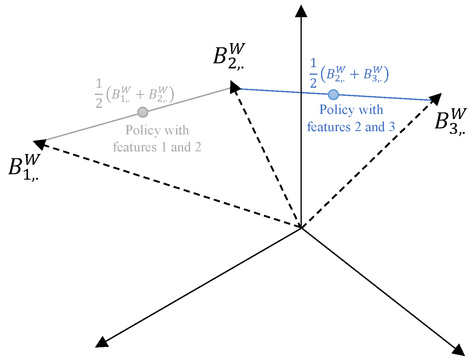
Since each modality $b=1,\dots ,m$ is represented by its corresponding row $r=1,\dots ,m$ in ${\mathit{B}}^{\mathit{W}}$, that is, by a vector in ${\mathbb{R}}^m$, each policy can be projected in Burt space by taking the center of gravity ${\mathit{D}}_{i,.}{\mathit{B}}^{\mathit{W}}/q$ of its modalities in ${\mathit{D}}_{i,.}$, whose Burt coordinates are stored in the corresponding rows of ${\mathit{B}}^{\mathit{W}}$. This is illustrated in Figure 1 in the case of three modalities.

Burt distance between the i-th and $i^{\prime }$-th policies is then given by:

$$d(i,i^{\prime })={∥{\mathit{D}}_{i,.}{\mathit{B}}^{\mathit{W}}/q-{\mathit{D}}_{i^{\prime },.}{\mathit{B}}^{\mathit{W}}/q∥}_2$$

(9)

We adapt the K-means Algorithm 1 to our Burt distance-based framework as follow. Each policy is projected into Burt space and identified by its center of gravity ${\mathit{D}}_{i,.}{\mathit{B}}^{\mathit{W}}/q$. The new centroids ${\mathit{c}}_u(e+1)$ of $S_u\left(e\right)$ are now defined by the following m-vector:

$${\mathit{c}}_u(e+1)={\displaystyle \frac{1}{|S_u\left(e\right)|}}\sum _{{\mathit{x}}_i\in S_u\left(e\right)}{\mathit{D}}_{i,.}{\mathit{B}}^{\mathit{W}}/q.$$

The Euclidean dissimilarity measure is replaced by Burt distance defined in Equation (9).

To benchmark our Burt distance-based K-means, we first implement K-modes on the categorical data (Gender, Zone, and Class) from the Wasa insurance dataset. The dissimilarity measure $d(.)$ in K-means Algorithm 1 is simply replaced by Hamming distance defined in Equation (5).

Table 4. Table summary of K-modes clustering results (policy allocation, dominant features, and average claim frequencies per cluster). K-modes (Hamming distance) applied on data characterized by three categorical variables.

Cluster	% of Policies	Gender	Zone	Class	Frequency (%)
6	2.82	K	4	5	0.6003
1	5.73	K	4	3	0.627
5	2.77	K	3	[3, 4]	0.7855
10	13.39	M	[2, 4]	4	0.8559
3	17.03	M	4	3	0.8919
2	20.61	M	3	3	0.9374
9	19.99	M	[3, 4]	5	1.0532
7	2.73	K	2	[3, 4]	1.2236
8	5.06	M	2	1	1.8256
4	9.88	M	[2, 4]	6	1.9443

reports the policy allocation, the dominant modalities, as well as the average claim frequency associated with each cluster. The dominant modality or modalities are identified as the dominant representative(s) in each cluster. A quick analysis reveals the most and least risky driver profiles. The riskiest category, with an average claim frequency of 1.94%, contains a majority of vehicles with the highest ratio of power (EV ratio 25–). The lowest claim frequencies (0.6–0.785%) correspond to a majority of women living in small towns or in the countryside (Zone 3 and 4).

If we use the average motor claim frequency per cluster as a predictor, ${\widehat{\lambda }}_i$, we can estimate the goodness of fit of the partition with the Poisson deviance defined in Equation (10). The deviance is the difference between the saturated and partitioned model’s log-likelihood. If $N_i$ and ${\nu }_i$ are, respectively, the number of claims and the duration (exposure) of the i-th contract, the deviance is defined as:

$$D^{*}=2\sum _{i=1}^n{N}_i\left({\displaystyle \frac{{\nu }_i}{N_i}}{\widehat{\lambda }}_i-\left(log{\displaystyle \frac{{\widehat{\lambda }}_i{\nu }_i}{N_i}}+1\right)I_{\{N_i\ge 1\}}\right)$$

(10)

The deviance, AIC, and BIC are reported in

Table 5. Statistics of goodness of fit obtained by partitioning the categorical data into 10 clusters with K-modes.

Goodness of Fit
Deviance	6576.31
AIC	8244.88
BIC	9691.58

. Both AIC and BIC are computed with a number of degrees of freedom equal to 10 × 16 (# of clusters × # of modalities).

We now implement our Burt distance-based K-means algorithm on the same categorical data (Gender, Zone, and Class).

Table 6. Table summary of Burt distance-based K-means clustering results (policy allocation, dominant features, and average claim frequencies per cluster). Burt distance-based K-means applied on data characterized by three categorical variables.

Cluster	% of Policies	Gender	Zone	Class	Frequency (%)
2	8.21	M	4	3	0.3811
9	12.27	M	4	[4, 5]	0.5051
1	8.95	M	6	[3, 5]	0.6808
4	6.43	K	4	[3, 5]	0.6813
7	4.58	M	2	3	0.8621
6	11.82	M	4	[1, 6]	0.9237
10	8.75	K	[2, 3]	[3, 4]	1.0144
5	16.81	M	3	[3, 5]	1.0825
3	10.94	M	2	[4, 6]	2.1482
8	11.23	M	1	[3, 4]	3.0878

reports the policy allocation, the dominant modalities, and the claim frequency associated with each cluster. For each cluster $S_u$, the dominant modalities are identified either as the cluster’s most common representatives, as in Table 4, or as the ones whose Burt coordinates are closest, in terms of the ${\ell }^2-\mathrm{norm}$, to the cluster center:

$$\underset{v\in \{1,\dots ,m_b\}}{arg min}{∥c_u-B_{{\sum }_{d=1}^{b-1}{m}_d+v,.}^W∥}_2$$

The average claim frequency per cluster is more heterogeneous (from 0.38% up to 3.08%) compared to what we obtained in Table 4 (0.62–1.94%). The most and least risky driver profiles also seem to be more clearly defined. The riskiest category, with an average claim frequency (of around 3%), much higher than the one obtained with Hamming distance, contains a majority of vehicles in central and semi-central parts of Sweden’s three largest cities (Zone 1). The cluster with the second-highest claim frequency (on average) also has a majority of vehicles with high power (Classe 4–6) driven in suburbs plus middle-size cities (Zone 2), whereas the lowest claim frequencies are characterized by vehicles in small towns and the countryside (Zone 4 and 6).

The Deviance, AIC, and BIC are reported in

Table 7. Statistics of goodness of fit obtained by partitioning the categorical data into 10 clusters with Burt distance-based K-means.

Goodness of Fit
Deviance	6350.04
AIC	8018.61
BIC	9465.31

. Both AIC and BIC are computed with a number of degrees of freedom equal to 10 × 16 (# of clusters × # of modalities). The goodness of fit is clearly better than the one obtained using K-modes with Hamming distance in Table 5.

2.3. Burt Distance for Mixed Data Types

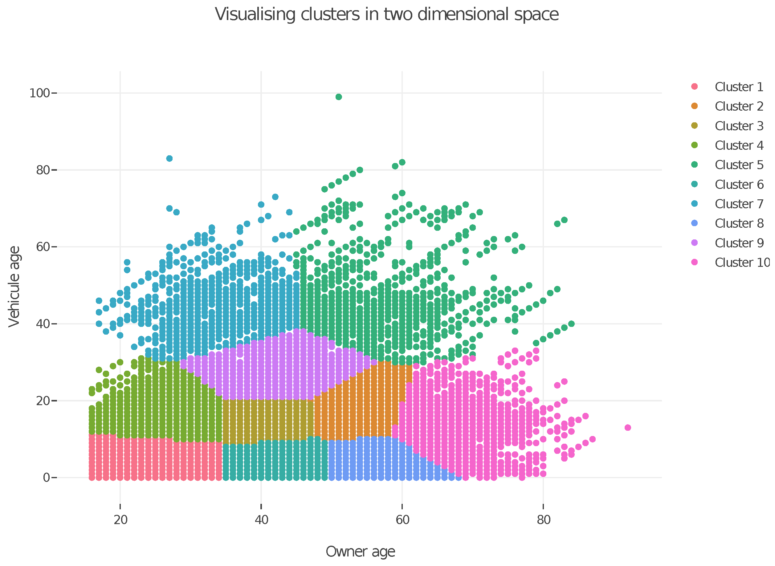
We have both theoretically and empirically demonstrated that Burt distance is a favorable alternative to Hamming distance for clustering categorical data. In the following, we demonstrate that our Burt distance-based approach also improves the partition quality when handling heterogeneous datasets, outperforming K-prototypes and K-medoids. We first empirically illustrate, with the standard K-means algorithm, that the unsupervised discretization of continuous variables, required with our Burt approach, does not negatively affect the method’s goodness of fit. Accordingly, we apply the standard K-means algorithm on the numeric rating factors (owner’s age and vehicle age) from the Wasa insurance dataset. The Deviance, AIC, and BIC are reported in

Table 8. Statistics of goodness of fit obtained by partitioning the numeric data into 10 clusters with the K-means algorithm (using Euclidean distance).

Goodness of Fit
Deviance	6097.18
AIC	7485.75
BIC	7666.59

. Both AIC and BIC are computed with a number of degrees of freedom equal to 10 × 2 (# of clusters × # of numeric variables). Figure 2 displays the 10 clusters in a two-dimensional space with the owner’s and vehicle’s ages on the axes.

Table 9. Table summary of K-means clustering results (policy allocation, dominant features, and average claim frequencies per cluster). K-means applied on data characterized by two continuous variables.

Cluster	% of Policies	Gender	Zone	Class	Owner Age	Vehicle Age	Frequency (%)
5	2.00	M	[3, 4]	1	[48, 62]	[38, 48]	0
9	4.85	M	[3, 4]	[3, 4]	[40, 48]	[21, 26]	0.2035
2	15.16	M	[3, 4]	[3, 5]	[48, 53]	[13, 17]	0.3698
10	6.46	M	[3, 4]	[3, 5]	[60, 66]	[12, 18]	0.45
3	14.94	M	[3, 4]	[3, 5]	[42, 47]	[13, 17]	0.51
7	2.09	M	[2, 4]	1	[28, 43]	[37, 48]	0.5106
6	13.54	M	[2, 4]	[3, 4]	[44, 49]	[1, 5]	0.8667
8	11.65	M	[2, 4]	[3, 4]	[50, 55]	[1, 5]	0.9183
4	14.42	M	[2, 4]	[3, 5]	[25, 32]	[12, 16]	1.5317
1	14.89	M	[2, 4]	[3, 6]	[23, 29]	[1, 7]	4.1332

reports the claim frequency, the percentage of policies, as well as the dominant modalities associated to each cluster. The riskiest category, with an average claim frequency of around 4%, is characterized by young/less experienced drivers (aged between 23 and 29) of recent vehicles with high ratio powers (class 3 to 6), whereas the cluster with the smallest claim frequency (around 0%) is made up of middle-aged (48–62 years old) males driving classic cars (38+ years old) with low ratio power (class 1). We can also observe that the clusters with the lowest claim frequencies have a majority of insured living in lesser/small towns or the countryside (Zones 3 and 4), while clusters with the highest claim frequencies have, in addition, a majority of insured living in the suburbs or middle-sized cities (Zone 2).

To apply our Burt distance-based K-means on continuous variables, we first have to discretize them. We categorized the owner’s age and the age of their vehicle into four and three categories, respectively: $[16,35)[35,47)[47,58)[58,93)$ for owner’s age and $[0,11)[11,29)[29,100)$ for vehicle’s age. This discretization was performed using the univariate K-means algorithm. The use of this unsupervised discretization approach is justified by the non-normality of the numeric variables’ distribution and the existence of outliers (especially in the vehicle age variable). While this univariate discretization does not account for potential interactions between rating factors, projecting the discretized data into Burt space helps address this concern. The deviance reported in

Table 10. Statistics of goodness of fit obtained by partitioning the discretized numeric data (projected in Burt space) into 10 clusters with the Burt distance-based K-means algorithm.

Goodness of Fit
Deviance	6097.51
AIC	7586.08
BIC	8219.01

is approximately the same as the one obtained in Table 8, where the standard K-means algorithm was applied to the non-discretized numeric data. The Burt framework’s capacity to capture dependencies between modalities through the analysis of joint frequencies appears to offset the risk of information loss inherent to such an unsupervised discretization. Both the AIC and BIC are computed with 10 × 7 degrees of freedom (# of clusters × # of modalities). For comparison, the residual deviance of a GLM model fitted to the same categorical classes is equal to $6094.49$. Figure 3 displays the 10 clusters in a two-dimensional space. The hard-edge cutoffs observed in Figure 3 are an effect of the discretization process.

Table 11. Table summary of Burt distance-based K-means clustering results (policy allocation, dominant features, and average claim frequencies per cluster). Burt distance-based K-means applied on data characterized by two discretized continuous variables.

Cluster	% of Policies	Gender	Zone	Class	Owner Age	Vehicle Age	Frequency (%)
9	2.66	M	[3, 4]	1	[35, 46]	[29, 46]	0.2207
10	2.76	M	[2, 4]	1	[29, 52]	[29, 45]	0.3083
3	15.31	M	[3, 4]	[3, 5]	[47, 52]	[13, 17]	0.3257
2	15.23	M	[3, 4]	[3, 5]	[42, 46]	[12, 17]	0.408
7	6.41	M	[3, 4]	[3, 5]	[58, 63]	[13, 17]	0.456
6	12.96	M	[2, 4]	[3, 5]	[47, 52]	[1, 6]	0.906
5	10.46	M	[2, 4]	[3, 4]	[42, 46]	[1, 5]	0.915
8	4.69	M	[2, 4]	[3, 4]	[58, 62]	[1, 5]	0.9444
4	14.32	M	[2, 4]	[3, 5]	[25, 32]	[12, 16]	1.5324
1	15.21	M	[2, 4]	[3, 6]	[23, 29]	[1, 7]	4.0664

reports the claim frequency, the percentage of policies, as well as the dominant modalities associated to each cluster. The policy allocation (in the second column) as well as the two riskiest categories are very similar to those obtained in Table 9. However, we do observe small differences. For instance, our Burt-adapted K-means seems to better identify the link between low ratio power and smaller claim frequencies. The clusters with the two lowest claim frequencies are indeed the only ones labeled with class 1 (the lowest class of ratio power), which was not the case in Table 9.

We assess the discretization required by our Burt framework on a simulated dataset to further validate our findings. We generate 1000 observations from two continuous variables $X_1$ and $X_2$. The simulated data points, illustrated in Figure 4, are such that we can visually identify two distinct clusters. We categorize each variable, as required by our Burt approach, with the standard K-means algorithm (unsupervised approach) in 10 categories. We then apply our Burt distance-based K-means to the discretized data. Figure 4 shows that our Burt approach was effectively able to identify the two clusters.

We can now benchmark our Burt distance-based K-means against K-prototypes (linear combination of Euclidean and Hamming distances) and K-medoids (Gower distance). Huang (1998) extended K-modes (Huang 1997) to handle mixed data types with the K-prototypes algorithm. This hybrid method combines K-means and K-modes by using a weighted sum of Euclidean distance for numeric data and Hamming distance for categorical data:

$$d({\mathit{x}}_i,{\mathit{c}}_u)=\sum _{j=1}^p{\left(x_{i,j}-c_{u,j}\right)}^2+\beta \left(\sum _{b=1}^m\mathbf{1}\{{\mathrm{x}}_{\mathrm{i},\mathrm{b}}\ne {\mathrm{c}}_{\mathrm{u},\mathrm{b}}\}\right),$$

where $\beta \in {\mathbb{R}}^{+}$ is a weighted factor that controls the relative importance of categorical variables with respect to numerical ones.

Table 12. Statistics of goodness of fit obtained by partitioning the mixed-type dataset into 15 clusters with the K-prototypes algorithm.

Goodness of Fit
Deviance	6161.47
AIC	8050.04
BIC	10,491.35

presents the clustering results obtained by applying K-prototypes with $\beta =1$ to the Wasa insurance portfolio, which contains two continuous and three categorical features. As reported in

Table 13. Table summary of K-prototypes clustering results (dominant features and average claim frequencies per cluster).

Cluster	% of Policies	Gender	Zone	Class	Owner Age	Vehicle Age	Frequency (%)
13	4.45	M	4	[1, 4]	[39, 51]	[23, 30]	0.1754
5	3.50	M	[3, 4]	1	[30, 53]	[38, 46]	0.228
15	7.94	M	3	3	[43, 53]	[13, 19]	0.301
11	9.28	M	4	3	[51, 62]	[1, 16]	0.3856
14	9.24	M	4	5	[43, 55]	[12, 17]	0.3888
4	5.07	M	4	2	[45, 60]	[13, 19]	0.5943
12	5.82	K	4	[3, 4]	[33, 46]	[12, 18]	0.5985
7	9.01	M	[2, 3]	4	[43, 52]	[1, 17]	0.6748
2	4.56	K	[1, 2]	3	[24, 48]	[1, 16]	1.2525
6	4.85	M	[2, 6]	6	[45, 54]	[1, 8]	1.3813
9	5.30	M	4	[1, 4]	[18, 29]	[12, 17]	1.5103
1	7.37	M	1	3	[39, 50]	[0, 15]	1.6583
3	8.41	M	4	3	[21, 29]	[1, 6]	2.266
8	8.57	M	2	5	[24, 34]	[1, 17]	2.5845
10	6.63	M	3	6	[23, 29]	[6, 13]	3.8295

, the riskiest cluster is once again characterized by younger drivers of vehicles with high power-to-weight ratios (classes 5 and 6), while the cluster with the lowest claim frequencies consists mainly of ancient vehicles (23+). Nevertheless, no clear patterns seem to emerge from the cluster analysis, and the deviance, in Table 12, is worse than the one obtained when clustering only quantitative variables. One can eventually consider adjusting $\beta$ in order to minimize the deviance, but we failed to find a value of $\beta$ that significantly improved the results for the Wasa dataset.

We further benchmark our Burt-distance based K-means for mixed data types with K-medoids (Kaufman and Rousseeuw 2009). Unlike K-means, it selects actual data points (medoids) as the cluster centers, making it more robust to noise and outliers. When dealing with mixed data types (numerical and categorical), Gower distance is commonly used as the K-medoids dissimilarity measure. It computes the distance between two objects as a combination of dissimilarities across all variable types. Formally, Gower distance is defined as:

$$d\left({\mathit{x}}_i,{\mathit{x}}_j\right)={\displaystyle \frac{1}{f}}\sum _{g=1}^f{\delta }_{i,j}^{\left(g\right)}{d}_{i,j}^{\left(g\right)},$$

where f denotes the number of features, $d_{i,j}^{\left(g\right)}$ is the normalized distance for the g-th feature, and ${\delta }_{i,j}^{\left(g\right)}$ is an indicator function that equals 1 if the g-th feature is comparable for both observations, and 0 otherwise.

Gower distance requires computing pairwise dissimilarities between all data points in the dataset. For a dataset with n observations, this results in the calculation of ${\displaystyle \frac{1}{2}}n\left(n-1\right)$ pairwise distances, which scales quadratically with the size of the dataset. When working with an insurance portfolio, this rapidly becomes computationally prohibitive. On the Wasa insurance dataset, computing the Gower distance matrix took approximately 25 min. The exhaustive search for optimal medoids, and the complexity of handling mixed data types, led to an additional 26 min to run the K-medoids algorithm with the pre-computed distances. Moreover, the resulting deviance, in

Table 14. Statistics of goodness of fit obtained by partitioning the mixed-type dataset into 15 clusters with the K-medoids algorithm (using Gower distance).

Goodness of Fit
Deviance	6290.92
AIC	8179.49
BIC	10,620.80

, is even worse than the one obtained with K-prototypes in Table 12.

The disappointing results obtained with K-prototypes and K-medoids lead us now to apply our Burt distance-based K-means on the Wasa insurance dataset with two discretized continuous variables and three categorical variables. As reported in

Table 15. Table summary of Burt distance-based K-means on mixed data types (dominant features and average claim frequencies per cluster).

Cluster	% of Policies	Gender	Zone	Class	Owner Age	Vehicle Age	Frequency (%)
13	4.83	M	[3, 4]	1	[35, 55]	[29, 46]	0.2512
2	9.86	M	4	[4, 5]	[40, 52]	[12, 17]	0.3141
3	9.52	M	[1, 3]	[3, 5]	[47, 52]	[13, 17]	0.3225
10	7.60	M	[2, 3]	[3, 5]	[42, 46]	[12, 17]	0.4842
9	8.09	K	[3, 4]	[3, 5]	[25, 51]	[13, 17]	0.5647
5	5.77	M	4	[3, 5]	[47, 55]	[1, 6]	0.5936
7	9.19	M	[3, 4]	[3, 5]	[58, 62]	[1, 17]	0.6645
8	4.23	M	4	[3, 5]	[25, 34]	[11, 16]	0.8449
4	6.46	M	[1, 3]	[3, 4]	[42, 46]	[1, 5]	1.0119
12	6.83	K	[3, 4]	[3, 4]	[24, 52]	[1, 6]	1.2278
15	7.23	M	[2, 3]	[3, 4]	[47, 52]	[1, 5]	1.2402
11	5.80	M	[2, 3]	[3, 6]	[24, 31]	[11, 15]	2.0485
6	4.38	M	4	[3, 6]	[22, 29]	[1, 7]	2.3001
14	6.56	M	[2, 3]	[3, 6]	[23, 29]	[1, 8]	4.2849
1	3.66	M	1	[3, 4]	[25, 31]	[1, 9]	8.084

, we obtain a greater heterogeneity between clusters with an average claim frequency ranging from 0.25% up to 8%. The first four riskiest categories are characterized by a majority of young drivers (between roughly 22 and 29 years old). The differences in the vehicle ages are also more defined between clusters, with the oldest vehicles assigned to the cluster with the smallest claim frequency, and more recent vehicles assigned to clusters with higher claim frequencies. Vehicles with the lowest power ratio (Class 1) are also exclusively represented in the cluster (13) with the smallest claim frequency, whereas vehicles with the highest power ratio (class 6) are only represented in clusters (11, 6, and 14) with higher claim frequencies. The cluster (1) with the highest claim frequency is also exclusively labeled with vehicles in central and semi-central parts of Sweden’s three largest cities (Zone 1). On a side note, the under-representation of female drivers in the portfolio is also reflected in the dominant gender (mostly men) associated with each cluster.

The Deviance, AIC, and BIC are reported in

Table 16. Statistics of goodness of fit obtained by partitioning the mixed-type dataset into 15 clusters with the Burt distance-based K-means algorithm.

Goodness of Fit
Deviance	5978.96
AIC	8017.53
BIC	11,136.99

. Both AIC and BIC are computed with 20 × 23 degrees of freedom (# of clusters × # of modalities). The deviance, measuring our model’s goodness of fit, is clearly better than the one obtained with K-prototypes or K-medoids. In comparison, the deviance of a GLM model fitted to the same dataset is around 5824.

Note that we chose the number of clusters K based on the marginal gain of intra-class inertia and the marginal reduction in deviance. As illustrated in Figure 5, the marginal gain of inertia (or reduction in deviance)—averaged over fifteen seed values—is limited above a certain number of clusters. Given the size of our motorcycle portfolio (60,000+ policies), we chose $K=15$ in order to get closer to the GLM deviance ($5823.66$) while still effectively summarizing the large amount of information in our data.

3. Burt-Adapted K-Means Variants

In this section, we extend the scope of application of our Burt framework to K-means variants, namely the mini-batch and fuzzy K-means. The mini-batch extension is particularly suited to address computational challenges associated with large-scale data, a common issue with insurance datasets, whereas fuzzy K-means is a soft form of clustering (each object can belong to multiple clusters).

3.1. Mini-Batch K-Means

The K-means algorithm stores the entire dataset in main memory, which can become computationally costly when handling large datasets. The mini-batch K-means algorithm was proposed as a solution by Sculley (2010). This extension utilizes small random batches of data with a fixed size. In each iteration, a new random sample from the dataset is used to update the clusters. This process continues until convergence. The specifics of how we adapted the mini-batch variant to our Burt framework are outlined in Algorithm 3.

Empirical evidence in the literature suggests a substantial reduction in computational time, though often at the expense of partition quality. Figure 6 compares the running time, with respect to the number of clusters, of our Burt-adapted K-means with its mini-batch extension. While the discrepancy in partition quality (between the standard K-means and its mini-batch variant) remains small, the difference in computational time grows noticeably. The mini-batch algorithm exhibits a relatively stable runtime, while K-means becomes increasingly time-consuming. However, the overall gain in computation time is still limited (both algorithms complete within a few seconds). To observe significant gains in computation time, mini-batch K-means would need to be tested on a larger dataset than the Wasa dataset used here.

Algorithm 3: Mini-batch K-means algorithm.

We applied the mini-batch algorithm to the Wasa dataset using Burt distance (defined in Equation (9)) with batch sizes of 5000 policies. As described in Section 2.3, continuous variables are discretized.

Table 17. Burt-adapted mini-batch clustering. Policy allocation, dominant features, and average claim frequencies per cluster.

Cluster	% of Policies	Gender	Zone	Class	Owner Age	Vehicle Age	Frequency (%)
6	3.71	M	4	1	[35, 64]	[13, 48]	0.2625
11	7.94	M	4	[3, 4]	[47, 59]	[12, 17]	0.2759
2	3.31	M	[1, 3]	1	[29, 60]	[29, 45]	0.4523
10	6.91	M	4	[5, 6]	[22, 46]	[12, 16]	0.5052
15	6.77	M	[1, 4]	[3, 4]	[42, 46]	[12, 17]	0.5295
8	8.06	K	[3, 4]	[3, 5]	[25, 51]	[13, 17]	0.5661
5	9.85	M	4	3	[47, 55]	[1, 5]	0.656
9	8.58	M	[1, 2]	[3, 6]	[47, 54]	[13, 17]	0.7156
3	5.44	M	3	3	[23, 63]	[13, 17]	0.7496
14	8.26	M	[2, 4]	[3, 5]	[42, 46]	[1, 6]	0.9482
12	5.58	M	[2, 3]	5	[24, 52]	[13, 17]	1.0196
7	6.82	K	[3, 4]	[3, 4]	[24, 52]	[1, 6]	1.2301
4	5.81	M	[2, 3]	[4, 5]	[47, 53]	[1, 7]	1.6504
1	4.89	M	4	[4, 6]	[22, 28]	[5, 10]	3.2768
13	8.07	M	[1, 3]	[3, 5]	[23, 29]	[1, 6]	5.9861

presents the results for 15 centroids. The mini-batch K-means runs faster and gives approximately the same results. We observe more or less the same dominant modalities discovered in Table 15. The deviance, reported in

Table 18. Statistics of goodness of fit obtained by partitioning the dataset into 15 clusters with the Burt-adapted mini-batch K-means.

Goodness of Fit
Deviance	6049.68
AIC	8088.25
BIC	11,207.71

, is slightly higher than that of a segmentation based on the Burt-adapted K-means algorithm. Note that this minor reduction in cluster quality may be due to the increased presence of noise in the mini-batch algorithm.

3.2. Fuzzy K-Means

The K-means algorithm, often referred to as “hard clustering”, attempts to partition a dataset into K distinct clusters. Each data point is assigned to the cluster whose center is the nearest and may only belong to one cluster. In contrast, the fuzzy K-means algorithm proposed by Dunn (1973) and later improved by Bezdek et al. (1984) is known as “soft clustering”, as it allows data points to belong to more than one cluster. Given a finite set of data, the algorithm returns two outputs: a set of K cluster centers $\{{\mathit{c}}_1,\dots ,{\mathit{c}}_K\}$, and a partition matrix W, which contains the membership values $w_{i,k}$ for $i=1,\dots ,n$ and $k=1,\dots ,K$. Like K-means, fuzzy K-means aims to minimize the intra-cluster variance:

$$arg min\sum _{i=1}^n\sum _{k=1}^K{\left(w_{i,k}\right)}^{m}d(i,{\mathit{c}}_k),$$

where

$$w_{i,k}={\displaystyle \frac{1}{{\sum }_{u=1}^K{\left(\frac{d(i,{\mathit{c}}_k)}{d(i,{\mathit{c}}_u)}\right)}^{\frac{2}{m-1}}}}.$$

The hyper-parameter $m\in {\mathbb{R}}^{+}$ determines the level of cluster fuzziness. A large m results in smaller membership grades $w_{i,k}$, and hence fuzzier clusters. In the limit $m=1$, the memberships, $w_{i,u}$, converge to 0 or 1, which amounts to crisp partitioning.

The arbitrary centroid initialization and the pre-specified number of clusters both retain their significant influence over the final partition. The Burt-adapted fuzzy K-means is detailed in Algorithm 4.

Algorithm 4: Fuzzy clustering.

We apply the Burt-adapted fuzzy K-means to the Wasa insurance dataset. We once again discretize the continuous variables as explained in Section 2.3. We run the algorithm with a fuzziness parameter of $m=1.20$. The policies are assigned to the most likely cluster (highest $w_{i,k}$ for $k=1,\dots ,K$).

Table 19. Burt-adapted fuzzy clustering. Policy allocation, dominant features, and average claim frequencies per cluster.

Cluster	% of Policies	Gender	Zone	Class	Owner Age	Vehicle Age	Frequency (%)
2	5.16	M	4	[3, 5]	[47, 52]	[12, 17]	0.2604
7	4.72	M	[3, 4]	1	[35, 60]	[29, 46]	0.2992
14	8.21	M	[2, 3]	[3, 5]	[47, 52]	[13, 17]	0.3552
6	4.92	M	4	[3, 5]	[41, 46]	[12, 18]	0.3586
9	6.02	M	[3, 4]	[3, 5]	[58, 63]	[13, 17]	0.449
12	7.6	M	[2, 3]	[3, 5]	[42, 46]	[12, 17]	0.4842
4	3.78	M	[2, 4]	3	[47, 52]	[1, 5]	0.6654
10	4.4	M	[2, 4]	[3, 4]	[58, 62]	[1, 5]	0.8285
1	4.23	M	4	[3, 5]	[25, 34]	[11, 16]	0.8449
11	14.88	K	[3, 4]	[3, 4]	[24, 51]	[1, 17]	0.8598
3	8.47	M	[2, 4]	[3, 5]	[42, 46]	[1, 6]	0.934
5	7.29	M	[2, 4]	[4, 5]	[47, 52]	[1, 7]	1.0891
13	4.44	M	4	[3, 6]	[22, 29]	[1, 7]	2.2784
15	7.08	M	[2, 3]	[3, 5]	[25, 32]	[11, 15]	2.4298
8	8.8	M	[2, 3]	[3, 6]	[23, 29]	[1, 7]	5.7983

reports the most frequent features and the average claim frequency in each cluster. We find similar profiles to those found in Table 15 with more recent (older) vehicles with higher (lower) ratio power driven by younger (older) policyholders in clusters with higher (lower) claim frequencies on average.

The deviance, in

Table 20. Statistics of goodness of fit obtained by partitioning the dataset into 15 clusters with the Burt-adapted fuzzy K-means.

Goodness of Fit
Deviance	6026.25
AIC	8064.82
BIC	11,184.27

, is better than that of the mini-batch K-means, and remains quite close to the one obtained with our Burt-adapted K-means. On a side note, if we set $m=2$, which is a standard level of fuzziness in the literature, several clusters are not assigned any policies, but some policies have a non-null probability of belonging to them.

4. Burt-Adapted Spectral Clustering

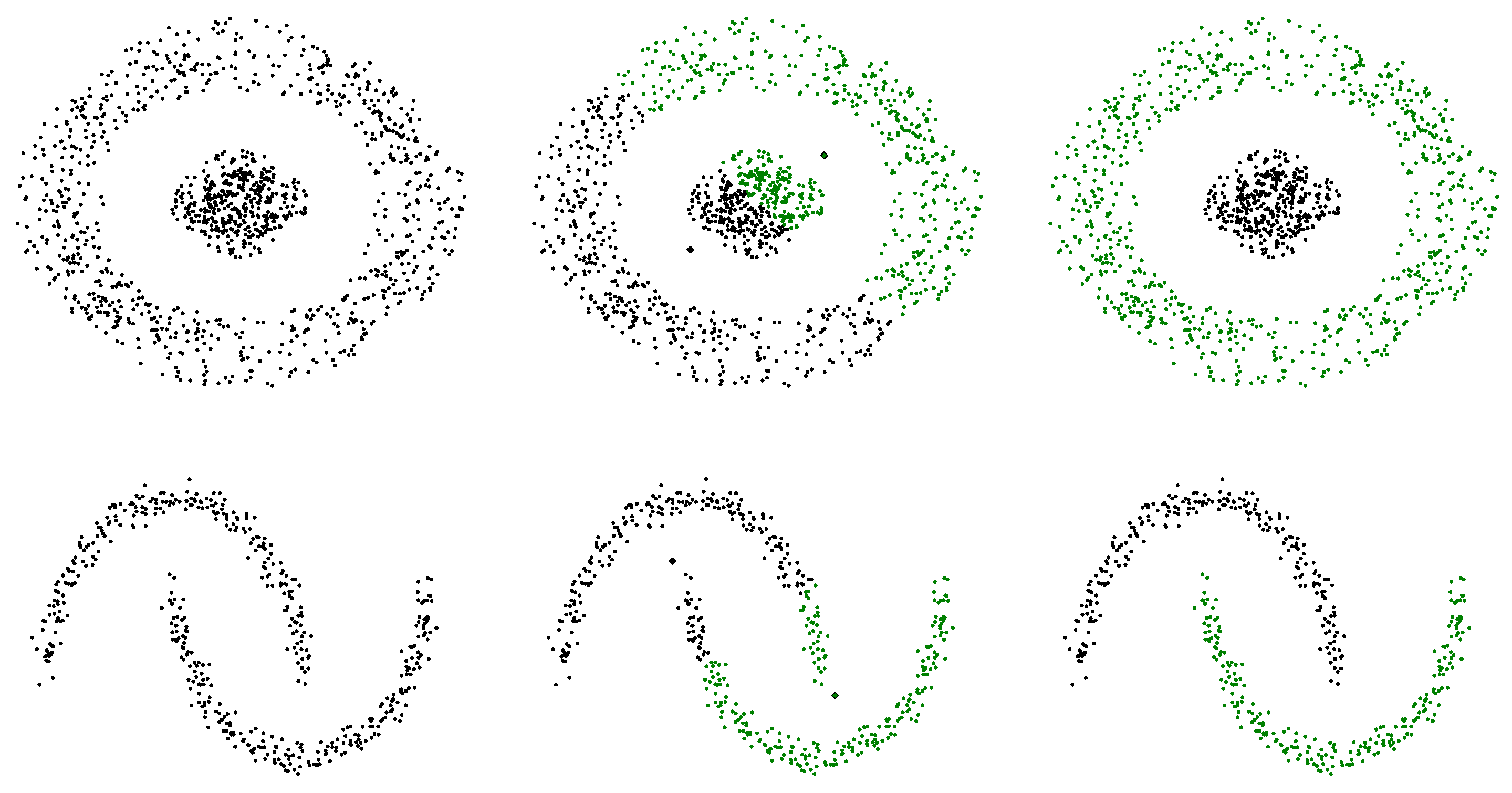
Since K-means relies on Euclidean distance, each iteration partitions the space into (hyper)spherical clusters. This makes K-means unsuitable for detecting clusters with non-convex shapes. For example, in Figure 7, K-means fails to distinguish the inner and outer rings or the upper and lower moons of the circular and moon-shaped data. This poor clustering performance stems from the fact that the natural clusters do not form convex regions.

By exploiting a deeper data geometry, spectral clustering (Belkin and Niyogi 2001; Ng et al. 2001; Shi and Malik 2000) addresses the lack of flexibility of K-means in cluster boundaries. While K-means attempts to associate each cluster with a hard-edged sphere, spectral clustering embeds the data into a new space derived from a graphical representation of the dataset. Applying the K-means algorithm to this representation bypasses the spherical limitation, and results in the intended non-convex cluster shapes.

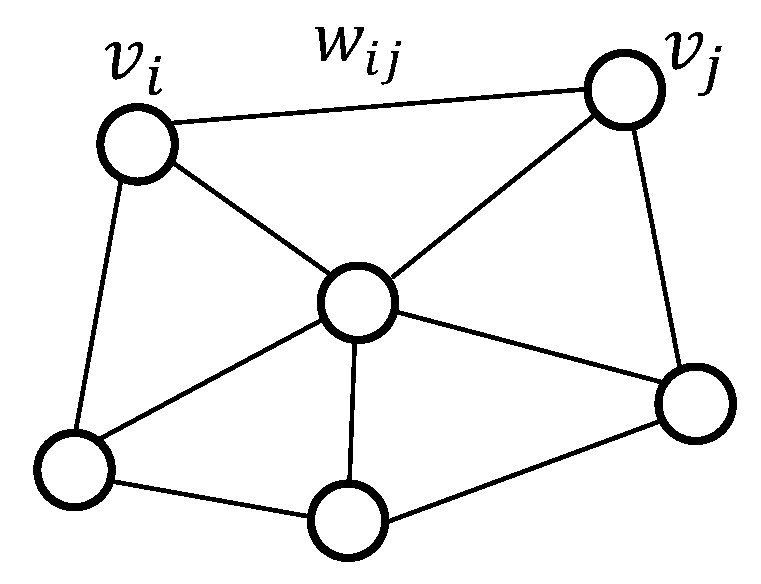
The graph theory is the core component in the graph representation of the dataset. As illustrated in Figure 8, an undirected graph $G=(V,E,W)$ is defined by three elements:

• a set of vertices $V={\left\{v_i\right\}}_{i=1,\dots ,n}$ where each vertex $v_i$ represents one of the n data points in the dataset;
• a set of edges $E=\{e_{i,j}:v_i⟷v_j\}$ whose entries are equal to 1 if two vertices $v_i$ and $v_j$ are connected by an undirected edge $e_{i,j}$, and 0 otherwise;
• a set of weights $W=\{w_{ij}:w_{ij}\ne 0\mathrm{if}{v}_i⟷v_j\}$ that contains the similarity between two vertices linked by an edge.

E and W can both be represented as $n\times n$ matrices. The matrix W is often referred to as the weighted adjacency matrix A.

The dataset $X=\{{\mathit{x}}_1,\dots {\mathit{x}}_n\}$, where ${\mathit{x}}_i\in {\mathbb{R}}^p$ can thence be represented as a graph $G=(V,E,W)$ by first associating each data point $x_i$ with a vertex $v_i$. A measure of similarity is then defined between two data points i and j. A common choice is the Gaussian kernel:

$$S(i,j)=exp\left(-{\displaystyle \frac{d(i,j)}{\alpha }}\right),$$

where $\alpha \in {\mathbb{R}}^{+}$ is a tuning parameter. Two highly similar data points are connected by an edge $e_{i,j}$ with a weight $w_{ij}$ equal to their similarity measure, while data points with low similarity are considered disconnected. Various methods exist for constructing a pairwise similarity graph, including (Hainaut and Thomas 2022):

• The $ϵ$-neighborhood graph: Points are connected if the pairwise distance between them is smaller than a threshold $ϵ$. In practice, we keep all similarities smaller than $exp\left(-{\displaystyle \frac{ϵ}{\alpha }}\right)$, while setting others to zero.
• The (mutual) k-nearest neighbor graph: The vertex $v_i$ is connected to vertex $v_j$ if $v_j$ is among the k-nearest neighbors of $v_i$. Since the neighborhood relationship is not symmetric, and the graph must be symmetric, we need to enforce the symmetry. The graph is made symmetric by ignoring the directions of the edges, i.e., by connecting $v_i$ and $v_j$ if either $v_i$ is among the k-nearest neighbors of $v_j$ or $v_j$ is among the k-nearest neighbors of $v_i$, resulting in the k-nearest neighbor graph. Alternatively, the connection is made if $v_i$ and $v_j$ are mutual k-nearest neighbors, resulting in the mutual k-nearest neighbor graph.
• The fully connected graph: All points in the dataset are connected.

Note that the choice of rule for constructing the graph influences the edge matrix and and may affect the resulting clusters.

To work with the graph representation, we apply the graph Fourier transform, which is based on the graph’s Laplacian representation. The Laplacian of a graph G is given by the difference between its degree matrix D and adjacency matrix A:

$$L=D-A$$

But why is matrix L called a graph Laplacian? We can understand this by defining a function on the vertices of the graph, $f:V\to \mathbb{R}$ such that each vertex is mapped to a value, $v_i\to f\left(v_i\right)$. Consider a discrete periodic function that takes N values at times $1,2,\dots ,N$. This periodic structure can be represented by a ring graph, as depicted in Figure 9, where the function wraps around to reflect the periodicity.

In order to find the Laplacian representation, we subtract the adjacency matrix A from the diagonal degree matrix D. The matrix D contains on its diagonal the degree of each vertex $D_{ii}$ = ${\sum }_j{w}_{i,j}$. The degree of a vertex $v_i$ represents the weighted number of edges connected to it and is equal to the sum of the row i in the adjacency matrix. The entries of the matrix A indicate the absence or presence of a (weighted) edge between the vertices. In this particular case, none of the vertices have edges to themselves, so its diagonal elements are 0. Because our graph is undirected, $E_{ij}=E_{ji}$. Both the adjacency and degree matrices are encased in the resulting Laplacian matrix; the diagonal entries are the degrees of the vertices, and the off-diagonal elements are the negative edge weights:

$$L=\left(\begin{array}{cccccc}2& 0& 0& 0& 0& 0\\ 0& 2& 0& 0& \ddots & 0\\ 0& 0& 2& 0& 0& ⋮\\ ⋮& \ddots & \ddots & \ddots & \ddots & ⋮\\ ⋮& \ddots & \ddots & 0& 2& 0\\ 0& 0& \dots & 0& 0& 2\end{array}\right)-\left(\begin{array}{cccccc}0& 1& 0& 0& 0& 0\\ 1& 0& 1& 0& \ddots & 0\\ 0& 1& 0& 1& 0& ⋮\\ ⋮& \ddots & \ddots & \ddots & \ddots & ⋮\\ ⋮& \ddots & \ddots & 1& 0& 1\\ 1& 0& \dots & 0& 1& 0\end{array}\right)=\left(\begin{array}{cccccc}2& -1& 0& \dots & 0& -1\\ -1& 2& -1& 0& \ddots & 0\\ 0& -1& 2& -1& 0& ⋮\\ ⋮& \ddots & \ddots & \ddots & \ddots & ⋮\\ ⋮& \ddots & \ddots & -1& 2& -1\\ -1& 0& \dots & 0& -1& 2\end{array}\right)$$

Let $\mathit{f}={\left(f\left(v_j\right)\right)}_{j=1,\dots ,N}$ represent the vector of function values evaluated at the vertices of a graph G. The product $L\mathit{f}$, where L is the graph Laplacian, corresponds precisely to the second-order finite difference derivative of the function $f(.)$. This operation plays a key role in analyzing the graph’s structure, as the partitioning of the graph (including determining the number of clusters) can be inferred from the eigenvalues and eigenvectors of the graph Laplacian matrix, a process known as spectral analysis.

Since L is a symmetric matrix, it can be decomposed using eigenvalue decomposition as $L=U\Sigma U^{\top }$, where U is the matrix of eigenvectors, and $\Sigma$ is a diagonal matrix containing the eigenvalues. As the Laplacian is positive semi-definite, it can be easily shown that the smallest eigenvalue of L is always zero.

The analysis of the eigenvalues provides useful insights into the graph’s structure. Specifically, the multiplicity of the zero eigenvalue reflects the number of disconnected components in the graph, giving a way to partition the graph. For instance, if all vertices are disconnected, all eigenvalues will be zero. As edges are added, some eigenvalues become non-zero, and the number of zero eigenvalues corresponds to the number of connected components in the graph. To illustrate this, consider the graph in Figure 10, composed of K disconnected sub-graphs. In this case, the Laplacian matrix will have K zero eigenvalues, indicating that the graph consists of K independent components.

Beyond identifying the number of connected components, the eigenvalues of the graph Laplacian provide information about the density of the connections. The smallest non-zero eigenvalue, known as the spectral gap, indicates the overall connectivity density of the graph. A large spectral gap suggests a densely connected graph, while a small spectral gap implies that the graph is close to being disconnected. Thus, the first positive eigenvalue offers a continuous measure of the graph’s connectedness.

The second smallest non-zero eigenvalue, often referred to as the Fiedler value or the algebraic connectivity, is particularly useful for partitioning the graph. This value approximates the minimum graph cut required to divide the graph into two connected components. For example, if the graph consists of two groups of vertices, $V_1$ and $V_2$, connected by an additional edge (as shown in Figure 11), vertices $v_1$ and $v_2$ on either side of the cut can be assigned to $V_1$ or $V_2$ by analyzing the values in the Fiedler vector.

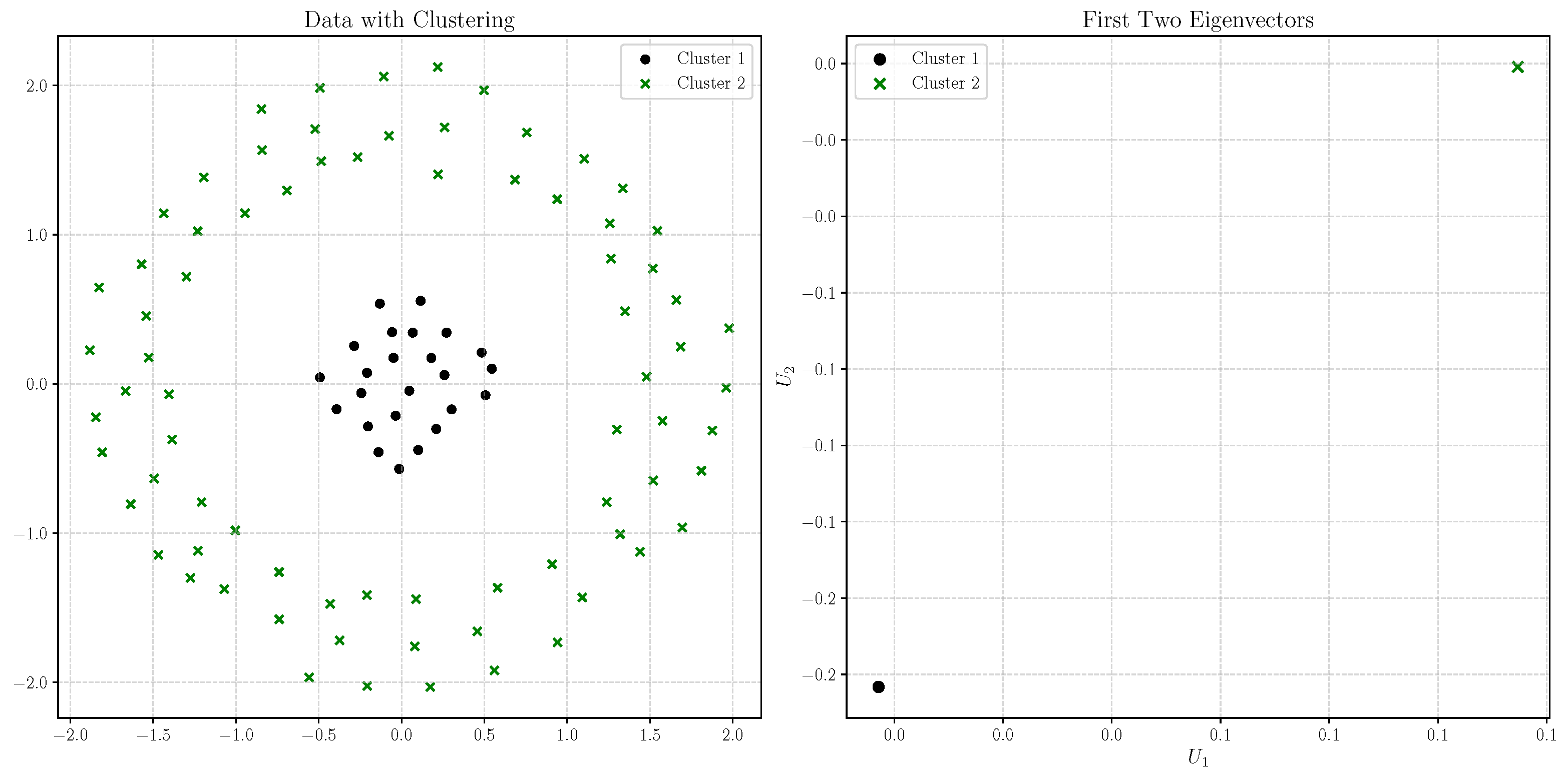
If a graph consists of K disconnected sub-graphs, it can be shown that the elements of the K eigenvectors with null eigenvalues are approximately constant over each cluster. In other words, the eigenvectors’ coordinates of points belonging to the same cluster are identical. Intuitively, since the eigenvectors of zero tell us how to partition the graph, the first K columns of U (the eigenvectors’ coordinates) consist of the cluster indicator vectors. Let us assume two well-separated sub-graphs. The eigenvectors’ coordinates ${(U_{i,1},U_{i,2})}_{i=1,\dots ,n}$ with a null eigenvalue are constant for all vertices $v_i$ belonging to the same sub-graph $V_k$. Formally, for $K=2$, we have ${(U_{i,1},U_{i,2})}_{i=1,\dots ,n}=(U_{k,1},U_{k,2})\forall v_i\in V_k,k=1,2$. The proof is detailed in Appendix A. If the K clusters are not identified, K-means can be applied to the rows of the first K eigenvectors, as these rows can serve as representations of the vertices. The complete procedure is outlined in Algorithm 5 (Von Luxburg 2007) from Hainaut and Thomas (2022).

Algorithm 5: Spectral clustering.

Input: Dataset X Init: Represent the dataset X as a graph $G=(V,E,W)$ (1) Calculation of the $n\times n$ Laplacian matrix $L=D-A$ (2) Extract the eigenvector matrix U and diagonal matrix of eigenvalues $\Sigma$ from $L=U\Sigma U^{\top }$ (3) Fix k and build the $n\times k$ matrix $U^{\left(k\right)}$ of eigenvectors with the k eigenvalues closest to zero (4) Run the K-means (Algorithm 1) with the dataset of $U_{i,.}^{\left(k\right)}$ for $i=1,\dots ,n.$ (5) The $i^{th}$ data point is associated to the cluster of $U_{i,.}^{\left(k\right)}$

As demonstrated by Von Luxburg (2007), spectral clustering’s performance is superior to other widely used clustering algorithms, particularly due to its ability to accommodate for non-convex cluster shapes. To illustrate this, we apply spectral clustering to the circular dataset introduced earlier in this section, which consists of 1200 data points—800 in the outer ring, and 400 in the inner circle.

For this analysis, we construct a graph using the mutual k-nearest neighbors with $k=20$ and set the similarity parameter to $\alpha =1$. The left plot of Figure 12 clearly shows that spectral clustering effectively identifies the distinct inner and outer rings of the dataset. In the right plot, we present the coordinates of all pairs of eigenvectors, ${\left(U_{i,1},U_{i,2}\right)}_{i=1,\dots ,1200}$. Consistent with the above property, we observe in the right plot of Figure 12 that the eigenvector coordinates for points within the same cluster are identical (they are superimposed).

In real-world applications, performing spectral clustering on large datasets presents significant challenges, primarily due to the rapid growth in the size of the edge and weight matrices $(E,W)$. When only few vertices are connected, it is possible to represent $(E,W)$ as a sparse matrix, where most elements are zero, thus saving memory and computational resources. An alternative approach to manage this complexity involves first reducing the size of the initial dataset using the K-means algorithm. By applying K-means, we can reduce the number of data points to a manageable number of centroids, and then perform spectral clustering on these centroids. This method not only reduces the dimensionality but also mitigates the high computational cost associated with the graph representation. Figure 13 demonstrates the effectiveness of this approach. The figure shows the 100 centroids obtained from applying K-means to the original dataset of 1200 points, along with their corresponding cluster. The right plot illustrates the coordinates of the pairs of eigenvectors, $\left(U_{i,1},U_{i,2}\right)$, for i ranging from 1 to 100, reflecting the results of the spectral clustering applied to these centroids.

To conclude this section, we apply the spectral clustering algorithm to the Wasa insurance dataset. We first convert the variables “driver’s age” and “vehicle age” into categorical variables, as described in Section 2.3.

We then compute the disjunctive table $\mathit{D}$ and the weighted Burt matrix ${\mathit{B}}^{\mathit{W}}$ using Burt distance. Following the procedure outlined in Section 2.2, each insurance policy i = 1, …, N characterized by multiple modalities is represented by its center of gravity in Burt space: ${\mathit{x}}_i={\mathit{D}}_{i,.}{\mathit{B}}^{\mathit{W}}/l$.

The dataset contains 62,436 contracts. We reduce its dimension by applying our Burt distance-based K-means algorithm with 1500 centroids. We then construct a graph based on these centroids using the mutual k-nearest neighbors (with $k=70$) and a similarity parameter $\alpha =1$. We run the spectral clustering algorithm on this reduced dataset with $K=15$ clusters.

Table 21. Burt-adapted spectral clustering on the Wasa dataset preliminarily reduced with the Burt-adapted K-means algorithm. Dominant features and average claim frequencies per cluster.

Cluster	% of Policies	Gender	Zone	Class	Owner Age	Vehicle Age	Frequency (%)
5	40.18	M	4	[3, 5]	[42, 53]	[12, 18]	0.3785
4	2.28	M	[3, 4]	1	[60, 66]	[1, 45]	0.4424
7	4.04	K	[2, 4]	[3, 5]	[23, 33]	[13, 17]	0.6854
9	6.04	K	[3, 4]	[3, 4]	[42, 50]	[1, 16]	0.704
2	1.78	K	[3, 4]	[3, 6]	[23, 54]	[6, 11]	1.1766
14	10.34	M	[1, 3]	[3, 5]	[44, 52]	[1, 5]	1.2747
1	5.43	M	[1, 4]	3	[24, 60]	[1, 5]	1.4537
6	9.56	M	[2, 3]	[4, 6]	[25, 55]	[12, 16]	1.539
12	4.89	M	4	[4, 5]	[21, 58]	[2, 11]	1.5788
3	4.71	M	[2, 4]	6	[28, 57]	[7, 11]	1.7313
10	1.64	K	[1, 4]	3	[24, 54]	[1, 5]	2.1993
15	1.56	M	[2, 3]	[4, 5]	[28, 58]	[2, 3]	2.6608
13	1.66	M	[2, 4]	[2, 4]	[23, 57]	1	3.1749
11	1.49	M	1	[3, 4]	[28, 33]	[1, 5]	6.5044
8	4.4	M	[2, 3]	[4, 6]	[24, 27]	[4, 11]	6.6864

summarizes the results, including the policy allocation, the dominant features for each cluster, and the average claim frequency. The application of spectral clustering to the reduced dataset, processed through our Burt distance-based K-means, demonstrates its effectiveness in discriminating between drivers with different risk profiles.

Notably, unlike K-means (and its mini-batch and fuzzy variants), spectral clustering can identify a greater number of clusters predominantly consisting of female drivers, who are underrepresented in the insurance portfolio. Additionally, the allocation of policies differs significantly from previous results, with the cluster exhibiting the lowest claim frequency containing the majority of policies (approximately 40%). This indicates that spectral clustering effectively identifies the rarety of claim events.

Table 22. Statistic of the goodness of fit obtained by partitioning the dataset into 15 clusters with the Burt-adapted spectral algorithm.

Goodness of Fit
Deviance	6069.01

further supports our method’s efficacy, achieving reasonable goodness of fit in terms of deviance.

5. Conclusions

This research article explores a Burt distance-based approach to extend the scope of well-established clustering techniques to actuarial applications. The main challenge consists in defining Burt distance as a dissimilarity measure between observations characterized by both numerical rating factors and categorical classes.

Our empirical analysis reveals that our Burt distance-based K-means is able to identify relevant clusters of policies. Numerical tests and benchmarking against K-means, K-modes, K-prototypes, and K-medoids demonstrate the robustness of our proposed method on categorical, continuous, and mixed data types. We further assess the applicability of our Burt approach to K-means variants. The mini-batch variant was shown to be particularly suitable for large-scale insurance portfolios. The second variant, based on fuzzy logic, allows for an observation to belong to multiple clusters. Our numerical experiment reveals that both Burt-adapted variants give consistent results on our dataset.

In the last part of this article, we adapt spectral clustering to our Burt approach. It requires a graphical representation that is particularly costly in terms of computer resources when analyzing large datasets. We address this drawback by introducing a data reduction method using our Burt-adapted K-means algorithm with a large number of centroids. Numerical tests reveal that this approach is also competitive in terms of deviance.

By leveraging these different clustering techniques, we intend for practitioners to gain deeper and more meaningful insights into the underlying structure of complex insurance datasets.

References

1. Abdul-Rahman, Shuzlina, Nurin Faiqah Kamal Arifin, Mastura Hanafiah, and Sofianita Mutalib. 2021. Customer segmentation and profiling for life insurance using k-modes clustering and decision tree classifier. International Journal of Advanced Computer Science and Applications 12: 434–44. [Google Scholar] [CrossRef]
2. Belkin, Mikhail, and Partha Niyogi. 2001. Laplacian eigenmaps and spectral techniques for embedding and clustering. Advances in Neural Information Processing Systems, 14. Available online: https://proceedings.neurips.cc/paper_files/paper/2001/file/f106b7f99d2cb30c3db1c3cc0fde9ccb-Paper.pdf (accessed on 1 September 2022).
3. Bezdek, James C., Robert Ehrlich, and William Full. 1984. Fcm: The fuzzy c-means clustering algorithm. Computers & Geosciences 10: 191–203. [Google Scholar]
4. Burt, Cyril. 1950. The factorial analysis of qualitative data. British Journal of Statistical Psychology 3: 166–85. [Google Scholar] [CrossRef]
5. Campo, Bavo D. C., and Katrien Antonio. 2024. On clustering levels of a hierarchical categorical risk factor. Annals of Actuarial Science, 1–39. Available online: https://www.cambridge.org/core/journals/annals-of-actuarial-science/article/on-clustering-levels-of-a-hierarchical-categorical-risk-factor/1D8A7F6E50B9BFA70478815ABEA1B128#article (accessed on 24 August 2024). [CrossRef]
6. Debener, Jörn, Volker Heinke, and Johannes Kriebel. 2023. Detecting insurance fraud using supervised and unsupervised machine learning. Journal of Risk and Insurance 90: 743–68. [Google Scholar] [CrossRef]
7. Dunn, Joseph C. 1973. A fuzzy relative of the isodata process and its use in detecting compact well-separated clusters. Cybernetics and Systems 3: 32–57. [Google Scholar] [CrossRef]
8. Gan, Guojun. 2013. Application of data clustering and machine learning in variable annuity valuation. Insurance: Mathematics and Economics 53: 795–801. [Google Scholar]
9. Gan, Guojun, and Emiliano A. Valdez. 2020. Data clustering with actuarial applications. North American Actuarial Journal 24: 168–86. [Google Scholar] [CrossRef]
10. Gower, John C. 1971. A general coefficient of similarity and some of its properties. Biometrics 27: 857–71. [Google Scholar] [CrossRef]
11. Greenacre, Michael J. 1984. Theory and Applications of Correspondence Analysis. London: Academic Press. [Google Scholar]
12. Hainaut, Donatien. 2019. A self-organizing predictive map for non-life insurance. European Actuarial Journal 9: 173–207. [Google Scholar] [CrossRef]
13. Hainaut, Donatien, and Hames Thomas. 2022. Insurance Analytics with K-means and Extensions; Detralytics Working Note. Available online: https://detralytics.com/wp-content/uploads/2022/01/Detra-Note-2022-1-Insurance-Analytics.pdf (accessed on 1 September 2022).
14. Hartigan, John A. 1975. Clustering Algorithms. Hoboken: John Wiley & Sons, Inc. [Google Scholar]
15. Hsu, William H., Loretta S. Anvil, William M. Pottenger, David Tcheng, and Michael Welge. 1999. Self-organizing systems for knowledge discovery in large databases. Paper presented at the IJCNN’99—International Joint Conference on Neural Networks, Washington, DC, USA, July 10–16; Piscataway: IEEE, vol. 4, pp. 2480–85, Proceedings (Cat. No. 99CH36339). [Google Scholar]
16. Huang, Zhexue. 1997. A fast clustering algorithm to cluster very large categorical data sets in data mining. Data Mining and Knowledge Discovery 3: 34–39. [Google Scholar]
17. Huang, Zhexue. 1998. Extensions to the K-means algorithm for clustering large data sets with categorical values. Data Mining and Knowledge Discovery 2: 283–304. [Google Scholar] [CrossRef]
18. Kaufman, Leonard, and Peter J. Rousseeuw. 2009. Finding Groups in Data: An Introduction to Cluster Analysis. Hoboken: John Wiley & Sons. [Google Scholar]
19. Mbuga, Felix, and Cristina Tortora. 2021. Spectral clustering of mixed-type data. Stats 5: 1–11. [Google Scholar] [CrossRef]
20. Meilă, Marina, and Jianbo Shi. 2001. A random walks view of spectral segmentation. In International Workshop on Artificial Intelligence and Statistics. London: PMLR, pp. 203–208. [Google Scholar]
21. Ng, Andrew, Michael Jordan, and Yair Weiss. 2001. On spectral clustering: Analysis and an algorithm. Advances in Neural Information Processing Systems, 14. [Google Scholar]
22. Ohlsson, Esbjörn, and Björn Johansson. 2010. Non-Life Insurance Pricing with Generalized Linear Models. Berlin/Heidelberg: Springer, vol. 2. [Google Scholar]
23. Paccanaro, Alberto, James A. Casbon, and Mansoor A. S. Saqi. 2006. Spectral clustering of protein sequences. Nucleic Acids Research 34: 1571–80. [Google Scholar] [CrossRef] [PubMed]
24. Sculley, David. 2010. Web-scale K-means clustering. Paper presented at the 19th International Conference on World Wide Web, Raleigh, NC, USA, April 26–30; pp. 1177–78. [Google Scholar]
25. Shi, Jianbo, and Jitendra Malik. 2000. Normalized cuts and image segmentation. IEEE Transactions on Pattern Analysis and Machine Intelligence 22: 888–905. [Google Scholar]
26. Shi, Peng, and Kun Shi. 2023. Non-life insurance risk classification using categorical embedding. North American Actuarial Journal 27: 579–601. [Google Scholar] [CrossRef]
27. Vassilvitskii, Sergei, and David Arthur. 2006. K-means++: The advantages of careful seeding. Paper presented at the 18th annual ACM–SIAM Symposium on Discrete Algorithms, New Orleans, LA, USA, January 7–9; pp. 1027–35. [Google Scholar]
28. Von Luxburg, Ulrike. 2007. A tutorial on spectral clustering. Statistics and Computing 17: 395–416. [Google Scholar] [CrossRef]
29. Wei, Min, Tommy W. S. Chow, and Rosa H. M. Chan. 2015. Clustering heterogeneous data with K-means by mutual information-based unsupervised feature transformation. Entropy 17: 1535–48. [Google Scholar] [CrossRef]
30. Weiss, Yair. 1999. Segmentation using eigenvectors: A unifying view. Paper presented at the 7th IEEE International Conference on Computer Vision, Kerkyra, Greece, September 20–27; Piscataway: IEEE, vol. 2, pp. 975–82. [Google Scholar]
31. Williams, Graham J., and Zhexue Huang. 1997. Mining the knowledge mine: The hot spot methodology for mining large real world data bases. Paper presented at the 10th Australian Joint Conference on Artificial Intelligence (AI’97), Perth, Australia, November 30–December 4. [Google Scholar]
32. Xiong, Tengke, Shengrui Wang, André Mayers, and Ernest Monga. 2012. Dhcc: Divisive hierarchical clustering of categorical data. Data Mining and Knowledge Discovery 24: 103–35. [Google Scholar] [CrossRef]
33. Yin, Shuang, Guojun Gan, Emiliano A. Valdez, and Jeyaraj Vadiveloo. 2021. Applications of clustering with mixed type data in life insurance. Risks 9: 47. [Google Scholar] [CrossRef]
34. Zhuang, Kai, Sen Wu, and Xiaonan Gao. 2018. Auto insurance business analytics approach for customer segmentation using multiple mixed-type data clustering algorithms. Tehnički Vjesnik 25: 1783–91. [Google Scholar]
Figure 1. Illustration of two policies in Burt space with three modalities.
Risks 12 00141 g001
Figure 2. Illustration of the partitioning of the numeric data into 10 clusters with the K-means algorithm (using Euclidean distance).
Risks 12 00141 g002
Figure 3. Illustration of the partitioning of the discretized numeric data (projected in Burt space) into 10 clusters with the Burt distance-based K-means algorithm.
Risks 12 00141 g003
Figure 4. Clustering results obtained with the Burt distance-based K-means algorithm on a simulated dataset.
Risks 12 00141 g004
Figure 5. Burt distance-based K-means metrics. (Left) plot: evolution of the total intra-class inertia. (Right) plot: evolution of the deviance.
Risks 12 00141 g005
Figure 6. Partition quality (in solid lines, measured by the average deviance over 10 random seeds) and running time (dotted lines) with respect to the number of clusters.
Risks 12 00141 g006
Figure 7. Illustration of the partition of non-convex data with the K-means and spectral clustering algorithms. Each cluster is identified by a color (black or green). The centroids are represented with a diamond shape.
Risks 12 00141 g007
Figure 8. Vertices, edges, and weights of a graph.
Risks 12 00141 g008
Figure 9. Ring representation of a period with N steps.
Risks 12 00141 g009
Figure 10. Graph with K sub-graphs.
Risks 12 00141 g010
Figure 11. Two weakly connected sub-graphs.
Risks 12 00141 g011
Figure 12. (Left) Partition of a non-convex dataset with spectral clustering. (Right) Pairs of eigenvectors’ coordinates U i , 1 , U i , 2 i = 1 , , n .
Risks 12 00141 g012
Figure 13. (Left) Spectral clustering partitioning of a non-convex dataset that has been preliminarily reduced with the K-means algorithm. (Right) Pairs of eigenvectors’ coordinates U i , 1 , U i , 2 i = 1 , , n .
Risks 12 00141 g013