Supervised Machine Learning Classification for Short Straddles on the S&P500

Abstract

In this paper, we apply machine learning models to execute certain short-option strategies on the S&P500. In particular, we formulate and focus on a supervised classification task which decides if a plain short straddle on the S&P500 should be executed or not on a daily basis. We describe our used framework and present an overview of our evaluation metrics for different classification models. Using standard machine learning techniques and systematic hyperparameter search, we find statistically significant advantages if the gradient tree boosting algorithm is used, compared to a simple “trade always” strategy. On the basis of this work, we have laid the foundations for the application of supervised classification methods to more general derivative trading strategies.

1. Introduction

The investigations presented in this paper are, in certain respects, extensions of investigations reported in the papers, “Analysis of Option Trading Strategies Based on the Relation of Implied and Realized S&P500 Volatilities” Brunhuemer et al. (2021), “Modeling and Performance of Certain Put-Write Strategies” Larcher et al. (2013) and “A Comparison of Different Families of Put-Write Option Strategies” Del Chicca and Larcher (2012). In these papers, we analyzed the historical performance of certain short-option strategies based on the S&P500 index between 1990 and 2020. In the most recent publication, we sought to explain the outperformance of such strategies based on the relations between the implied and the realized volatility of the underlyings by modeling the negative correlation between the S&P500 and the VIX and by Monte Carlo simulation. Our research was also based on previous investigations on the systematic overpricing of certain options (see for example Day and Lewis (1997), Ungar and Moran (2009) and Santa-Clara and Saretto (2009)).

All the investigations in Brunhuemer et al. (2021), Larcher et al. (2013) and Del Chicca and Larcher (2012), and in the current paper, have their origin in a concrete cooperation with an asset management firm which trades managed accounts for wealthy private investors. These managed accounts are based on derivative trading strategies exactly of the form we consider in these papers. The investigations were initiated by this asset management company and all the results of our research have direct implications for concrete practical trading.

In the following discussion, we consider a flexible family of option trading strategies which was defined in detail in Brunhuemer et al. (2021) (see also Section 2.1 below), and which was named there as the “Lambda Strategy”. The basis of all variants of this family is a short straddle on the S&P500 with strike near to the money. This family of strategies, by a flexible, discretionary choice of the variants has led to significant success in real trading (carried out by the second and the last author) over several years. Therefore, analyzing the strategy in Brunhuemer et al. (2021) and not observing really good performance in a static back-testing (i.e., with pre-defined, not flexible, use of the variants) was quite surprising for us. Therefore, in Brunhuemer et al. (2021), we concluded that more dynamic decision-finding about how to choose the variants could prove helpful, perhaps by using certain machine learning approaches. In this paper, we follow this suggestion and start out by breaking the general problem down into a basic approachable classification task. Put simply, our goal is to train a machine learning model to decide if one should open a basic (“naked”) straddle (i.e., the pure basic building block of the Lambda strategy without any further variant) for given market data, or not.

The main, and quite encouraging, result of the following investigations is, that, at least for the basic decision problem, the application of a gradient-tree-boosting (GTB) approach can improve the success of trading decisions significantly. This is noteworthy, as the case study Tino et al. (2001) that is probably the closest to ours found no reason to prefer RNNs (recurrent neural networks) over simple Markov models to simulate the daily trading of straddles on financial indexes.

In what follows, we assess in detail the superiority of the GTB approach for trading short straddles on the S&P500. Analogous investigations in this paper could also be carried out for options on other underlyings alternative to the S&P500, for example, on the DAX or the EuroStoxx50. However, we rely on the results given in Brunhuemer et al. (2021), Larcher et al. (2013) and Del Chicca and Larcher (2012), and on the results of our concrete trading activities, as benchmarks, which exclusively relate to S&P500 options.

On the basis of this work, we also wish to provide an environment for extending the analysis to the much more general decision problem which deals with all the variants of the Lambda strategy.

Machine learning methods for decision-making in finance have already been used in various case-studies (see for example Wen et al. (2021), Sheng and Ma (2022), Wiese et al. (2020), Oktoviany et al. (2021), Nagalu and Alexakis (2022), Babenko et al. (2021), or Chiang (2020)). Most of these papers deal with forecasting topics of different types, with the detection of arbitrage possibilities, with the modeling of volatility surfaces, or with the prediction of optimal trading-times or exercise-times. To the best of our knowledge, this paper presents the first machine learning approach to a very clearly defined derivative trading strategy, based on a well-defined underlying, which is investigated in a time period which contains different challenging market conditions, and which also has an extensive statistical basis. A very informative recent survey of the corresponding literature is given, for example, in Cohen (2022).

The paper is structured as follows:

In Section 2.1, we describe the class of option-trading strategies we are dealing with. In Section 2.2, we specify the data underlying our investigations. In Section 2.3, we describe the evaluation criteria with respect to which we try to optimize our trading-decisions. In Section 2.4, we define the parameters on which our decisions are based. In Section 2.5, we introduce the machine learning models which we apply. In Section 2.6, we describe the training–validation–testing process, and in Section 2.7 (and partly in Appendix A and Appendix B), we present the results of the different approaches. Finally, we conclude the paper and describe further projected research in Section 3.

2. Machine Learning Framework

For our machine learning approach, we follow a six-step framework for machine learning projects, as is, for example, explained in Bourke (2020b) or Bourke (2020a), which consists of the following steps:

• Problem definition: describes the concrete problem we are trying to solve, which, in our case, is a description of the trading strategy and the corresponding workflow
• Data: describes the available data
• Evaluation: describes measures to assess the quality of our approaches, and what would constitute a successful model
• Features: describes the features we are modeling and which data we use for this
• Modeling: which models we are assessing and how we compare them
• Experiments: based on our previous findings, we can decide which of the previous steps we want to adapt and which new approaches to try

We follow this structure throughout the paper.

2.1. Description of the Trading Strategy and the Work Flow

Our machine learning investigation is aimed at optimizing trading with the basic building-block of a Lambda strategy, which is, in principle, based on selling both the same number of call- and put- options with strike near at-the-money. Usually, we work with short-running options. The model should, in a first step, be able to decide, for given market data, if the strategy (i.e., selling one put and one call at the same strike) should either be executed at-the-money or not at all. In Figure 1, the basic structure of the profit function is shown.

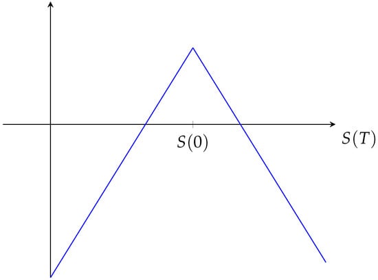
Figure 1. Profit function of a pure short straddle without securing long positions at the money. S denotes the S&P500 index value. The profit/loss (above/below the horizontal axis) depends on the final value $S\left(T\right)$ of the S&P500 at time T.

In a concretely traded Lambda strategy, several measurements for risk management are usually included. So, for example, in some variants, long positions in put- and/or call-options are opened to limit losses, or one could react to changing market environments by trading the underlying asset (or futures on the underlying), or close the open straddle positions if a certain threshold for losses or gains is reached. These variants will not be followed in this paper. Nevertheless, in the following, as well as the basic structure and parameters of the strategy, we also provide more details on these variants (which should be kept in mind for further research):

-

We choose a fixed time period of length T (e.g., two months, one month, one week, two trading days, …). For our simplified setting, we exclusively consider options with a remaining lifetime of one week.

-

For a given day t, we trade SPX options with remaining time to expiration T (or with the shortest possible time to expiration larger than or equal to T). We always initiate the trade at the closing time of the trading day t.

-

We always go short on the same quantity of call- and put-options with the same time to expiration (approximately) T and strike $K_1$ as close at-the-money as possible (i.e., with a strike as close as possible to the current value of the S&P500).

-

In the basic variant, we hold the option contracts until expiration.

-

Possible variant: In the case in which we aim to limit losses, we go long on the same quantity of put options with the same expiration and with a strike $K_2<K_1$, and/or we go long on the same quantity of call options with the same expiration and with a strike $K_3>K_1$. The strikes $K_2$ and/or $K_3$ of the long positions are chosen on the basis of various parameters (depending on what variant we are looking at). They will always depend on the current value of the S&P500 (at the trading date); in some cases they will also depend on the value of the S&P500-volatility index VIX or on a certain historical volatility, while, in other cases, they will depend on the prices of the put and/or call options in question.

-

Thus, upon entering the trade, we receive a positive premium of M USD, which is given by the price of the short positions (minus the price of the possible long positions).

-

Our reference currency in all cases is the U.S. dollar (USD).

-

For training our machine learning models, we always trade exactly one contract of options. In reality, when executing these trades, one would decide on the number of options to be traded by determining the required margin and calculate the possible number of contracts with the available capital.

-

Possible variant: Some variants of the strategy are equipped with an exit strategy, which means that all contracts are closed as soon as the losses/or gains from the call and put positions (since the last trading day) exceed a certain pre-defined level.

In the strongly simplified approach that we present in this paper, we ignore the possibility of buying long positions at strikes $K_2$ and $K_3$ and only sell the options at $K_1$. Moreover, we do not consider any exit strategy, but always hold the contracts until expiry. Our machine learning decision process now tries to decide, for a given trading day (and with respect to given market data), if the strategy should be executed or not. We assume that the decision is made at market close time on a daily basis.

2.2. Data

In our approaches to the machine learning problem, we focus on the following available data:

• daily historical put- and call-option price data1, which, amongst others, includes:

  -

  last ask and bid prices for any available strikes and expiry date

  -

  open, close, high and low prices per day

  -

  traded volume and open interest

• daily publicly available market data, such as

  -

  close, open, high and low of the underlying

  -

  close, open, high and low of the S&P500 volatility index VIX

  -

  USD-Libor rates

The historical option price data would also be available to us for earlier periods; however, starting from November 2011, the frequency of offered option expiration dates increased (essentially because of the introduction of SPXW options).

The data is clearly structured and is available on a very consistent basis.

The experiments in this paper are, therefore, based on a set of 2398 daily data samples, gathered and pre-processed from historical data between November 2011 and August 2022. Due to the consistency and quality of the available data, hardly any imputation was necessary on our side. Where required (i.e., almost exclusively in cases for USD-Libor rates), forward filling was used to make up for missing data points.

2.3. Evaluation Criteria

To evaluate the suitability of our trained model in relation to the problem, and to compare different models, a quality measure is needed. Since we are looking at a classification task, the usual metrics for classifiers are an obvious choice. However, even if our classifier were “really good” in terms of classifier metrics, it could still be “very bad”, in terms of profit made, if the classifier misses the most important choices (i.e., when the classifier invests in big losses, or does not invest in big gains). Thus, we also considered a second type of metric, all the members of which are connected to a profit measure.

2.3.1. Classification Metrics

For each of our validation and test sets, we automatically evaluate the usual classification metrics below. We used implementations from the Python-packages “scikit-learn” and “scipy.stats” and, therefore, follow their documentation (SciKit 2022, Scipy 2022) for the definitions.

-

accuracy: computes the accuracy (default is fraction) of correct predictions

-

recall: recall describes the quality of a classifier in finding all positive samples and is given by the ratio

$$\frac{tp}{tp+fn}$$

where $tp$ are the true positives and $fn$ are the false negatives

-

balanced accuracy: gives the accuracy of a classifier, adjusted by the probability of the outcome of each class. More precisely, it is defined as the average recall obtained for each class.

-

precision: describes the ability of the classifier to avoid false positives ($fp$) and is calculated by the ratio

$$\frac{tp}{tp+fp}$$

-

average precision: precision and recall are two measures which cannot be improved without worsening the other; it is always necessary to make trade-offs in the optimization of these two metrics. For this reason, the precision-recall curve is a very interesting visualization. The average precision metric provides a summary of the precision-recall curve in one single metric as the weighted mean of precisions at given thresholds $P_n$, where the weights are given by the increase in the recall metric from the previous threshold $(R_n-R_{n-1})$:

$$AP=\sum _n(R_n-R_{n-1})P_n$$

-

negative average precision: the same as average precision above, but with both inverted targets and inverted predictions as parameters.

-

average fraction of positives (i.e., average fraction of trades): is calculated by taking the mean of all ${\widehat{y}}_i$, which gives the number of executed trades as a fraction.

-

PRC: the precision recall curve gives the precision-recall pairs for varying thresholds.

-

PRC (auc): collects information of the PRC in one metric by calculating the area under the curve.

-

F1 score: again a combined measure of precision and recall, which can be interpreted as the harmonic mean of these two metrics.

$$F1=2\ast \frac{recall·precision}{recall+precision}$$

-

Brier score loss: measures the mean squared difference between the predicted probability and the actual outcome

-

cross-entropy loss (or negative log loss): the loss function used in logistic regression for a classifier which gives a prediction probability $\widehat{y}$ to an actual outcome y. In the binary case (with $y\in \{0,1\}$ and p the probability of $y=1$), this leads to:

$$L_{log}(y,p)=-(ylogp+(1-y)log(1-p))$$

-

ROC curve: the ROC (receiver operating characteristic) curve is determined by plotting the fraction of true positives to the fraction of false positives for the varying threshold.

-

ROC (auc): collects information on the ROC curve in one metric by calculating the area under the curve.

-

Pearson correlation coefficient: a measure of the linear relationship between two datasets. It tests the null hypothesis that the distributions of the sets are uncorrelated and normally distributed.

-

Spearman correlation coefficient: measures the monotonicity of the relationship between two datasets. It is non-parametric and, in contrast to the Pearson correlation, does not assume both datasets to be normally distributed. As with other correlation coefficients, the Pearson and Spearman coefficients have values between −1 and +1 where 0 means no correlation.

-

Pearson/Spearman correlation coefficient p-value: represents the approximate probability that an uncorrelated system will produce datasets that have a Pearson/Spearman correlation at least as extreme as the one computed from these datasets.

2.3.2. Profit Metrics

The second class of metrics that we are interested in are metrics corresponding to profit calculations. First, we allow all the above “standard” classification metrics to be weighted with respect to the corresponding profit made. This means that, for a given sample y and a given prediction of our model $\widehat{y}$, we weight the above metrics with respect to the profit (or loss) one would have achieved with this specific trade. This implies that trades with big gains or losses are weighted more than trades with minimal gains or losses. Additionally, we calculate the following metrics:

-

total profit: for given predictions ${\widehat{y}}_i\in \{0=\mathrm{do}\mathrm{not}\mathrm{trade},1=\mathrm{trade}\}$ and given profits $p_i$, we calculate the total profit by simply calculating the sum:

$$\mathrm{total}\mathrm{profit}=\sum _{i=1}^n{\widehat{y}}_i{p}_i$$

-

long-and-short total profit: essentially the same as the total profit above, but instead of 0 (do not trade), we use −1, therefore shorting the strategy in those cases instead of not trading at all.

-

average profit: is determined by taking the mean in an analogous way to the total profit above:

$$\mathrm{average}\mathrm{profit}=\frac{1}{n}\sum _{i=1}^n{\widehat{y}}_i{p}_i$$

-

average profit per trade: is determined by taking the mean as above, but only where ${\widehat{y}}_i$ is not 0.

-

standard deviation of profit per trade: is determined by taking the standard deviation of the profits where ${\widehat{y}}_i$ is not 0.

-

downside deviation of profit per trade: is determined by taking the standard deviation of the profits where ${\widehat{y}}_i$ is not 0 and $p_i<0$.

-

maximum drawdown: maximum loss from a peak to a subsequent trough before a new peak is reached in the timeline of the cumulated profits, i.e.,:

$$\mathrm{maximum}\mathrm{drawdown}=\underset{1\le n_1\le n_2\le n}{min}\sum _{i=n_1}^{n_2}{\widehat{y}}_i{p}_i$$

-

Sharpe ratio: the ratio between the average excess return of the predicted strategy executions over a risk-free asset and its standard deviation. As a risk free asset, we use the six-month USD Libor. For computing the return of each strategy execution, we assume a margin of USD 100,000 to be deposited at the quote date of each short straddle and that each strategy portfolio consists of one contract (100 pieces) call- and one contract put-option. The return for a given prediction y and given profit p is then:

$$\mathrm{strategy}\mathrm{execution}\mathrm{return}=\frac{100·y·p}{100000}=\frac{y·p}{1000}$$

-

Sortino ratio: very similar to the Sharpe ratio above, but using the downside deviation instead of the standard deviation that is used for the Sharpe ratio.

Since it is naturally our goal for our models to be able particularly to predict the correct outcome for trades which lead to big gains or losses, we focus on metrics which take the profit into account.

2.4. Features

For a given trading day on which we consider the execution of the strategy, we use the following features:

-

put price: we use the average of the last bid and ask price and reduce it by USD 0.1 for our sell price

-

call price: is determined analogously to the put price

-

strike: current strike price, which is the closest strike price to the current S&P500 value

-

days to expiry: the number of days to expiration of the options

-

S&P500 close of last 20 trading days: the absolute closing price of the S&P500

-

S&P500 close of last 20 trading days relative to the S&P500 value on the previous day

-

S&P500 high: the highest value of the S&P500 on the current day

-

S&P500 low: the lowest value of the S&P500 on the current day

-

VIX close of trading day and the previous 20 trading days

-

VIX high: the highest value of the VIX on the current day

-

VIX low: the lowest value of the VIX on the current day

-

1-month USD Libor: the current value of the one-month US-Dollar London Inter-Bank Offered Rate

-

six-month USD Libor: the current value of the six-month US-Dollar London Inter-Bank Offered Rate

-

pm-settled: indicates whether, for the settlement of the currently considered options, the closing (pm-settled) or the opening value of the S&P500 is relevant (i.e., whether the option is of SPXW-type or of SPX-type)

Note that, we consider data from the last 20 days before each trading date, since we work with options with a remaining lifetime of, at most, one week. It seems extremely unlikely that data older than one month would have any influence on this type of short-time strategy.

2.5. Modeling

We used model implementations of the Sklearn Python library for our experiments. In the following, we briefly describe the evaluated models, while closely following the descriptions found in the SciKit-Learn documentation SciKit (2022).

2.5.1. Decision Trees

We use three different models based on decision trees:

-

A bare decision tree classifier relying on an instance of a simple classical decision tree.

-

The random forest classifier is an averaging algorithm based on randomized decision trees. It is a perturb-and-combine technique specifically designed for trees. In this sense, a diverse set of classifiers is created by introducing randomness in the classifier construction. The prediction of the ensemble is given as the averaged prediction of the individual classifiers. Each tree in the ensemble is built from a sample drawn with replacement from the training set. Furthermore, when splitting each node during the construction of a tree, the best split, in our case, is determined from all the input features. These two sources of randomness are introduced to decrease the variance of the forest estimator. The scikit-learn implementation combines classifiers by averaging their probabilistic prediction instead of letting each classifier vote for a single class.

-

The extremely randomized trees classifier (extra_trees) is very similar to the random forest classifier and also represents an averaging algorithm based on randomized decision trees. The main difference is that, instead of looking for the most discriminative thresholds, multiple thresholds are drawn randomly for each possible feature and the best of these randomly generated thresholds is chosen as the splitting rule.

2.5.2. Logistic Regression with SGD Training

Logistic regression is a linear model, where the probabilities describing the possible outcomes of a single trial are modeled using a logistic function. In our experiments, we apply logistic regression with stochastic gradient descent learning; hence, the corresponding results in the sections below are also presented under the name “SGD”.

For instance, binary class $l_2$ penalized logistic regression represents an optimization problem that minimizes the following cost function:

$$\underset{w,c}{min}\frac{1}{2}{w}^{T}w+C\sum _{i=1}^{n}log(exp(-y_i(X_i^{T}w+c))+1).$$

where w are the parameters, $X_i$ the features, $y_i$ the targets and C is the regularization parameter.

2.5.3. k Nearest Neighbors (kNN) Classifier

Neighbors-based classification is a type of instance-based learning or non-generalizing learning: it does not attempt to construct a general internal model, but simply stores instances of the training data. Classification is computed from a simple majority vote of the nearest neighbors of each point: a query point is assigned the data class which has the most representatives within the nearest neighbors of the point.

The type of classifier we use is based on the k nearest neighbors of each query point, where k is an integer value.

For the distance metric for the tree there are two different possible configurations: Euclidian and cosine.

Two different possible weight functions for prediction are available:

-

Uniform: All points in each neighborhood are weighted equally.

-

Distance: Points are weighted by the inverse of their distance. In this case, closer neighbors of a query point will have a greater influence than neighbors which are further away.

2.5.4. Multi-Layer Perceptron Classifier

A multi-layer perceptron (MLP) learns a function $f(·):{\mathcal{R}}^m\to {\mathcal{R}}^o$ by training on a dataset, where m is the number of dimensions for input and o is the number of dimensions for output—which is 1 in our case. Given a set of features $X=x_1,x_2,\dots ,x_m$ and a target y, it can learn a non-linear function approximator for classification. It is different from logistic regression, in that, between the input and the output layer, there can be one or more non-linear layers, called hidden layers. The structure of an MLP with one hidden layer is depicted in Figure 2.

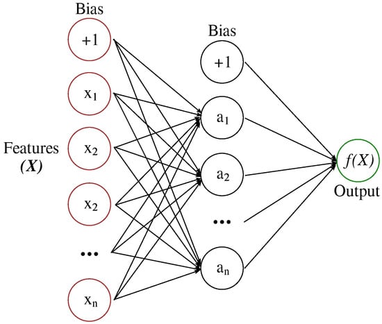
Figure 2. Multilayer perceptron (MLP) with one hidden layer.

2.5.5. AdaBoost Classifier

The core principle of AdaBoost is to fit a sequence of weak learners (i.e., models that are only slightly better than random guessing, such as small decision trees) on repeatedly modified versions of the data. The predictions from all of them are then combined through a weighted majority vote (or sum) to produce the final prediction. The data modifications at each so-called boosting iteration consist of applying weights $w_1,w_2,\dots w_N$ to each of the training samples. Initially, these weights are all set to $w_i=1/N$, so that the first step simply trains a weak learner on the original data. For each successive iteration, the sample weights are individually modified and the learning algorithm is reapplied to the re-weighted data. At a given step, the training examples that were incorrectly predicted by the boosted model induced at the previous step have their weights increased, whereas the weights are decreased for those that were predicted correctly. As iterations proceed, examples that are difficult to predict receive ever-increasing influence. Each subsequent weak learner is, thereby, forced to concentrate on the examples that are missed by the previous learners in the sequence.

2.5.6. Gradient-Boosting Classifier

Gradient tree boosting (GB) is a generalization of boosting to arbitrary differentiable loss functions. It builds an additive model in a forward stage-wise fashion; it allows for the optimization of arbitrary differentiable loss functions. In each stage n_classes_, regression trees are fit on the negative gradient of the binomial or multinomial deviance loss function. Binary classification, as we use it, is a special case, where only a single regression tree is induced.

2.5.7. C-Support Vector Classification

Given a set of training examples, each marked as belonging to one of two categories, a support-vector machine (SVM) training algorithm builds a model that assigns new examples to one category or the other, making it a non-probabilistic binary linear classifier. SVM maps training examples to points in space so as to maximise the width of the gap between the two categories. New examples are then mapped into that same space and are predicted to belong to a category based on which side of the gap they fall.

The Sklearn implementation we use (libsvm_svc) accepts a set of different kernel types to be used in the algorithm, such as the RBF kernel with the function $exp(-\gamma \parallel x-x^{\prime }{\parallel }^2)$.

2.5.8. Other Classifiers

In addition to the self-contained models listed above, we also include three more types of classifiers for reference:

-

ensemble: represents a combination of the other classifiers that tries to improve generalizability or robustness over a single estimator. It is determined in the course of the hyperparameter search.

-

Strat: randomly samples one-hot vectors from a multinomial distribution parametrized by the empirical class prior probabilities.

-

All: a “dummy classifier” that represents the trade-always strategy for comparison.

2.5.9. Hyperparameters

Hyperparameters, as well as pre-processing pipelines, were optimized for each classifier using Autosklearn (see Aut 2022, Feurer et al. 2015, 2020). Pre-processing methods include, among others, the methods fast ICA and PCA. A hold-out split with 33% validation samples was chosen, optimized for validation of the average-precision via a Bayesian optimizer (Autosklearn for this purpose extends the Bayesian optimization package SMAC3, see Lindauer et al. (2021), to allow for asynchronous parallel optimization). The optimization time was set to one hour with 40 cores, 10 min per run and an ensemble size of 25. Each final model was comprised of 25 sub-models, each with its own pre-processing and individual hyperparameters being of the same model class. This strategy was chosen because it has been shown empirically that ensembles outperform single models (see e.g., Lacoste et al. (2014)).

Models are weighted by their performance in the validation set.

The exact hyperparameter and ensemble configurations are omitted here due to their extensiveness, but are available upon request. The configuration space for each algorithm can be found here2.

2.6. Experiments

For all our experiments, we chose a prequential evaluation approach, as such an approach is very useful for streaming data (e.g., see Gama et al. (2013)). This means, for given data in a time span $[0,T]$, we split the whole time span into sub-intervals of a given duration $\Delta t$ (during our research, we found that working with one-month splits yielded the best training results). Thus, we have $t_i$ in our time span $\{t_0=0,t_1,t_2,\dots ,t_n=T\}$, such that $t_i-t_{i-1}=\Delta t$.

For a fixed point $t_i$ with $0<i<(n-1)$, we now split our data into three separate sets as illustrated in Figure 3. The data available in the time span $[0,t_i]$ are the training set for this iteration, $(t_i,t_{i+1}]$ are the validation set and $(t_{i+1},t_{i+2}]$ are the test set for our machine learning models. This means that we train our data on all the data available up to $t_i$ and use the next intervals in time for validation and testing, respectively. In the next iteration, the training set is extended until $t_{i+1}$ and validation and testing is executed on the subsequent sets, and so forth.

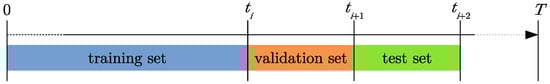
Figure 3. Prequential evaluation scheme.

After each iteration, a classification threshold optimization is performed. That is, the algorithm determines above which exact threshold (in steps of 0.1) of the probability given by the model’s predictions on the validation set trading should be performed to yield the highest possible average profit.

Thus, we finally obtain a series of metrics on test sets, which are streaming over time intervals $(t_i,t_{i+1}]$. Based on these, we can either examine the behaviour of the metrics over time, or we can calculate statistics (e.g., mean or standard deviations) over a range of such test sets. The exact parameters of the executed experiments are listed below.

Experiment Parameters

-

Feature columns: we use all features listed in Section 2.5 above.

-

Prequential split frequency: 1 month

-

Start date for test sets: Jan 2017

-

Start date of training set: 2011

For our final evaluation runs, we also added the validation data to the test sets to increase the number of samples and improve the training results. We executed this setup for all our machine learning algorithms in three model variants each; that is, by starting the execution with different seeds in each rerun, we obtained varying results that allowed us to further investigate the volatility of the models.

2.7. Result Overview

On the following pages, we illustrate and discuss only a small selection of the obtained results, based on some exemplary models. For comparison, we added the simple “trade always” strategy, which is denoted by “All” in the tables and the visualizations.

It should be emphasized that the trading period from January 2017 until August 2022 contained very challenging periods, especially at the end of the trading year 2018, during the first wave of the coronavirus crisis in spring 2020, and in the period from January 2022 until August 2022 (i.e., the war in the Ukraine and the resulting economic dislocations). In these periods, we, for example, had to face temporary extreme drawdowns and sometimes very high volatility. For a visualisation of the situation, see the charts of the S&P500 and of the VIX from January 2017 until August 2022 in Figure 4 and Figure 5 below.

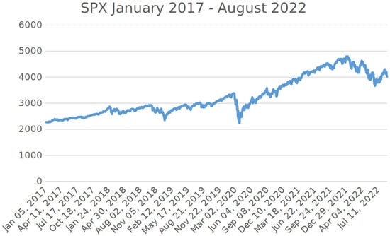
Figure 4. Chart of the S&P500 from January 2017 until August 2022.

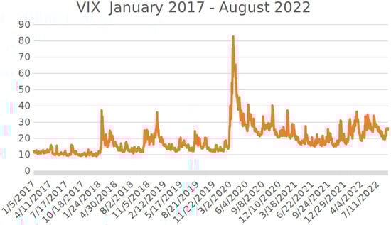
Figure 5. Chart of the VIX from January 2017 until August 2022.

We start with plots (see Figure 6, Figure 7, Figure 8 and Figure 9) showing the timelines of the cumulative profits of selected models and their variants. The blue lines in each plot represent the cumulative profits of the model variants when deciding between either trading or not trading at all, while the red lines show the behaviour when, instead of not trading, the strategy is even being shorted (i.e., buying two option contracts instead of selling them). The black line denotes the trade-always strategy (“All”), while the grey area represents a multitude of stratified (randomly chosen decisions) paths (“Strat”).

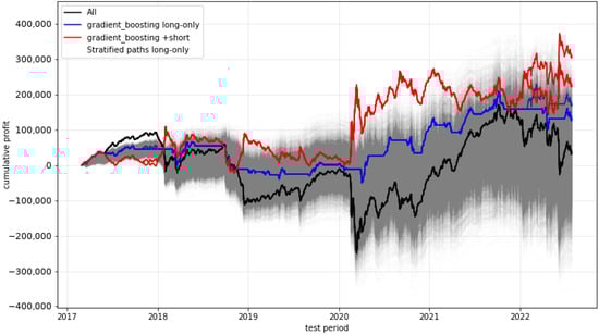
Figure 6. Cumulative profit of the gradient-boosting predictions. The black line shows the trade-always strategy (“All”), while the grey area represents a multitude of stratified paths (“Strat”). Multiple lines of the same color (i.e., blue and red) denote different model variants (or seeds).

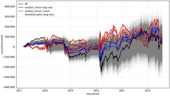
Figure 7. Cumulative profit of the random forest predictions.

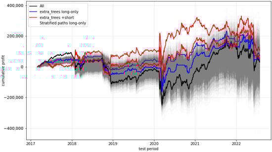
Figure 8. Cumulative profit of the extra trees predictions.

Figure 9. Cumulative profit of the ensemble predictions.

The most promising development is provided by the gradient-boosting approach. (All other approaches, including the approaches not visualised here, do not provide obvious significant outperformance of any form.) The main advantage of the gradient-boosting algorithm seems to be that, in literally all (three) critical phases during the test period, a non-trading strategy was followed. So, it seems that this approach effectively anticipated situations which were extremely disadvantageous for trading the short straddle. This was especially evident in the phase of the first coronavirus wave in spring 2020, when severe losses had strongly weakened the profits of the “All” strategy and also of the profits for all other approaches.

This impression is additionally supported when considering the variant of the strategy where, instead of non-trading, the strategy is shorted (red line). This approach results in high gains during the critical phases.

It could be argued that a permanent non-trading strategy conducted in a perfect way would avoid losses in all critical phases. However, such a non-trading strategy would not provide any gains, whereas the gradient-boosting approach provides significant positive profits.

Altogether, the development path of the profits shows a quite low-volatile form.

It is of interest that, if we consider the single metrics for the different approaches in more detail, then the “obvious superiority“ of the gradient-boosting approach over the other approaches (and the “All“ strategy) is not reflected so clearly. This can be seen in the following examples in which we analyze which models exhibit a statistically significant outperformance compared to the trade-always (“All”) strategy with respect to certain metrics (the integer in brackets next to the model name in the table represents the seed of the best-performing model variant).

We conclude that, in the case of maximal drawdown, the gradient-boosting approach shows a clear and significant dominance over all other approaches.

For the interested reader, as additional information on the performance of the different approaches, detailed metrics and their interpretations can be found in Appendix A; boxplots on the total profit per test set, on the average precision over all test sets, and on the balanced accuracy over all test sets can be found in Appendix B.

We return to our favorite approach, the gradient-boosting approach and we consider all the metrics for this approach compared with the metrics of the “All“-trading approach Table 1.

Table 1. Mean and standard deviation of the metrics on the test sets for gradient boosting (seed = 42) and the trade-always strategy.

	Gradient_Boosting		All
	Mean	std	Mean	std
accuracy	0.49536	0.18367	0.58386	0.16314
balanced_accuracy	0.50000	0.00000	0.50000	0.00000
average_precision	0.58386	0.16314	0.58386	0.16314
neg_average_precision	0.41614	0.16314	0.41614	0.16314
neg_brier_score	0.34217	0.14704	0.41614	0.16314
f1	0.32455	0.37499	0.72386	0.13355
neg_log_loss	1.42258	1.47060	14.37345	5.63480
precision	0.26268	0.31561	0.58386	0.16314
recall	0.44615	0.50096	1.00000	0.00000
roc_auc	0.50000	0.00000	0.50000	0.00000
prc_auc	0.20807	0.08157	0.20807	0.08157
accuracy_weighted	0.50053	0.22299	0.56093	0.21437
balanced_accuracy_weighted	0.50000	0.00000	0.50000	0.00000
average_precision_weighted	0.56093	0.21437	0.56093	0.21437
neg_average_precision_weighted	0.43907	0.21437	0.43907	0.21437
neg_brier_score_weighted	0.34062	0.16345	0.43907	0.21437
f1_weighted	0.31416	0.36962	0.69437	0.18283
neg_log_loss_weighted	1.40911	1.50248	15.16521	7.40419
precision_weighted	0.25381	0.31599	0.56093	0.21437
recall_weighted	0.44615	0.50096	1.00000	0.00000
roc_auc_weighted	0.50000	0.00000	0.50000	0.00000
prc_auc_weighted	0.20807	0.08157	0.20807	0.08157
avg_profit_weighted	100	891	28	1472
tot_profit_weighted	2029	19,154	569	30,599
losh_tot_profit_weighted	3489	30,402	569	30,599
avg_trading_profit_weighted	224	1336	28	1472
std_trading_profit_weighted	3323	2098	4047	3218
downt_std_trading_profit_weighted	1958	1686	2672	2553
mdd_weighted	8759	15,607	25,375	29,953
avg_trades_weighted	0.44615	0.50096	1.00000	0.00000
avg_profit_norm_weighted	0.00000	0.00000	−0.00000	0.00000
tot_profit_norm_weighted	0.00000	0.00000	0.00000	0.00000
avg_trading_profit_norm_weighted	0.00000	0.00000	−0.00000	0.00000
sharpe	0.364		−0.006
sortino	0.317		−0.006

We wish to highlight that, in Table 1, all the metrics, with the exception of the Sharpe ratio and the Sortino ratio, were calculated in the following way: We divided the whole trading period into trading periods of one month and took the mean and the standard deviation of the resulting metric values. The Sharpe ratio and the Sortino ratio, however, were calculated from the profits over the whole trading period. We used the values of the six-month USD Libor as reference interest rate values and assumed, for each single trade, an investment base of USD 100.000.

In Figure 10, we illustrate the trade/non-trade decisions in the gradient-boosting approach, parallel to the development of the S&P500-index over the whole trading period.

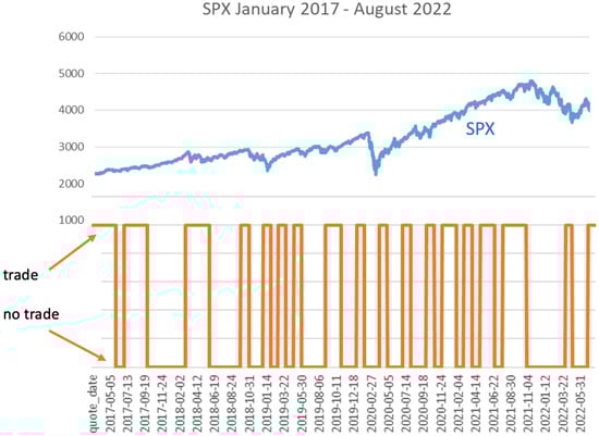
Figure 10. Trading decisions (orange line) for the gradient-boosting approach.

If the orange line is on the higher level, then, at these times, trading is indicated. It can be seen that there is not a strong fluctuation, but that there are longer periods of trading or of non-trading. The “decision-output“ is not a 1 (=trade) or a 0 (=no-trade) indication, but we obtain probabilities on whether a trade seems to become successful or not. This means that we obtain probabilities p between 0 and 1; we trade if p is larger or equal to $0.5$ and we do not trade if p is less than $0.5$. The concrete probabilities are shown in Figure 11.

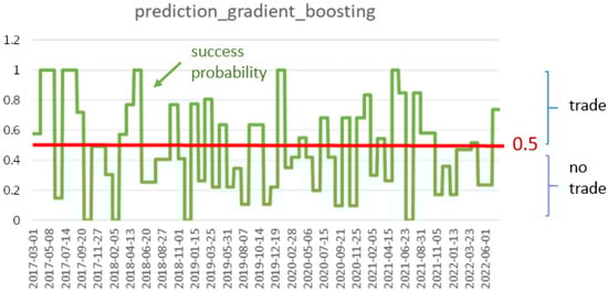
Figure 11. Trading probabilities (green line) for the gradient-boosting approach.

In Figure 12, we illustrate the distribution of profits per trade of the “All-strategy” (blue) and of the “gradient-boosting strategy” (orange). Again, it can be seen that the gradient-boosting approach avoids the really large losses.

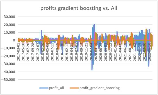
Figure 12. Distribution of profits for the “All-strategy” (blue) and for the “gradient-boosting strategy” (orange).

It would be tempting to work directly with the probabilities p, implying the more option-contracts are traded, the higher the probability p. However, when considering profits weighted by the probabilities p instead of the decision-parameters 0 and 1, it is found that this would not result in an improvement.

3. Conclusions and Next Steps for Further Research

In this study, we have built the basic environment for an extensive investigation of the application of machine learning approaches to decision-finding for certain option-trading strategies (“Lambda-strategies”). To do so, we focused on an analysis of a simple trade-/non-trade-decision problem for short-straddles. We emphasize that our test period, apart from a very calm period from 2012 until 2017, included the very recent, very challenging time period from January 2020 until August 2022 (e.g., coronavirus waves, the Ukraine war, energy crises) with sharp drawdowns and, occasionally, extremely high volatility. Given this, the main, and rather encouraging, result is that, at least for this basic decision problem, the application of a gradient-tree-boosting approach can significantly improve (including in very challenging financial markets) the success of trading decisions; this is in direct contrast to existing findings, as presented, for example, in Tino et al. (2001). To the best of our knowledge, these are the first advances in applying machine learning methods to the broad field of sophisticated option-trading strategies, as current available studies have focused on the prediction of prices, volatility or more basic derivatives. In light of our findings, we intend, in future, to concentrate on the optimal use of gradient-boosting for an extended analysis of the Lambda strategy with all its variants.

As was pointed out in the description of the variants of the Lambda strategy, in the next step, we will define and analyse a decision problem to decide which of the following variants of the strategy we should execute:

-

$V_0$: trading naked short positions at $K_1$ and hold until expiration

-

$V_1$: trading naked short positions and close if a certain loss or gain threshold is reached (losses/gains with respect to the opening of the positions)

-

$V_2$: trading short positions at $K_1$ and, additionally, a long put position at a certain predefined strike $K_2$

-

$V_3$: trading short positions at $K_1$ and, additionally, a long call at a certain predefined strike $K_3$

-

$V_4$: trading short positions at $K_1$ and, additionally, long positions at $K_2$ and $K_3$, respectively

-

$V_5$: trading short positions at $K_1$ and use futures to cover for losses when a certain underlying threshold is reached

-

$V_6$: do not trade at all

Another very interesting topic for future research would be based directly on investigations reported in our preceding paper about the deviations between implied volatility found in S&P500 option markets and the manifest volatility. Instead of directly training the model on executing the Lambda strategy, we could train models to estimate the subsequently realized volatility (see for example Osterrieder et al. (2020) or Carr et al. (2020)) and trade based on such estimates on future differences to the current implied volatility in the options market. One advantage of this approach would be the possibility to build upon existing research in the estimation of volatility via machine learning models.

There are also many possibilities on the technical side that can be explored. For example, we have not reached the limits in terms of the algorithms that can be used and believe that the application of more complex and modern methods to our defined problem could yield further insights. In this regard, we view Hopfield networks (cf. Ramsauer et al. (2020)) as potentially valuable candidates.

References

- Auto-Sklearn Documentation. 2022. Available online: https://automl.github.io/auto-sklearn/master/ (accessed on 3 September 2022).
- Babenko, Vitalina, Andriy Panchyshyn, L. Zomchak, M. Nehrey, Z. Artym-Drohomyretska, and Taras Lahotskyi. 2021. Classical machine learning methods in economics research: Macro and micro level example. WSEAS Transactions on Business and Economics 18: 209–17. [Google Scholar] [CrossRef]
- Bourke, Daniel. 2020a. A 6 Step Field Guide for Building Machine Learning Projects. Available online: https://towardsdatascience.com/a-6-step-field-guide-for-building-machine-learning-projects-6e4554f6e3a1 (accessed on 30 March 2022).
- Bourke, Daniel. 2020b. A 6 Step Framework for Approaching Machine Learning Projects. Available online: https://github.com/mrdbourke/zero-to-mastery-ml/blob/master/section-1-getting-ready-for-machine-learning/a-6-step-framework-for-approaching-machine-learning-projects.md (accessed on 30 March 2022).
- Brunhuemer, Alexander, Gerhard Larcher, and Lukas Larcher. 2021. Analysis of option trading strategies based on the relation of implied and realized S&P500 volatilities. ACRN Journal of Finance and Risk Perspectives, Special Issue 18th FRAP Conference 10: 106–203. [Google Scholar]
- Carr, Peter, Liuren Wu, and Zhibai Zhang. 2020. Using machine learning to predict realized variance. Journal of Investment Management 18: 1–16. [Google Scholar]
- Chiang, Thomas C. 2020. Risk and policy uncertainty on stock-bond return correlations: Evidence from the us markets. Risks 8: 58. [Google Scholar] [CrossRef]
- Cohen, Gil. 2022. Algorithmic trading and financial forecasting using advanced artificial intelligence methodologies. Mathematics 10: 3302. [Google Scholar] [CrossRef]
- Day, Theodore E., and Craig M. Lewis. 1997. Initial margin policy and stochastic volatility in the crude oil futures market. The Review of Financial Studies 10: 303–32. [Google Scholar] [CrossRef]
- Del Chicca, Lucia, and Gerhard Larcher. 2012. A comparison of different families of put-write option strategies. ACRN Journal of Finance and Risk Perspectives 1: 1–14. [Google Scholar]
- Feurer, Matthias, Katharina Eggensperger, Stefan Falkner, Marius Lindauer, and Frank Hutter. 2020. Auto-sklearn 2.0: Hands-free automl via meta-learning. arXiv arXiv:2007.04074. [Google Scholar]
- Feurer, Matthias, Aaron Klein, Katharina Eggensperger, Jost Springenberg, Manuel Blum, and Frank Hutter. 2015. Efficient and robust automated machine learning. Advances in Neural Information Processing Systems 28: 2962–970. [Google Scholar]
- Gama, João, Raquel Sebastião, and Pedro Pereira Rodrigues. 2013. On evaluating stream learning algorithms. Machine Learning 90: 317–46. [Google Scholar] [CrossRef]
- Lacoste, Alexandre, Mario Marchand, François Laviolette, and Hugo Larochelle. 2014. Agnostic bayesian learning of ensembles. Papar presented at International Conference on Machine Learning (PMLR), Bejing, China, June 22–24; pp. 611–19. [Google Scholar]
- Larcher, Gerhard, Lucia Del Chicca, and Michaela Szölgyenyi. 2013. Modeling and performance of certain put-write strategies. The Journal of Alternative Investments 15: 74–86. [Google Scholar] [CrossRef]
- Lindauer, Marius, Katharina Eggensperger, Matthias Feurer, André Biedenkapp, Difan Deng, Carolin Benjamins, Tim Ruhopf, René Sass, and Frank Hutter. 2021. Smac3: A versatile bayesian optimization package for hyperparameter optimization. Journal of Machine Learning Research 23: 54–54. [Google Scholar] [CrossRef]
- Nagula, Pavan Kumar, and Christos Alexakis. 2022. A new hybrid machine learning model for predicting the bitcoin (BTC-USD) price. Journal of Behavioral and Experimental Finance 36: 100741. [Google Scholar] [CrossRef]
- Oktoviany, Prilly, Robert Knobloch, and Ralf Korn. 2021. A machine learning-based price state prediction model for agricultural commodities using external factors. Decisions in Economics and Finance 44: 1063–85. [Google Scholar] [CrossRef]
- Osterrieder, Joerg, Daniel Kucharczyk, Silas Rudolf, and Daniel Wittwer. 2020. Neural networks and arbitrage in the VIX. Digital Finance 2: 97–115. [Google Scholar] [CrossRef]
- Ramsauer, Hubert, Bernhard Schäfl, Johannes Lehner, Philipp Seidl, Michael Widrich, Thomas Adler, Lukas Gruber, Markus Holzleitner, Milena Pavlović, Geir Kjetil Sandve, and et al. 2020. Hopfield networks is all you need. arXiv arXiv:2008.02217. [Google Scholar]
- Santa-Clara, Pedro, and Alessio Saretto. 2009. Option strategies: Good deals and margin calls. Journal of Financial Markets 12: 391–417. [Google Scholar] [CrossRef]
- SciKit-Learn Documentation. 2022. Available online: https://scikit-learn.org/stable/ (accessed on 25 August 2022).
- Scipy-Stats Documentation. 2022. Available online: https://docs.scipy.org/doc/scipy/reference/stats.html (accessed on 3 September 2022).
- Sheng, Yankai, and Ding Ma. 2022. Stock index spot-futures arbitrage prediction using machine learning models. Entropy 24: 1462. [Google Scholar] [CrossRef]
- Tino, Peter, Christian Schittenkopf, and Georg Dorffner. 2001. Financial volatility trading using recurrent neural networks. IEEE Transactions on Neural Networks 12: 865–74. [Google Scholar] [CrossRef]
- Ungar, Jason, and Matthew T. Moran. 2009. The cash-secured put-write strategy and performance of related benchmark indexes. The Journal of Alternative Investments 11: 43–56. [Google Scholar] [CrossRef]
- Wen, Wen, Yuyu Yuan, and Jincui Yang. 2021. Reinforcement learning for options trading. Applied Sciences 11: 11208. [Google Scholar] [CrossRef]
- Wiese, Magnus, Robert Knobloch, Ralf Korn, and Peter Kretschmer. 2020. Quant GANs: Deep generation of financial time series. Quantitative Finance 20: 1419–440. [Google Scholar] [CrossRef]
Publisher’s Note: MDPI stays neutral with regard to jurisdictional claims in published maps and institutional affiliations. |
© 2022 by the authors. Licensee MDPI, Basel, Switzerland. This article is an open access article distributed under the terms and conditions of the Creative Commons Attribution (CC BY) license (https://creativecommons.org/licenses/by/4.0/).