Abstract
A cost effective, fast, and accurate technique was needed to measure the vapor composition of a binary system (ethanol-water) and also that of a liquid composition in a ternary system (acetic acid-acetol–water) in a microbubble distillation unit. Cheap TGS-series gas sensors were used for this purpose with both calibrations and measurements carried out in a specially designed chamber. A single parameter polynomial regression was fitted to the binary system, and a two parameter polynomial with an interaction term was fitted to the ternary system. The correlation coefficient, R-squared, was found to be greater than 0.99 for both systems, thus validating the implementation of this novel sensor.
1. Introduction
Gas sensors are used to detect the presence of gas contaminants in the environment of interest. The detection principle involves measuring changes in the physical or chemical properties that occur on the sensing element due to the action of one or more of species of gas [1]. The goal of gas sensor experiments is to analyze information provided by stimulated sensors in order to qualify and/or quantify the targeted substances in the medium under study [2,3]. However, the analysis techniques and degree of accuracy required depend mainly on the proposed application of the gas sensors. As a result, the answer might involve a straightforward mathematical calculation or might necessitate an advanced level of analytical complexity [4,5].
Gas sensors offer an attractive solution for a wide range of applications in which gas sensing is an integral part of the system. Gas leakage detectors/alarms, air/food quality control, breath analyzers, pollutant monitoring, medical diagnostics, and electronic noses are common areas in which gas sensors have been applied [6,7,8,9,10,11].
Different technologies have been adapted in the manufacturing process of gas sensors in order to improve their characteristics and performance [12]. Among these, the method based on measuring the changes in the electrical properties of a sensing element built from a metal oxide semiconductor (MOX) offers many valuable advantages, such as high sensitivity, fast response and recovery times, low power consumption, long life, miniature size, availability, and low cost [13].
The MOX gas sensors used in the current work exhibited all of these benefits. Brief principles for the measurements will be introduced. Details of the experimental rig and the method of analysis will be described.
1.1. Metal Oxide Gas Sensors
The sensing element of the metal oxide gas sensors was made from semiconductor materials. Typically, tin-dioxide (SnO2) doped with a tiny quantity of catalytic material such as platinum or palladium was used to enhance sensitivity and/or selectivity. When the sensing material is heated up using a heater located in the gas sensor, electrons are lost by adsorbing oxygen from the surrounding air, causing an increase in the electrical resistance according to the reaction [13]
In the presence of a reducing gas species X (e.g., organic vapor), it will act to reduce the negative charge density by reacting with the adsorbed oxygen, returning the previously donated electrons back to the semiconductor crystal according to the reaction
As a result of this, the resistance of the sensing element will be decreased. The rate of the second reaction is affected by the concentration of the reducing gas, temperature, and working conditions.
The use of metal oxide (MOX) gas sensors under atmospheric conditions has been widely studied due to the low cost of their manufacture and ease of use. However, they generally exhibit low selectivity. For this reason there is no ideal gas sensor that can respond to one single component from a mixture of reducing gases. Many techniques have been developed to enhance the selectivity of gas sensors, either by modifying their design parameters or detection performance [14,15,16]. The current study involves the application of using responses from several sensors with different sensitivities to form a particular signature that represents a defined chemical mixture to the recently developed methodology of microbubble distillation. Microbubble distillation is inherently a transient process with potentially rapid kinetics creating a difficult challenge for the chemosensor system.
Figure 1 shows a simple circuit diagram used to drive a MQ-3 type gas sensor. This sensor has six pins: two A and two B pins that act as sensing element terminals and two H terminals for the heater to raise the temperature of the sensing element up to its working temperature. The change in conductivity can be detected by monitoring the voltage drop over the load resistor RL.
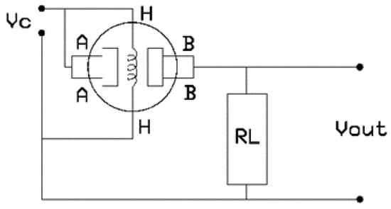
Figure 1.
Gas sensor driving circuit schematics.
1.2. Gas Sensor Array Models Based on Polynomial Regression
Although many techniques have been adapted for the purpose of identifying components using electronic noses, for this study it was found that polynomial regression provided a good fit to the relation between the responses of the gas sensor across the entire range of concentrations considered. Furthermore, the implementation of polynomial regression avoided the potential complexity that could have arisen from the use of other techniques, such as neural networks [4,5,17,18].
2. Materials and Methods
2.1. Microbubble Distillation Unit
Samples were taken from a running microbubble distillation unit. In the first set of experiments measurements of ethanol vapor concentration were made. The liquid composition for acetic acid–acetol–water liquid concentrations were obtained in a second set of experiments.
The microbubble distillation unit consisted of a rectangular tank with a microbubble diffuser, connected to a fluidic oscillator, comprising a microbubble generator [19]. Temperature-controlled air was passed through the diffuser. When the injected microbubbles rise through a thin layer of liquid mixture, they become enriched with the more volatile component within a very short contact time, on the order of a few milliseconds. This means that air leaving the system will contain a concentration of volatile liquid vapors that is greater than the equilibrium concentration. Furthermore, fluxes will be higher than those associated with traditional separation processes based on vapor-liquid equilibrium. Details of the separation process using microbubble-mediated distillation, modeling, and a description of the experimental rig can be found in [19,20]. It is the strongly nonlinear and transient response of microbubble distillers that requires sensitive gas sensors to infer system performance.
2.2. Materials and Methods
2.2.1. Materials
The chemical compounds that were used for the experimental runs are: ethanol with purity >99.8%, acetic acid >99.8% and acetol 90%. All these chemicals were purchased from Sigma Aldrich Company, Gillingham, UK. Deionized water was used to prepare the binary and ternary mixtures that were used in this work.
2.2.2. Measurements of the Vapor Phase Concentration in Binary Mixtures
The apparatus that was used for performing the gas concentration measurements is shown in Figure 2. Two MQ-3 gas sensor modules were used to provide two simultaneous measurements for the gas concentration. Measurements were made inside the approximately 1300 cc clear acrylic chamber. Sensors were attached to the outer wall of the chamber and connections were provided to the gases in the bulk via a circular hole for each sensor. Both sensors were supplied with a voltage of 5 V from a power supply (Model TTi Ex354D, Aim-TTi, Cambridge, UK). Signals received from the sensors were fed into a Pico ADC-20 high resolution data logger and then relayed to a computer for analysis.
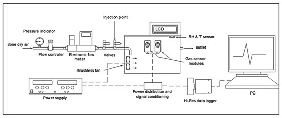
Figure 2.
Gas concentration measurement apparatus.
Regulated dry air was allowed to flow inside the chamber at a rate of 1800 mL/min adjusted with the aid of an electronic flow meter (flow gas mass flow controller Model 32907-75, Cole-Parmer, St. Neots, UK). The purpose of the clean air stream was to remove any moisture from inside the test chamber and isolate it from any contaminants that may interfere with the measurements. In addition, the continuous flow of the air stream kept the sensors in a stable state, providing a virtually constant operating environment for the duration of the experiment. Outflowing gases exited the chamber at the same flow rate through a hole on the opposite side to the inlet.
The measurement process was implemented by first preparing saturated ethanol gas samples from known liquid concentrations, then injecting 3 mL of the saturated gas, taken from calibration samples, into the test chamber by a syringe through the gas mixing valve. Injected vapors were mixed with the dry air stream and fed into the chamber. They became evenly distributed inside the chamber with the aid of the brushless fan. After injection, signals were detected due to the fast change in the conductivity of the sensors. Their conductivity returned back to the initial state when the air inside the chamber became free again from all traces of the injected gas. Calibration curves were made based on the signal peak value of the injected samples. All measurements were carried out at ambient temperature.
After calibration, ethanol vapor samples from the bubble tank were injected in the same way as described above. The unknown concentration of the injected gas can be determined from the calibration curves.
It is appropriate to mention here that we experimentally demonstrated that an air flow rate of 1800 mL/min and a sample injection volume of 3 mL are the suitable operating conditions in our system. They provide reasonable residence times for the samples inside the chamber and enable clear peak heights to be detected at different concentrations whilst ensuring that the gas sensors are not saturated. The rise time for both sensors, i.e., the time taken for the signal to reach maximum height from its base line, was similar for all concentrations studied. Rise times of 19 s–20 s were observed for sensor 1, and of 15 s–19 s for sensor 2. Base line variations (or drift) was in the range 98.173 to 100.518 mV for sensor 1 and 100.716–103.819 mV for sensor 2.
2.3. Measurements of the Liquid Phase Concentration in Ternary Mixtures
The method adapted for measuring the vapor phase in the binary mixtures can be extended for measuring liquid concentrations for the ternary mixture indirectly by vaporizing a known quantity of liquid inside the measuring unit. To achieve this, an electronic nose was developed for this purpose by adding extra sensors to the measuring unit. An electronic nose is a device composed of an array of gas sensors that shows different response patterns when exposed to different gas constituents or concentrations [13,21]. In order to obtain accurate results, the number of sensors in the gas sensor array should be greater than the number of target components in the system [22,23].
Our electronic nose comprised two MikroElektronika MQ-3 (MikroElektronika, Belgrade, Serbia) gas sensor modules and two Figaro TGS2620 (Figaro USA, Inc., Arlington Heights, IL, USA) and one Figaro TGS2610 gas sensors connected to different load resistors in order to change their sensitivity. We also introduced the Honeywell HIH-3610 (Honeywell International Inc., Morris Plains, NJ, USA) humidity sensor to measure water concentration in the samples. An interesting feature about the humidity sensor is that it is a completely independent sensor and does not respond to any compounds in the mixture except water. This makes a total of six sensors—five gas sensors and one humidity sensor—installed in the unit described in Figure 2. The measurements were conducted at ambient temperature.
The suggested model to correlate the concentration of acetic acid and acetol in the mixture was proposed to follow a complete second order degree polynomial regression of two variables as shown in Equation (3). To calculate the polynomial coefficients, the following minimization equation was solved [24,25,26]:
where CA and CB are the acetic acid and acetol concentrations measured in volume percentage (vol%) in the liquid mixture, respectively, M is the total number of gas sensors installed (i.e., 5), N is the number of calibration samples, Sji denotes the sensor responses, and Aj, Bj, Cj, Dj, Ej, Fj are polynomial coefficients.
Once the above equation has been solved and the values of the polynomial coefficients are calculated, the following minimization equation is solved to find the responses of the unknown samples:
in which the unknown values are CA and CB. Water content was calculated as 100CACB and compared with the humidity sensor results as a check for consistency. MATLAB was used to solve the minimization for both equations using the Nelder-Mead amoeba algorithm.
3. Results and Discussion
3.1. Vapor Phase Concentration in Binary Mixtures
Figure 3 demonstrates the dynamic response of the gas sensors for 10 training or calibration samples (vapors from 10 vol% up to 100 vol% of liquid ethanol-water mixtures). As can be seen, the two responses are close to each other, but this is not a necessary condition, even for the same type of sensors, since identical sensor properties cannot be 100% guaranteed during the manufacturing process. Figure 4 shows the calibration curves for each sensor.
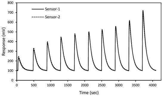
Figure 3.
Dynamic response of gas sensors.
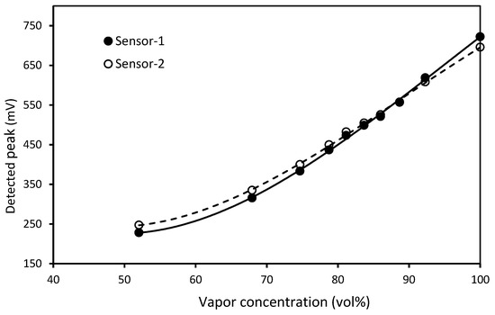
Figure 4.
Gas sensors calibration curves.
The interesting feature that can be extracted from Figure 4 is that the range from 70% and above shows a linear relationship between the gas concentration and the sensor’s response. The R-squared values were calculated to be 0.9965 and 0.9977 respectively for sensors 1 and 2.
Table 1 shows typical numerical results for 14 different samples that were injected randomly into the measuring unit after the calibration process. Ethanol x-y equilibrium data are obtained from the literature [27]. As can be seen, the results show a good degree of accuracy. The maximum error reported is around 1%, and the average error is 0.433%, confirming the reliability of this method for the measurements.

Table 1.
Test sample measurements.
The calculated value of R-squared is 0.9817, which confirms the strong relationship between the measured values and the actual ones. However, values of R-squared higher than 0.99 for an ethanol-water system have been reported [2].
It should be noted that there is an unavoidable drift of the order of a few millivolts in the base line of each sensor. Consequently, all measurements were adjusted in line with the base line average value following the mapping [28]
where is the final value of the signal after correction, represents the highest value of the signal obtained from the injected sample, or simply signal peak value, is the sensor base line of the signal under analysis, and is the average base line of the sensor along the experiment.
3.2. Liquid Phase Concentration in Ternary Mixtures
In the next set of experiments, 20 different interaction samples were prepared. Acetic acid concentrations up to 20 vol% were considered, while acetol concentrations of up to 81 vol% were used. All the responses were based on the evaporation of 1 µL of the liquid mixture inside the chamber using a GC micro syringe (Model: Hamilton 7105KH, Hamilton Company, Reno, NV, USA). Figure 5 and Figure 6 show the actual concentrations and the measured concentrations obtained from Equation (4) for acetic acid and acetol, respectively. The R-squared values were found to be 0.9865 for acetic acid and 0.9987 for acetol.
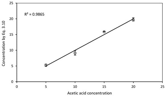
Figure 5.
Graph of the real concentrations of acetic acid versus the estimated ones by Equation (4).
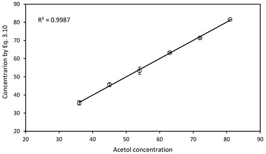
Figure 6.
Graph of the real concentrations of acetol versus the estimated ones by Equation (4).
Table 2 compares water concentration measurements made using a humidity sensor with those calculated from the constraint equation. The R-squared values were found to be 0.9728 for the measurements made using the humidity sensor and 0.98 for data calculated from the constraint equation.
Table 2.
Calibration concentrations of water.
4. Conclusions
Microbubble distillation is inherently a transient process with potentially rapid kinetics creating a difficult challenge for chemosensor systems. A regression-based algorithm was used to test the accuracy of an electronic nose developed to make measurements in the vapor phase for binary systems and in the liquid phase for ternary systems in a microbubble distillation unit. The results demonstrate that our system has the ability to estimate component concentration in both mixtures. The experimental results were in close agreement with the actual composition values, thus confirming the appropriateness and accuracy of the novel sensor design. Future work will be devoted to identifying and qualifying more complex mixtures.
Author Contributions
Conceptualization, N.N.A. and B.H.A.-S.; Formal analysis, N.N.A. and B.H.A.-S.; Methodology, N.N.A. and B.H.A.-S.; Project administration, W.B.Z.; Software, B.H.A.-S.; Supervision, J.M.R. and W.B.Z.; Validation, N.N.A. and B.H.A.-S.; Visualization, J.M.R.; Writing—original draft, N.N.A. and B.H.A.-S.; Writing—review & editing, J.M.R.
Funding
This research was funded by an EPSRC 4CU Programme Grant 4cu.org.uk (EP/K001329/1). Support was also provided from Innovate UK/EPSRC under the IB Catalyst industrial research scheme, EP/N011511/1.
Acknowledgments
N.N.A. thanks the Higher Committee of Education and Development in Iraq for a doctoral scholarship. W.B.Z., N.N.A., and B.H.A. acknowledge support from the ERA-net IB project z-fuels through Perlemax.
Conflicts of Interest
The authors declare no conflict of interest.
References
- Liu, X.; Cheng, S.; Liu, H.; Hu, S.; Zhang, D.; Ning, H. A survey on gas sensing technology. Sensors 2012, 12, 9635–9665. [Google Scholar] [CrossRef] [PubMed]
- Khalaf, W. Sensor Array System for Gases Identification and Quantification. In Recent Advances in Technologies; Strangio, M.A., Ed.; InTech: Rijeka, Croatia, 2009; Available online: http://cdn.intechopen.com/pdfs/9272/InTech-Sensor_array_system_for_gases_identification_and_quantification.pdf (accessed on 25 May 2018).
- Pace, C.; Fragomeni, L.; Khalaf, W. Developments and Applications of Electronic Nose Systems for Gas Mixtures Classification and Concentration Estimation. In Applications in Electronics Pervading Industry, Environmental and Society; De Gloria, A., Ed.; Springer International Publishing: Basel, Switzerland, 2016; pp. 1–7. ISBN 978-3-319-20226-6. [Google Scholar]
- Miecznikowski, J.C.; Sellers, K.F. Statistical Analysis of Chemical Sensor Data. In Advances in Chemical Sensors; Wang, W., Ed.; InTechOpen: London, UK, 2012; ISBN 978-953-307-792-5. [Google Scholar]
- Scott, S.M.; James, D.; Ali, Z. Data analysis for electronic nose systems. Microchim. Acta 2006, 156, 183–207. [Google Scholar] [CrossRef]
- Wilson, A.; Baietto, M. Applications and advances in electronic-nose technologies. Sensors 2009, 9, 5099–5148. [Google Scholar] [CrossRef] [PubMed]
- Pace, C.; Khalaf, W.; Latino, M.; Donato, N.; Neri, G. E-nose development for safety monitoring applications in refinery environment. Procedia Eng. 2012, 47, 1267–1270. [Google Scholar] [CrossRef]
- Kurup, P.U. An electronic nose for detecting hazardous chemicals and explosives. In Proceedings of the 2008 IEEE Conference on Technologies for Homeland Security, Waltham, MA, USA, 12–13 May 2008; Volume 978, pp. 144–149. [Google Scholar] [CrossRef]
- Rudnitskaya, A.; Legin, A. Sensor systems, electronic tongues and electronic noses, for the monitoring of biotechnological processes. J. Ind. Microbiol. Biotechnol. 2008, 35, 443–451. [Google Scholar] [CrossRef] [PubMed]
- Ryabtsev, S.V.; Shaposhnick, A.V.; Lukin, A.N.; Domashevskaya, E.P. Application of semiconductor gas sensors for medical diagnostics. Sens. Actuators B Chem. 1999, 59, 26–29. [Google Scholar] [CrossRef]
- Jiang, H.; Zhang, H.; Chen, Q.; Mei, C.; Liu, G. Recent advances in electronic nose techniques for monitoring of fermentation process. World J. Microbiol. Biotechnol. 2015, 31, 1845–1852. [Google Scholar] [CrossRef] [PubMed]
- Gardner, J.W.; Bartlett, P.N. Performance definition and standardisation of electronic noses. Sens. Actuators B Chem. 1996, 33, 60–67. [Google Scholar] [CrossRef]
- Gardner, J.W.; Bartlett, P.N. Electronic Noses: Principles and Applications; Oxford University Press: New York, NY, USA, 1999; ISBN 9780198559559. [Google Scholar]
- Rock, F.; Barson, N.; Weimar, U. Metal oxide gas sensor arrays: Geometrical design and selectivity. AIP Conf. Proc. 2009, 1137. [Google Scholar] [CrossRef]
- Vargas-Bernal, R. Techniques to optimize the selectivity of a gas sensor. In Proceedings of the Robotics and Automotive Mechanics Conference (CERMA 2007), Morelos, Mexico, 25–28 September 2007. [Google Scholar] [CrossRef]
- Wang, C.; Yin, L.; Zhang, L.; Gao, R. Metal oxide gas sensors: Sensitivity and influencing factors. Sensors 2010, 10, 2088–2106. [Google Scholar] [CrossRef] [PubMed]
- Gardner, J.W. Detection of vapours and odours from a multisensory array using pattern recognition: Part 1. Principal component and cluster analysis. Sens. Actuators B Chem. 1991, 4, 109–115. [Google Scholar] [CrossRef]
- Gardner, J.W.; Hines, E.L.; Tang, H.C. Detection of vapours and odours from a multisensory array using pattern-recognition techniques. Part 2: Artificial neural networks. Sens. Actuators B Chem. 1992, 9, 9–15. [Google Scholar] [CrossRef]
- Abdulrazzaq, N.N.; Al-Sabbagh, B.H.; Rees, J.M.; Zimmerman, W.B. Purification of bioethanol using microbubbles generated by fluidic oscillation: A dynamical evaporation model. Ind. Eng. Chem. Res. 2016, 55, 12909–12918. [Google Scholar] [CrossRef]
- Abdulrazzaq, N.N. Application of Microbubbles Generated by Fluidic Oscillation in the Upgrading of Bio Fuels. Ph.D. Thesis, University of Sheffield, Sheffield, UK, 2016. [Google Scholar]
- Gardner, J.W.; Bartlett, P.N. A brief history of electronic noses. Sens. Actuators B Chem. 1994, 18, 210–211. [Google Scholar] [CrossRef]
- Yang, Y.; Yi, J.; Jin, R.; Mason, A.J. Power-error analysis of sensor array regression algorithms for gas mixture quantification in low-power microsystems. In Proceedings of the 2003 IEEE SENSORS, Baltimore, MD, USA, 3–6 November 2013. [Google Scholar] [CrossRef]
- Khalaf, W.; Pace, C.; Gaudioso, M. Gas detection via machine learning. World Acad. Sci. Eng. Technol. 2008, 37, 139–143. [Google Scholar]
- Khalaf, W.; Pace, C.; Gaudioso, M. Least square regression method for estimating gas concentration in an electronic nose system. Sensors 2009, 9, 1678–1691. [Google Scholar] [CrossRef] [PubMed]
- Zhou, H.; Homer, M.L.; Shevader, A.V.; Ryan, M.A. Nonlinear least-squares based method for identifying and quantifying single and mixed contaminants in air with an electronic nose. Sensors 2006, 6, 1–18. [Google Scholar] [CrossRef]
- Gaudioso, M.; Khalaf, W.; Pace, C. On the use of the SVM approach in analyzing an electronic nose. In Proceedings of the 7th International Conference on Hybrid Intelligent Systems, Kaiserslautern, Germany, 17–19 September 2007; pp. 42–46, ISBN 0-7695-2946-1. [Google Scholar]
- Flick, E. Industrial Solvents Handbook, 5th ed.; William Andrew Noyes Publications: New York, NY, USA, 1998; ISBN 9780815518099. [Google Scholar]
- Di Carlo, S.; Falasconi, M. Drift correction methods for gas chemical sensors in artificial olfaction systems. In Advances in Chemical Sensors; Wang, W., Ed.; IntechOpen: London, UK, 2012; ISBN 978-953-307-792-5. [Google Scholar]
© 2018 by the authors. Licensee MDPI, Basel, Switzerland. This article is an open access article distributed under the terms and conditions of the Creative Commons Attribution (CC BY) license (http://creativecommons.org/licenses/by/4.0/).