Abstract
In this work, a fractional-order synthetic drugs transmission model with psychological addicts has been proposed along with psychological treatment. The effects of synthetic drugs are deadly and sometimes even violent. We have studied the local and global stability of the model with different criterion. The existence and uniqueness criterion along with positivity and boundedness of the solutions have also been established. The local and global stabilities are decided by the basic reproduction number . We have also analyzed the sensitivity of parameters. An optimal control problem has been formulated by controlling psychological addiction and analyzed by the help of Pontryagin maximum principle. These results are verified by numerical simulations.
1. Introduction
Synthetic drugs, also referred to as designer or club drugs, are chemically created in a lab to mimic another group of drugs such as marijuana, cocaine, or morphine. There are more than 200 to 300 identified synthetic drug compounds and many of them are cocaine, methamphetamine, and marijuana compounds [1,2]. The effects of synthetic drugs are anxiety, aggressive behavior, paranoia, seizures, loss of consciousness, nausea, vomiting, and even coma or death [3]. Synthetic drugs are powerful, and when mixed with unknown chemical compounds are extremely dangerous and can cause overdose very quickly. If an overdose has occurred, immediate medical care is required. More lately, new designer drugs have emerged with vigorous addictive potentials such as synthetic cathinones (“Bath Salts”), also labeled as Bliss, Vanilla Sky, and Ivory Wave. These synthetic drugs stimulate the central nervous system by inhibiting the retake of norepinephrine and dopamine, leading to serious adverse effects on the Central Nervous System (CNS) or even death [1]. Moreover, many infectious diseases such as hepatitis and AIDS can easily infect drug users due to the rampant use of shared needles [4,5]. Drugs like amphetamine are mostly used in specific regions like Goa and Ahmedabad in India. A recent study shows that drug use in India continues to grow rapidly, and more disturbingly, heroin has replaced the natural opioids (opium and poppy husk). An epidemiological study from Punjab has been revealed that the use of other synthetic drugs and cocaine has also increased significantly [6]. Most synthetic drugs are manufactured in an illegal laboratory, and there are no safety measures used in the manufacture of synthetic drugs. When an addicted person attempts to quit, he/she may experience very uncomfortable withdrawal symptoms which can lower their resolve to maintain abstinence and otherwise complicate early recovery. Professional detoxification programs are needed for synthetic drug addicts to withdraw safely from synthetic drugs. Behavioral therapies and counseling are effective tools for changing negative behavior and thought patterns that may help for improving the mental help they need.
Ma et al. [7] have developed different forms of heroin epidemic models to study the transmission of heroin epidemics. Sharomi and Gumel [8] have formulated different smoking models for giving up smoking. Similarly, mathematical modeling can be also used to describe the spread of synthetic drugs. Nyabadza et al. [9] have studied the methamphetamine transmission model in South Africa. Liu et al. [10] have formulated a synthetic drug transmission model with treatment and studied global stability and backward bifurcation of the model. Saha and Samanta [11] have also studied the stability of a synthetic drug transmission model with optimal control. There are many works that have been performed on fractional-order epidemiological systems because a fractional-order system has memory effect [12]. Fractional calculus is often utilized for the generalization of their order, where fractional order is replaced with integer order [13]. During a systematic study, it has been noted that the integer order model may be a special case of fractional order model wherever the solution of fractional order system must converge to the solution of integer order system as the order approaches one [14]. There are so many fields where fractional order systems are more suitable than integer order systems. Phenomena that are connected with memory and affected by hereditary cannot be expressed by integer order system [15]. It is observed that the data collected from real-life phenomena fit better with the fractional-order system. Diethelm [16] has compared the numerical solutions of fractional-order system and integer order system, and concluded that the fractional order system gives more relevant interpretation than integer order system. There are many systems [17,18,19,20,21,22] that have been studied recently in fractional order framework. In epidemiology, the Ebola virus model has been studied in Caputo differential equation system in 2015 [23]. Agarwal [24] first studied optimal control problem in fractional order system in 2004. In 2018, Kheiri and Jafari [25] have also worked on fractional order optimal control for HIV/AIDS.
Motivation and Brief Overview
There are some relevant advantages of Caputo fractional differentiations and differential equations.
- Fractional derivatives provide an excellent instrument for the description of memory and hereditary properties of various systems and processes. Fractional-order differential equations accumulate the entire information of the function in weighted form.
- In fractional-order modeling, we have an additional parameter (order of the derivative) which is useful for numerical simulations. In that regard, there are some systems which are stable (unstable) for some parameter values near their equilibrium points can be destabilized (stabilized) by controlling the order of the derivative.
- The Caputo derivative is very useful when dealing with real-world problem because it allows traditional initial and boundary conditions to be included in the formulation of the problem, and in addition the derivative of a constant is zero which does not happen in the Riemann–Liouville fractional derivative.
Motivated by the aforementioned works and the advantages of Caputo fractional-order differential equations, a model of fractional synthetic drug transmission with psychological drug addicts has been formulated in this work using Caputo fractional-order differential equations (Section 2). In this work, we have analyzed the drug transmission model in the fractional-order framework, and the effect of the psychological treatment of the awareness campaign has also been studied by formulating fractional-order optimal control problem.
This work is presented in two different parts. In the first part (Section 3), we first carried out a basic analysis, such as existence, oneness, non-negativity, and the limit of solutions of the proposed system of equations. Dynamical behaviors of the different equilibrium points are established in the same section. Though our main aim is to study the system in fractional-order framework, a fractional-order control problem has also framed in Section 4 to study the control effect of treatment on psychological addict class which may enhance our research.
In the beginning of our work, we recall some basic definitions and theories of fractional-order differential equations (Section 3) followed by calculating equilibrium points (Section 3.1). Next, we also discuss whether the solution of the proposed system is unique (Section 3.2). We have also discussed the boundedness and feasible condition of the solutions of the system (Section 3.3). Transfer dynamics has also been discussed with the help of the reproduction number in the next section (Section 3.5). We also study sensitivity analysis (Section 3.4) of the model with local and global stability of equilibrium points (both disease-free and endemic) systematically (Section 3.6). Then, we present our system as an optimal control problem with psychological treatment as control variable and derived optimal conditions (Section 4). Finally, numerical simulations are performed (Section 5), followed by some conclusions of the whole work (Section 6).
2. Model Formulation
We have formulated a fractional-order synthetic drugs transmission model with psychological addicts by taking susceptible (S), psychological addicts (), physiological addicts (), and treatment class as four compartments.
where is the order of derivative and is notation due to Caputo fractional derivative, and is the initial time. Here, , , , and represent the respective size of susceptible population, psychologically addicted population, physiological addicted population, and the class of addicts in treatment, respectively. From a survey on synthetic drugs, it is evident that a large number of the young population are in the susceptible class, which is roughly equivalent to the recruitment rate A of susceptible class and which is assumed to be constant [26]. After contact with an addict, the susceptible addict will first pass into the class of psychological addict, while after taking many drugs, the psychological addict will become the physiological addict. Broadly speaking, a susceptible addict is more likely to initiate drug abuse when he/she has contact with a physiological addict compared to a psychological addict. We denote the corresponding contact rates are and . Once psychological and physiological addicts accept treatment and rehabilitation, they will enter into treatment compartment. The treatment rates are denoted by and , respectively. In addition, some drug users in treatment may escape and reenter physiologically addicted compartment with rate . The parameters and are the escalation rate from psychological addicts to physiological addicts and natural death rate, respectively. All parameters are assumed to be positive constants (briefly described in Table 1). Schematic diagram of system (3) is mentioned in Figure 1.

Table 1.
Parameters of system (3).
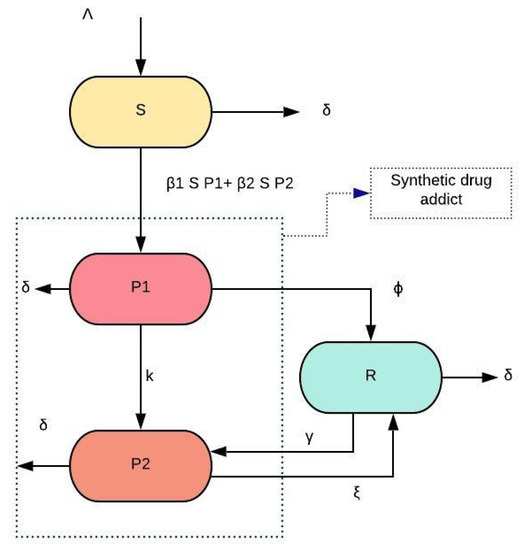
Figure 1.
Schematic diagram of system (3).
It is observed that the time dimension of system (1) is correct because both sides of the equations of system (1) have dimension [27]. Next, let us consider and omit the superscript to all parameters and redefine system (1) as
We have considered to be the total human population and so . In the first phase, a susceptible individual becomes a psychological addict after they come in contact with a drug addict. However, after becomes accustomed to the persistent presence and influence of the drug, the individual is likely to become a physiological addict. A psychological or physiological addict will enter into the treatment compartment at the time of taking treatment and rehabilitation. It is shown in Section 3.3 that the number of total human population is bounded above and let Therefore, we can assume that the total population is constant (N) for large time scale (). Let us scale the state variables with respect to the total population N:
Therefore, system (2) becomes
3. Preliminaries
Definition 1
([28]).The Caputo fractional derivative with order for a function ) is denoted and defined as
where is the Gamma function, and n is a natural number. In particular, for :
Lemma 1.
(Generalized Mean Value Theorem) [29] Let and if is continuous in , then
where , .
Remark 1.
If , then is a non-decreasing (non-increasing) function for .
Definition 2
([13]).One-parametric and two-parametric Mittag–Leffler functions are described as follows:
Theorem 1
([30]).Let . Assume that is continuously differentiable functions up to order on and derivative of exists with exponential order. If is piecewise continuous on , then
where denotes the Laplace transform of .
Theorem 2
([31]).Let be the complex plane. For any and , then
for , where represents the real part of the complex number s, and is the Mittag–Leffler function.
Theorem 3
([28]).Consider the following fractional-order system:
with , and The equilibrium points of this system are evaluated by solving the following system of equations: . These equilibrium points are locally asymptotically stable iff each eigenvalue of the Jacobian matrix calculated at the equilibrium points satisfy .
3.1. Equilibria of System (3)
The equilibria of system (3) can be obtained by solving the system:
System (3) has two types of equilibrium points:
- Drug-free equilibrium
- Drug-addiction equilibrium , where
For drug-addiction equilibrium to exist in feasible region , it is necessary and sufficient that
3.2. Existence and Uniqueness
Lemma 2
([32]).Consider the system:
with initial condition , where , , if local Lipschitz condition is satisfied by with respect to x, then there exists a solution of (6) on which is unique.
To study the existence and uniqueness of system (3), let us consider the region ,where and . Denote and . Consider a mapping , where
For any :
and
Therefore, satisfies Lipschitz’s condition with respect to X. Therefore, Lemma 2 confirms that there exists a unique solution of system (3) with initial condition . The following theorem is the consequence of this result.
Theorem 4.
There exists a unique solution of system (3) for all with initial condition .
3.3. Non-Negativity and Boundedness
In this section, we have established the criterion for feasibility of the solution of system (3). Suppose stands for the set of all non-negative real numbers and represents the first quadrant.
Theorem 5.
(Non-negativity):The solutions of system (3) remain in if .
Proof.
From (7), we have
From Lemma 1, we can say is increasing in a neighborhood of time t where and cannot cross the axis . Therefore, for all . Now, we claim that the solution starts from and remains non-negative. If not, then there exists such that crosses axis at for the first time and the following conditions hold:
From (8), we have . Now, we have two cases
Case 1: If then by the Remark 1 of Lemma 1, we can say that is non-decreasing in a neighborhood of and which concludes . Therefore, we have arrived at a contradiction.
Case 2: If , then there exists a such that with
From (9), we have
Now we have two sub-cases.
Sub-case 1: If , then and it contradicts our assumption.
Sub-case 2: If , then as and must be negative. In this case, we can find a such that with
From (10), we have
which contradicts our assumption that . Therefore, we have .
Again from (9), we have . If then is non-decreasing (remark of Lemma 1) and . If possible, let crosses axis for the first time at . Then, we have
From (10), we have
and this opposes our assumption . Hence . Again from (10), it is evident that and assures that and also , .
Thus, all solutions of system (3) (and thus system (2)) starting in are confined in the region . □
Theorem 6.
(Boundedness):Solutions of system (2) are uniformly bounded.
Proof.
From the first equation of (2), it is noted that
Taking Laplace transforms on both sides, we have
Taking inverse Laplace transforms (using Theorem 2),
where and, as it is from the properties of Mittag–Leffler function [33],
In this case
Let represent the total population, then
Therefore,
Applying Laplace transformation, we have (using Theorem 1):
Taking inverse Laplace transforms (using Theorem 2),
From (12) and (13), we get
where
Thus, are bounded and thus (using Theorem 5) the solutions are bounded uniformly in for □
3.4. Reproduction Number and Sensitivity Analysis
The basic reproduction number is defined as the number of new addicted individuals produced by a single addicted individual during infectious period when contacted into susceptible compartment ( = 2 means a person who has the synthetic drug addiction will transmit it to an average of 2 other people). Reproduction number of system (3) for can be calculated as the maximum eigenvalue of the next generation matrix computed at the drug-free equilibrium [34]. Here,
Thus, we get
The first part is due to the psychologically addicted people and the second part is due to the physiological addicted people.
The drug–addiction equilibrium of system (3) can be rewritten as
Therefore, if , the drug–addict equilibrium exists.
The basic reproduction number of system (3) relies upon seven parameters: per capita contact rates , rate of recruitment (of S), escalation rate from psychological to physiological addicts (k), per capita treatment rates for psychological and physiological addicts respectively (, ), and natural death rate (). Among these parameters, we cannot control the parameters , k, and . Therefore, the basic reproduction number mainly depends on and the value of according to Table 2. To examine the sensitivity of to any parameter (say, ), normalized forward sensitivity index with respect to each parameter has been computed as [11,34]
Table 2.
Sensitivity indices of different parameters of system (3) corresponding to Table 3.
The sensitivity index may depend on some system parameters but also can be constant or independent of some parameters. These values are very important to estimate the sensitivity of parameters, which should be done cautiously, as a small perturbation in a parameter causes relevant quantitative changes. Merely, the estimation of a parameter with a lower sensitivity index does not demand caution, because a small perturbation in that parameter causes small changes. In this context, we have examined the sensitivity of to the parameters , , and , normalized forward sensitivity index with respect to Table 3.
Table 3.
Parameter values used in system (3) when and .
If , where b is a nonzero real number, then
Here, are the sensitivity indexes correspond to the respective parameters . Therefore, it is clear that the basic reproduction number () is most sensitive to changes in ( = 1), where and b is a nonzero real number, probability of transmission from susceptible to drug addicts (both psychological and physiological).
If increases, also increases, whereas decreases when increases, or vice versa. However, the increase in , i.e., the treatment rate for psychological addicts, cannot help as much as the treatment rate for physiological addicts . In this way, it is smarter to concentrate either (the contact rates ) and , treatment rate for mental addicts. It is also noticeable that is more sensitive to rather than according Table 2.
3.5. Local Stability
To analyze the local stability of disease free and endemic equilibrium points, we need the following.
Definition 3
([37]).The discriminant of a polynomial is defined by
Where is the Sylvester matrix of and of order and .
For , we have and .
Therefore,
Lemma 3.
(Routh–Hurwitz conditions for fractional calculus) [38]: If is the discriminant of the characteristic equation of Jacobian matrix of system evaluated at equilibrium point, then for the system is asymptotically stable if any of the following conditions hold:
- 1.
- and
- 2.
- and
- 3.
- and .
To study the local stability of the system (3), we need to compute Jacobian matrices at the equilibrium points and . At the drug-free equilibrium point :
The eigenvalues of the system are , and the other three eigenvalues can be found from the equation , where
Suppose , then by the Routh–Harwitz conditions for the fractional differential equation, the endemic equilibrium point is locally asymptotically stable if any of the following conditions hold:
- and
- and
- and
Jacobian matrix at is given by
Characteristic equation of this matrix is , where
Therefore, , can be found from this equation. Suppose , then by the Routh–Hurwitz conditions for fractional differential equations, the endemic equilibrium point is locally asymptotically stable if any of the following conditions hold:
- and
- and
- and
The following theorems are the consequence of these discussions.
Theorem 7.
The drug-free equilibrium of system (2) is locally asymptotically stable if any of the following conditions holds with (17):
- 1.
- and
- 2.
- and
- 3.
- and .
Here .
Theorem 8.
The endemic equilibrium of system (2) is locally asymptotically stable if any of the following conditions holds with (18) and (19):
- 1.
- and
- 2.
- and
- 3.
- and .
Here, .
3.6. Global Asymptotic Stability
We need following useful lemmas about Lyapunov direct method related with global stability of the equilibrium points in fractional order models.
Lemma 4
([32]).Suppose be a continuous and differentiable function. Then, for any moment of time , .
Lemma 5.
(Uniform Asymptotic Stability Theorem) [39]:
Consider the non-autonomous system
Let be an equilibrium point of the system () and be a continuously differentiable function such that
where Θi, i = 1, 2, 3, are continuous positive definite functions on Ω. Then, the equilibrium point of system (20) is globally asymptotically stable.
Theorem 9.
If , then the disease-free equilibrium of system (3) is globally asymptotically stable when
Proof.
We have considered a positive definite function:
Clearly, and only when .
Taking the order Caputo derivative of L along the solution of system (3), we have (for large time t)
where
Therefore, if . Therefore, using Lemma 5:
Thus, in the limit is given by the solutions of . As the theorem follows. □
Theorem 10.
If , then the endemic equilibrium of system (3) is globally asymptotically stable.
Proof.
Consider a positive definite function:
It is observed that and only at . Taking the order Caputo derivative of V and using Lemma 4, we have
From the steady-state of equilibrium point (4), we have
Let
From (22) and (23), we have
Using the inequality , we have . From relation (24) it is clear that and thus is negative definite with respect to . Thus is globally asymptotically stable by Lemma 5. □
4. Fractional Optimal Control Problem
The applications of Fractional-ordered optimal control problem (FOCP) have grown in recent decades. Agrawal has introduced the general form of FOCPs in the Riemann–Liouville sense and suggests a numerical method to solve FOCP using Lagrange multiplier technique [24]. In traditional integer-order optimal control problems, the calculus of variations is the common method. Pontryagin’s principle is one of the most useful approaches to solve optimal control problem. There are several works where these methods are employed in Fractional ordered optimal control problems [25,40].
Let x be the pseudo-state vector, is the input vector, and U is the set of admissible control of the dynamical system . The system’s pseudo-state is supposed to reach final condition in the unknown final time . The control must be chosen for all to minimize the objective functional J which is defined by the application and can be abstracted as
The constraints on the system dynamics can be adjoined to the Lagrangian F by introducing time-varying Lagrange multiplier vector , whose elements are called the co-states of the system. This motivates the construction of the Hamiltonian H defined for all .
where stands for transpose of . Pontryagin’s minimum principle states that the optimal state trajectory , optimal control , and corresponding Lagrange multiplier vector must minimize the Hamiltonian H so that [41]
- and
where
is the Right Riemann–Liouville derivative of order . The notation “RL” stands for Right Riemann–Liouville derivative. These four conditions are the necessary conditions, but not sufficient for optimal control.
Our point is to limit the number of synthetic drug addicts by considering the impact of “awareness program, mental directing and other preventive measures” as a control strategy. We have thought about system (3) with this control system. Empowering the mindfulness mission and advising program in a successive premise can impact conduct change among mental addicts. Mindfulness crusades keep the populace from ingesting medications as well as make them mindful about the repercussions of engrossing manufactured medications. Considering this, a treatment rate work has been introduced in system (3) to get system (26). Here, c speaks to the therapy rate (through directing) alongside the effect of awareness missions and is the power of treatment. There are various costs included like analysis, drugs, and different costs when advising is given. In this way, can be utilized as a potential instrument to create a constructive outcomes on mental addicts with . Here, 0 portrays no improvement throughout the directing time frame, while 1 is speaking to full improvement. Consequently, the control force completely depends on the exertion of the mental addicts to prevent themselves from consuming synthetic drugs.
In the following, we have focus on determining the optimal treatment via counseling with minimum cost by implementing the control. From the previous discussions, we have deduced that the acceptable set for the control variable is
where represents the final time up to which the control policy can be implemented. It is assumed that the control functions is measurable.
Our main objective is to minimize the given objective function J, which represents cost involved in counseling and awareness programs in time interval , by finding optimal control as follows:
Here,
(where are the cost of treatment of psychological class and cost of implementation of control strategy, respectively )
subject to
The existence of optimal control can be established in the next theorem.
Theorem 11.
Let the control function be measurable on with value of each of lies in [0,1]. Then, there exist adjoint variables and optimal control minimizing the objective function of (26) satisfying
with transversality conditions and
where are the corresponding optimal state solutions of (26) associated with control variable η.
Proof.
We have constructed the Hamiltonian as
with being the associated adjoint variables with , which satisfy the following canonical equations:
Therefore, the problem of finding that minimizes J subject to (26) is converted to minimizing the Hamiltonian with respect to the control. Then, by Pontryagin principle, we have achieved the optimal condition:
which can be solved in terms of the state and adjoint variables to give
For the optimal control , which requires considering the constrains on the control and the sign of , we have
and
The optimal state can be found by substituting into the system (26). □
5. Numerical Simulations
Analytical study is incomplete without numerical verification of the results. In this section, we have presented numerical simulation of system (3) and fractional order control problem (27). We have used FDE12 MatLab function which is designed on predictor–corrector scheme based on Adams–Bashforth–Moulton algorithm introduced by Roberto Garrappa [42]. Diethelm [16,43] used the predictor–corrector scheme based on Adams–Bashforth–Moulton algorithm which is used in FDE12. We have used FDE12 function directly for system (3) just like ODE45, ODE23.
We have also used iterative scheme (Euler’s forward and backward) in MatLab interface to develop fractional order optimal control problem. The process is briefly described below. The optimality system constitutes a two-point boundary value problem including a set of fractional-order differential equations. The state system (26) is an initial value and the adjoint system (29) is a boundary value problem. The state system is solved by forward iteration method and the costate system is solved by backward iteration method by the following algorithm through Matlab.
State system (26) is solved using the iterative scheme below:
where and and is the time step length. Here, is the value of at th iteration. The last term of each of the above system of equations stands for memory. The adjoint system (29) is solved by backward iteration method with terminal conditions using the following iterative scheme:
The optimal control is updated by the scheme below.
We have developed MatLab code using the above algorithm and chosen throughout the numerical simulation. In fitting the test data of memory phenomena from different fields, it has been found that the fractional order can be physically explained as an index of memory. The higher the value of order , the slower the forgetting is and most of the epidemic transmission dynamics depend on memory (previous stages) [15]. The value of order of fractional derivative () needs to be close to 1. Theoretically, we may study the fractional order system for any value lies between 0 to 1, but it is better to choose the value close to 1. There are some cases where we have found interesting results if we reduce the order of derivative, but for very small values of (less than 0.5) the MatLab code become erroneous. Therefore, we have to chose the order wisely and in our context we choose the value 0.95 (it may be any value from 0.9 to 0.99) for numerical simulation. The value of the order can be estimated by least-squares method of curve fitting with real data from field survey or by graphical study [21].
In this section, we have portrayed some time series of system (3) and variation of with respect to . Next, we have discussed about the effect of control intervention. Figure 2 represents the situation when the drug free equilibrium is asymptotically stable corresponds to the Table 3. Next, let us consider the following three cases:
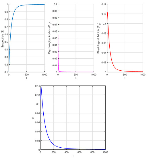
Figure 2.
Time series of system (3) corresponds to Table 2 when and .
Figure 3 depicts the time series and phase portrait of system (3) (case 1) when the drug addict equilibrium is and . Figure 4 and Figure 5 represent the cases 2 and 3 when corresponding equilibrium points are
respectively. Figure 6 represents the variation of time series of state variables when varies and other parameters are fixed as in Table 5. Figure 7, Figure 8, Figure 9 and Figure 10 depict the change in with respect to parameters , respectively. Figure 2 and Figure 3 justify Theorems 7 and 8, respectively. Figure 11 depicts the variation of time series with the control parameter .
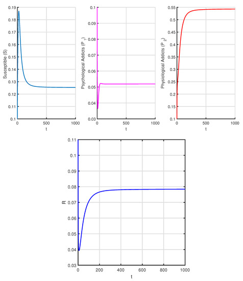
Figure 3.
Time series of system (3) corresponds to Table 3 when and .
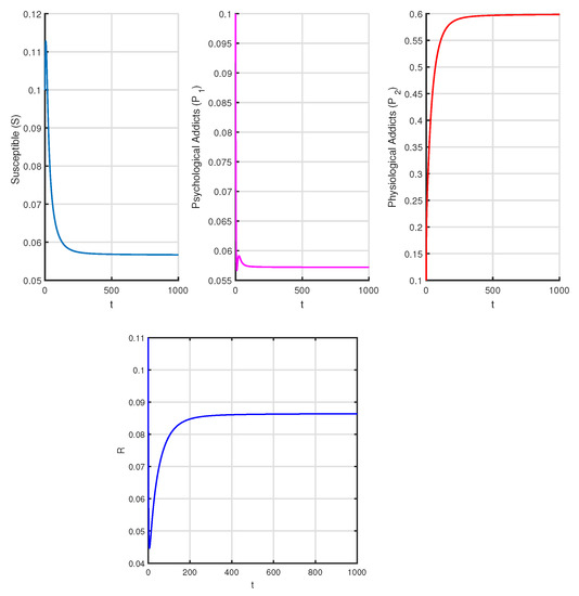
Figure 4.
Time series of system (3) corresponds to Table 4 when and .
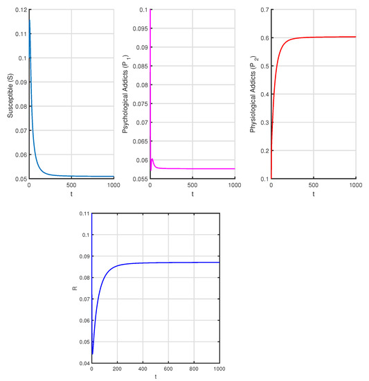
Figure 5.
Time series of system (3) corresponds to Table 5 when and .
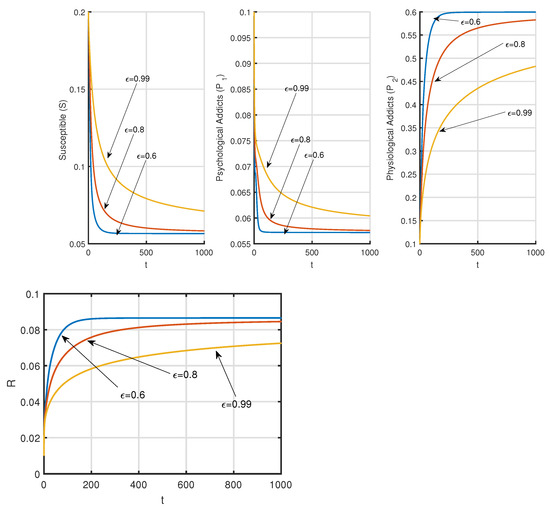
Figure 6.
Variation of time series of system (3) with corresponds to Table 4 when .
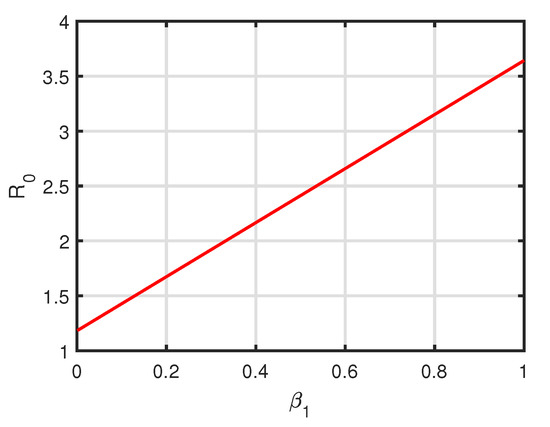
Figure 7.
Variation of of system (3) with respect to while values of other parameters are taken from Table 3.
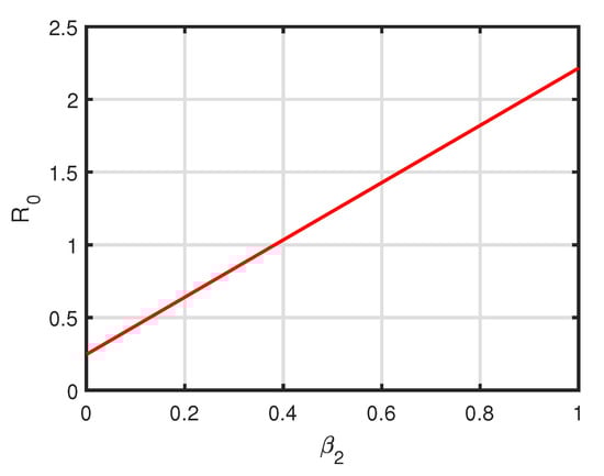
Figure 8.
Variation of of system (3) with respect to while values of other parameters are taken from Table 3.
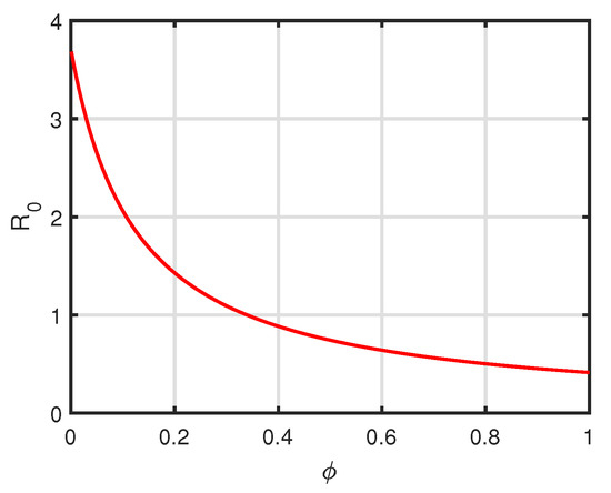
Figure 9.
Variation of of system (3) with respect to while values of other parameters are taken from Table 3.
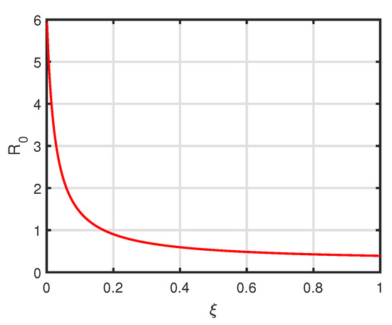
Figure 10.
Variation of of system (3) with respect to while values of other parameters are taken from Table 3.
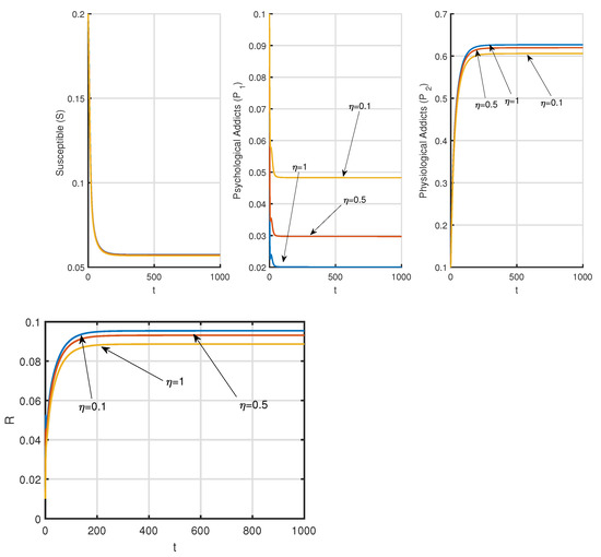
Figure 11.
Variation of time series of system (26) with different control corresponds to Table 4.
Now, let us consider Table 7 for simulating optimal control problem (26). We have used Forward-backward iterative scheme to solve this optimal control problem [44]. For , the drug-free equilibrium point is and . We have considered final time days and day. Note that there are more addicted population in physiological state than in psychological state. Now, we shall discuss about the effect of control intervention. The positive weights have been considered as . Figure 11 shows the variation of time series of state variables when the control parameter changes. Figure 12 represents the time series of state variables of optimal control problem (26). Figure 13 represents time series of optimal control variable () and optimal cost function (). Figure 14 depicts the case when no control is applied. There is a significant number of psychological and physiologically addicted population present in the scenario () which will create economic burden in terms of loss of productivity, morbidity, and mortality and in obtaining protective measures (Figure 14). It has been found from Figure 13 and Figure 14 that if the control strategy is applied, then the number of psychologically addicts and number of addicts in treatment class decrease but the number of physiological addicts increases. The values of in the without control stage after 20 days are 0.5823, 0.003934,0.01343, and 0.023, respectively, but after applying control those values change to 0.5823, 0.003917, 0.01345, and 0.02297. Though the change is smaller in fraction, it is effective in large populated countries like India and China. In Figure 13, it has been observed that the value of optimal control is increasing between 0 to 8 days and then decreases. A certain time is required to persuade a psychologically addicted person that ingesting drugs in a frequent manner is harmful and can even cause physical damages. However, once a person starts understanding these deadly affects, it becomes easy for them to take medicines and to do the other needful to make them free of this addiction. We have performed the cost design analysis for optimal control policy mentioned in Figure 13.
Table 7.
Parametric values used in system (26).
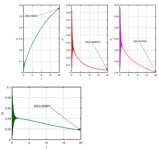
Figure 12.
Time series of state variables of system (26) for Table 6 when , .
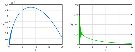
Figure 13.
Time series of optimal control and optimal cost of system (26) for Table 6 when , .
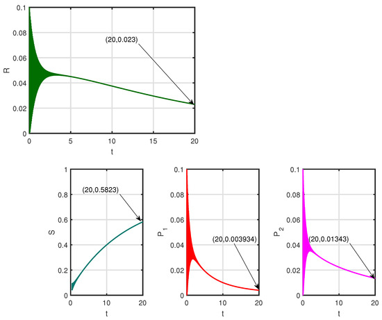
Figure 14.
Time series of state variables of system (26) for Table 6 when and .
6. Conclusions
Fractional calculus plays an important role in dynamical processes. It gives us an extra parameter by which we can simulate our model properly. Here, we have studied on the fractional-order synthetic drugs transmission model with psychological addicts incorporating memory effects. We have observed that the dynamics of system (3) depends on the strength of memory effects, controlled by the order of fractional derivative [13].
In our work, we have framed a model in Caputo-fractional differentiation formalism where people are addicted to drugs both psychologically and physiologically. By next-generation matrix method, we have found the basic reproduction number , and this gives (or, is consistent with) the local and global stability conditions of the drug-free and drug addiction equilibria. It has been observed from numerical examples that if , the system has only drug-free equilibrium and this equilibrium is stable (Figure 2). If , the drug addiction equilibrium persists and locally stable (Figure 3, Figure 4 and Figure 5). By analyzing sensitivity of parameters , we have reached the conclusion that controlling the transmission of the synthetic drugs is better than providing treatment to the addicts. Therefore, we have designed a control strategy to prevent drug transmission. From Figure 6, it has also been found that by lowering the value of fractional order, susceptible and psychological addicted populations decrease but the physiological population and population in treatment class increase.
In the next section of this work, we have discussed an optimal control problem related to the drug abuse epidemic model where we have tried to minimize the drug-addicted population along with the cost of treatment. We have reformulated our model by considering the effect of “counseling and awareness campaigns” as control variable and calculated the total cost. Analytically, we have used Pontryagin’s Principle for fractional calculus to determine the value optimal control parameter [45]. The analytical results and numerical simulations are quite relevant, and by the numerical computations we can deduce certain observations that have been discussed earlier.
Nowadays, an enormous number of the populace, particularly the young population, is presented to the universe of medications because of different reasons. For guiding purposes, we hope to hone in on those populaces. As by taking a gander at them as a helpless populace, it is easier to evaluate how to best acquaint normal guiding with the mental addicts in the general public through the model. Instructive foundations and families should remind adolescents about the significance of well-being training just as the Government needs to assume some responsibility to build mindfulness among the individuals. In goodness of missions and social projects, individuals may understand the human impacts of manufactured medications and decrease interest, which could prompt a lower contact rate. The proposed model shows the effect of guiding mental addicts through mathematical re-enactments. Besides, the result of an ideal reaction because of directing can limit the cost to, and quantity of, dependent people. The approach can limit the general monetary burden. In this circumstance, we ask a legitimate control strategy which will be powerful in the feeling of the study of disease transmission and financial matters.
Author Contributions
All the authors have participate equally in all the aspects of this paper: conceptualization, methodology, investigation, formal analysis, writing—original draft preparation, writing—review and editing. All authors have read and agreed to the published version of the manuscript.
Funding
This research was funded by the Spanish Government for its support through grant RTI2018-094336-B-100 (MCIU/AEI/FEDER, UE) and to the Basque Government for its support through grant IT1207-19.
Institutional Review Board Statement
Not applicable.
Informed Consent Statement
Not applicable.
Data Availability Statement
The data used to support the findings of this study are included in the references within the article.
Acknowledgments
The authors are grateful to the anonymous referees and Nemo Guan, Special Issue Editor, for their careful reading, valuable comments, and helpful suggestions, which have helped them to improve the presentation of this work significantly. The third author (Manuel De la Sen) is grateful to the Spanish Government for its support through grant RTI2018-094336-B-100 (MCIU/AEI/FEDER, UE) and to the Basque Government for its support through grant IT1207-19.
Conflicts of Interest
The authors declare no conflict of interest.
References
- Creagh, S.; Warden, D.; Latif, M.A.; Paydar, A. The New Classes of Synthetic Illicit Drugs Can Significantly Harm the Brain: A Neuro Imaging Perspective with Full Review of MRI Findings. Clin. Radiol Imaging J. 2018, 2, 000116. [Google Scholar] [PubMed]
- “WHAT IS A SYNTHETIC DRUG?” Foundation for a Drug-Free World. Available online: https://www.drugfreeworld.org/drugfacts/synthetic.html (accessed on 21 March 2020).
- The Dangers of Synthetic Drugs. Psycom, University of California, Berkeley Health and Wellness Publications. Available online: https://www.psycom.net/the-dangers-of-synthetic-drugs (accessed on 21 March 2020).
- Garten, R.; Lai, S.; Zhang, J. Rapid transmission of hepatitis C virus among young injecting heroin users in southern China. Int. J. Epidemiol. 2004, 33, 182–188. [Google Scholar] [CrossRef] [PubMed]
- Kapp, C. Crystal Meth Boom Adds to South Africa’s Health Challenges; Lancet: London, UK, 2008; Volume 37, pp. 193–194. [Google Scholar]
- Avasthi, A.; Ghosh, A. Drug misuse in India: Where do we stand & where to go from here? Indian J. Med. Res. 2019, 149, 689–692. [Google Scholar] [CrossRef]
- Ma, M.; Liu, S.; Xiang, H.; Li, J. Dynamics of synthetic drugs transmission model with psychological addicts and general incidence rate. Phys. A Stat. Mech. Its Appl. 2017, 491. [Google Scholar] [CrossRef]
- Sharomi, O.; Gumel, A.B. Curtailing smoking dynamics: A mathematical modeling approach. Appl. Math. Comput. 2008, 195, 475–499. [Google Scholar] [CrossRef]
- Nyabadza, F.; Njagarah, J.B.H.; Smith, R.J. Modelling the dynamics of crystal meth (‘tik’) abuse in the presence of drug-supply chain in South Africa. Bull. Math. Biol. 2013, 75, 24–28. [Google Scholar] [CrossRef]
- Liu, P.; Zhang, L.; Xing, Y. Modelling and stability of a synthetic drugs transmission model with relapse and treatment. J. Appl. Math. Comput. 2019, 60, 465–484. [Google Scholar] [CrossRef]
- Saha, S.; Samanta, G.P. Synthetic drugs transmission: Stability analysis and optimal control. Lett. Biomath. 2019. [Google Scholar] [CrossRef]
- Mainardi, F. On some properties of the Mittag-Leffler function Eα,1(-tα), completely monotone for t>0 with 0<α<1. Discret. Contin. Dyn. Syst. Ser. B 2014, 19, 2267–2278. [Google Scholar] [CrossRef]
- Podlubny, I. Fractional Differential Equations; Academic Press: San Diego, CA, USA, 1999. [Google Scholar]
- Teodoro, G.S.; Machado, J.T.; de Oliveira, E.C. A review of definitions of fractional derivatives and other operators. J. Comput Phys. 2019, 388, 195–208. [Google Scholar] [CrossRef]
- Du, M.; Wang, Z.; Hu, H. Measuring memory with the order of fractional derivative. Sci Rep. 2013, 3, 3431. [Google Scholar] [CrossRef]
- Diethelm, K. Efficient Solution of Multi-Term Fractional Differential Equations Using P(EC)mE Methods. Computing 2003, 71, 305–319. [Google Scholar] [CrossRef]
- Das, M.; Maiti, A.; Samanta, G.P. Stability analysis of a prey-predator fractional order model incorporating prey refuge. Ecol. Genet. Genom. 2018, 7–8, 33–46. [Google Scholar] [CrossRef]
- Das, M.; Samanta, G.P. A prey-predator fractional order model with fear effect and group defense. Int. J. Dyn. Control 2020. [Google Scholar] [CrossRef]
- Das, M.; Samanta, G.P. A delayed fractional order food chain model with fear effect and prey refuge. Math. Comput. Simul. 2020, 178, 218–245. [Google Scholar] [CrossRef]
- Das, M.; Samanta, G.P. Optimal Control of Fractional Order COVID-19 Epidemic Spreading in Japan and India 2020. Biophys. Rev. Lett. 2020, 15, 207–236. [Google Scholar] [CrossRef]
- Das, M.; Samanta, G.P. Stability analysis of a fractional ordered COVID-19 model. Comput. Math. Biophys. 2021, 9, 22–45. [Google Scholar] [CrossRef]
- Das, M.; Samanta, G.P. A Fractional Order COVID-19 Epidemic Transmission Model: Stability Analysis and Optimal Control (5 June 2020). Available online: https://ssrn.com/abstract=3635938 (accessed on 20 February 2021).
- Area, I.; Batarfi, H.; Losada, J.; Nieto, J.J.; Shammakh, W.; Torres, A. On a fractional order Ebola epidemic model. Adv. Diff. Equat. 2015, 278. [Google Scholar] [CrossRef]
- Agarwal, O.P. A general formulation and solution scheme for fractional optimal control problems. Nonlinear Dyn. 2004, 38, 323–337. [Google Scholar] [CrossRef]
- Kheiri, H.; Jafari, M. Optimal control of a fractional order model for the HIV/AIDS epidemic. Int. J. Biomath. 2018, 11, 1850086. [Google Scholar] [CrossRef]
- Kelly, A.; Carvalho, M.; Teljeur, C. Prevalence of Opiate Use in Ireland 2006: A 3-Source Capture Recapture Study; Report Submitted to the National Advisory Committee on Drugs Sub-Committee on Prevalence; Stationery Office: Dublin, Ireland, 2010. [Google Scholar]
- Dokoumetzidis, A.; Magin, R.; Macheras, P. A commentary on fractionalization ofmulti-compartmental models. J. Pharmacokinet Pharmacodyn 2010, 37, 203–207. [Google Scholar] [CrossRef] [PubMed]
- Petras, I. Fractional-Order Nonlinear Systems: Modeling Aanlysis and Simulation; Higher Education Press: Beijing, China, 2011. [Google Scholar]
- Odibat, Z.; Shawagfeh, N. Generalized Taylor’s formula. Appl. Math. Comput. 2007, 186, 286–293. [Google Scholar] [CrossRef]
- Liang, S.; Wu, R.; Chen, L. Laplace transform of fractional order differential equations. Electron. J. Differ. Equ. 2015, 2015, 1–15. [Google Scholar]
- Kexue, L.; Jigen, P. Laplace transform and fractional differential equations. Appl. Math. Lett. 2011, 24, 2019–2023. [Google Scholar] [CrossRef]
- Li, Y.; Chen, Y.; Podlubny, I. Stability of fractional-order nonlinear dynamic systems: Lyapunov direct method and generalized Mittag-Leffler stability. Comput. Math. Appl. 2010, 59, 1810–1821. [Google Scholar] [CrossRef]
- Haubold, H.J.; Mathai, A.M.; Saxena, R.K. Mittag-Leffler functions and their applications. J. Appl. Math. 2011, 2011, 298628. [Google Scholar] [CrossRef]
- Van den Driessche, P.; Watmough, J. Reproduction numbers and sub-threshold endemic equilibria for compartmental models of disease transmission. Math. Biosci. 2002, 180, 29–48. [Google Scholar] [CrossRef]
- Gaff, H.; Schaefer, E. Optimal control applied to vaccination and treatment strategies for various epidemiological models. Math. Biosci. Eng. 2009, 6, 469–492. [Google Scholar] [PubMed]
- Kalula, A.S.; Nyabadza, F. A theoretical model for substance abuse in the presence of treatment. S. Afr. J. Sci. 2011, 108, 96–107. [Google Scholar]
- Gelf, I.M.; Kapranov, M.M.; Zelevinsky, A.V. Discriminants, Resultants, and Multidimensional Determinants; Birkhäuser: Boston, MA, USA, 1994; ISBN 978-0-8176-3660-9. [Google Scholar]
- Ahmed, E.; El-Sayed, A.M.A.; El-Saka, H. On some Routh-Hurwitz conditions for fractional order differential equations and their applications in Lorenz, Rössler, Chua and Chen systems. Phys. Lett. A 2006, 358, 1–4. [Google Scholar] [CrossRef]
- Delavari, H.; Baleanu, D.; Sadati, J. Stability analysis of Caputo fractional-order non linear system revisited. Nonlinear Dyn. 2012, 67, 2433–2439. [Google Scholar] [CrossRef]
- Tabatabaei, S.S.; Yazdanpanah, M.J.; Tavazoei, M.S. Formulation and Numerical Solution for Fractional Order Time Optimal Control Problem Using Pontryagin’s Minimum Principle. IFAC-PapersOnLine 2017, 50, 9224–9229. [Google Scholar] [CrossRef]
- Guo, T.L. The Necessary Conditions of Fractional Optimal Control in the Sense of Caputo. J. Optim. Theory Appl. 2013, 156, 115–126. [Google Scholar] [CrossRef]
- Garrappa, R. On linear stability of predictor-corrector algorithms for fractional differential equations. Internat. J. Comput. Math. 2010, 87, 2281–2290. [Google Scholar] [CrossRef]
- Diethelm, K.; Ford, N.J.; Freed, A.D. A Predictor-Corrector Approach for the Numerical Solution of Fractional Differential Equations. Nonlinear Dyn. 2002, 29, 3. [Google Scholar] [CrossRef]
- Cao, X.; Datta, A.; Al Basir, F. Fractional-order model of the disease Psoriasis: A control based mathematical approach. J. Syst. Sci. Complex 2016, 29, 1565–1584. [Google Scholar] [CrossRef]
- Kamocki, R. Pontryagin maximum principle for fractional ordinary optimal control problems. Math. Methods Appl. Sci. 2014, 37. [Google Scholar] [CrossRef]
Publisher’s Note: MDPI stays neutral with regard to jurisdictional claims in published maps and institutional affiliations. |
© 2021 by the authors. Licensee MDPI, Basel, Switzerland. This article is an open access article distributed under the terms and conditions of the Creative Commons Attribution (CC BY) license (http://creativecommons.org/licenses/by/4.0/).