Qualitative Properties of Randomized Maximum Entropy Estimates of Probability Density Functions

Abstract

The problem of randomized maximum entropy estimation for the probability density function of random model parameters with real data and measurement noises was formulated. This estimation procedure maximizes an information entropy functional on a set of integral equalities depending on the real data set. The technique of the Gâteaux derivatives is developed to solve this problem in analytical form. The probability density function estimates depend on Lagrange multipliers, which are obtained by balancing the model’s output with real data. A global theorem for the implicit dependence of these Lagrange multipliers on the data sample’s length is established using the rotation of homotopic vector fields. A theorem for the asymptotic efficiency of randomized maximum entropy estimate in terms of stationary Lagrange multipliers is formulated and proved. The proposed method is illustrated on the problem of forecasting of the evolution of the thermokarst lake area in Western Siberia.

1. Introduction

Estimating the characteristics of models is a very popular and, at the same time, important problem of science. This problem arises in applications with unknown parameters, which have to be estimated somehow using real data sets. In particular, such problems have turned out to be fundamental in machine learning procedures [1,2,3,4,5]. The core of these procedures is a parametrized model trained by statistically estimating the unknown parameters based on real data. Most of the econometric problems associated with reconstructing functional relations and forecasting also reduce to estimating the model parameters; for example, see [6,7].

The problems described above are solved using traditional mathematical statistics methods, such as the maximum likelihood method and its derivatives, the method of moments, Bayesian methods, and their numerous modifications [8,9].

Among the mathematical tools for parametric estimation mentioned, a special place is occupied by entropy maximization methods for finite-dimensional probability distributions [10,11].

Consider a random variable x taking discrete values $x_1,\cdots ,x_n$ with probabilities $p_1,\cdots ,p_n,$ respectively, and r functions $f_1\left(x\right),\cdots ,f_r\left(x\right)$ of this variable with discrete values. The discrete probability distribution function $\mathbf{p}\left(x\right)=\{p_1\left(x_1\right),\cdots ,p_n\left(x_n\right)\}$ is defined as the solution of the problem

$$H\left(\mathbf{p}\right)=-\sum _{i=1}^n{p}_{i}ln{p}_i,\sum _{i=1}^n{p}_i{f}_k\left(x_i\right)\le q_k,k=1,\cdots ,r,$$

where $q_1,\cdots ,q_r$ are given constants.

If $f_k\left(x_i\right)\equiv x_i^k,$ then the system of equalities specifies constraints on the kth moments of the discrete random variable $x.$ In the case of equality constraints, some modifications of this problem adapted to different applications were studied in [10,11,12,13]. Since this problem is conditionally extremal, it can be solved using the Lagrange method, which leads to a system of equations for Lagrange multipliers. The latter often turn out to be substantially nonlinear functions, and hence, rather sophisticated techniques are needed for their numerical calculation [14,15].

In the case of inequality constraints, this problem belongs to the class of mathematical programming problems [16].

The entropy maximization principle is adopted to estimate the parameters of a priori distributions when constructing Bayesian estimates [17,18] or maximum likelihood estimates.

The parameters of probability distributions (continuous or discrete) can be estimated using various mathematical statistics methods, including the method of entropy maximization. Their efficiency in hydrological problems was compared in [19]. Apparently, the method of entropy maximization yields the best results in such problems due to the structure of hydrological data.

The problem of estimating some model characteristics on real data was further developed in connection with the appearance of new machine learning methods, called randomized machine learning (RML) [20]. They are based on models with random parameters, and it is necessary to estimate the probability density functions of these parameters. The estimation algorithm (RML algorithm) is formulated in terms of functional entropy-linear programming [21].

The original statement of this problem was to estimate probability density functions (PDFs) in RML procedures. However, in recent times, a more general context has been assumed—the method of maximizing entropy functionals for constructing estimates of continuous probability density functions using real data (randomized maximum entropy (RME) estimation).

In this paper, the general RME estimation problem is formulated; its solutions, numerical algorithms, and the asymptotic properties of the solutions are studied. The theoretical results are illustrated by an important application—estimating the evolution of the thermokarst lake area in Western Siberia.

2. Statement of the RME Estimation Problem

Consider a scalar continuous function $\phi (x,\theta )$ with parameters $\theta =\{{\theta }_1,\cdots ,{\theta }_n\}.$ Assume that this function is a characteristic of an object’s model with an input x and an output $\widehat{y}$. Let ${\mathbf{x}}^{\left(r\right)}=\{x\left[1\right],\cdots ,x\left[r\right]\}$ and ${\mathbf{y}}^{\left(r\right)}=\{y\left[1\right],\cdots ,y\left[r\right]\}$ be given measurements at time $t=1,\cdots ,r$. Note that the latter measurements are obtained with random vector errors $\xi =\left\{\xi \right[1],\cdots ,\xi [r\left]\right\},$ which are generally different for different time points.

Thus, after r measurements, the model and observations are described by the equations

$$\begin{array}{ccc}\hfill \widehat{\mathbf{y}}& =& \Gamma ({\mathbf{x}}^{\left(r\right)},\theta ),\hfill \\ \hfill \widehat{\mathbf{v}}& =& \widehat{\mathbf{y}}+\xi ,\hfill \end{array}$$

(1)

where the vector function $\Gamma ({\mathbf{x}}^{\left(r\right)},\theta )$ has the components $\phi \left(x\right[t],\theta )$, where $t=1,\cdots ,r$ are the time points; $\widehat{\mathbf{v}}$ denotes the observed output of the model containing measurement noises of the object’s output.

Let us introduce a series of assumptions necessary for further considerations.

• The random parameters are $\theta \in \Theta \subset R^n,\Theta =[{\theta }^{-},{\theta }^{+}]$, where $[•,•]$ is a vectorial segment in the space $R^n$ [22].
• The PDF $P\left(\theta \right)$ of the parameters is continuously differentiable on its support $\Theta .$
• The random noise is $\xi \in \Xi \subset R^r,$ where

  $$\Xi =\underset{t=1}{\overset{r}{⨂}}{\Xi }_t,{\Xi }_t=[{\xi }_t^{-},{\xi }_t^{+}].$$

  (2)
• The PDF $Q\left(\xi \right)$ of the measurement noises is continuously differentiable on the support $\Xi$ and also has the multiplicative structure

  $$Q\left(\xi \right)=\prod _{t=1}^r{Q}_t\left(\xi \left[t\right]\right).$$

  (3)

The estimation problem is stated as follows: Find the estimates of the PDFs $P^{*}\left(\theta \right)$ and $Q^{*}\left(\xi \right)$ that maximize the generalized information entropy functional

$$\mathcal{H}[P\left(\theta \right),Q\left(\xi \right)]=-{\int }_{Q}P\left(\theta \right)lnP\left(\theta \right)d\theta -\sum _{t=1}^r{\int }_{{\Xi }_t}{Q}_t\left(\xi \left[t\right]\right)ln{Q}_t\left(\xi \left[t\right]\right)\Rightarrow max$$

(4)

subject to

—the normalization conditions of the PDFs given by

$${\int }_{\Theta }P\left(\theta \right)d\theta =1;{\int }_{{\Xi }_t}{Q}_t\left(\xi \left[t\right]\right)d\xi \left[t\right]=1,t=1,\cdots ,r;$$

(5)

and

—the empirical balance conditions

$$\begin{array}{ccc}\hfill \Phi \left[P\right(\theta ),Q(\xi \left)\right]& =& {\mathbf{y}}^{\left(r\right)},\hfill \\ \hfill \Phi \left[P\right(\theta ),Q(\xi \left)\right]& =& \{{\Phi }_1[P\left(\theta \right),Q\left(\xi \right)],\cdots ,{\Phi }_r[P\left(\theta \right),Q\left(\xi \right)]\}\hfill \\ \hfill {\Phi }_t[P\left(\theta \right),Q\left(\xi \right)]& =& {\int }_{\Theta }\phi (x\left[t\right],\theta )P\left(\theta \right)d\theta +{\int }_{{\Xi }_t}{Q}_t\left(\xi \left[t\right]\right)\xi \left[t\right]d\xi \left[t\right],t=1,\cdots ,r,\hfill \end{array}$$

(6)

where ${\mathbf{y}}^{\left(r\right)}=\{y\left[1\right],\cdots ,y\left[r\right]\}$ are the measured data on the object’s output. We will denote the problems (4)–(6) as the RME estimate.

Problems (4)–(6) are of the Lyapunov type [23,24], as they have an integral functional and also integral constraints.

3. Optimality Conditions

The optimality conditions in optimization problems of the Lyapunov type are formulated in terms of Lagrange multipliers. In addition, the Gâteaux derivatives of the problem’s functionals are used [25].

The Lagrange functional is defined by

$$\begin{array}{ccc}\hfill \mathcal{L}\left[P\right(\theta ),Q(\xi ),\mu ,\eta ,\lambda ]& =& \mathcal{H}[P\left(\theta \right),Q\left(\xi \right)]+\mu \left(1-{\int }_{\Theta }P\left(\theta \right)d\theta \right)+\hfill \\ & +& \sum _{t=1}^r{\eta }_t\left(1-{\int }_{{\Xi }_t}{Q}_t\left(\xi \left[t\right]\right)d\xi \left[t\right]\right)+\hfill \\ & +& \sum _{t=1}^r{\lambda }_t\left(y\left[t\right]-{\int }_{\Theta }P\left(\theta \right)\phi (x\left[t\right],\theta )d\theta -{\int }_{{\Xi }_t}{Q}_t\left(\xi \left[t\right]\right)\xi \left[t\right]d\xi \left[t\right]\right).\hfill \end{array}$$

(7)

Let us recall the technique for obtaining optimality conditions in terms of the Gâteaux derivatives [26].

The PDFs $P\left(\theta \right)$ and $Q_t\left(\xi \left[t\right]\right)$, $(t=1,\cdots ,r),$ are continuously differentiable, i.e., belong to the class $C^1.$ Choosing arbitrary functions $h\left(\theta \right)$ and $w_t\left(\xi \left[t\right]\right)$, $(t=1,\cdots ,r),$ from this class, we represent the PDFs as

$$P\left(\theta \right)=P^{*}\left(\theta \right)+\alpha h\left(\theta \right);Q_t\left(\xi \left[t\right]\right)=Q_t^{*}\left(\xi \left[t\right]\right)+{\beta }_t{w}_i\left(\xi \left[t\right]\right),t=1,\cdots ,r,$$

where the PDFs $P^{*}\left(\theta \right)$ and $Q_t^{*}\left(\xi \left[t\right]\right)$ are the solutions of problems (4)–(6), and $\alpha$ and ${\beta }_1,\cdots ,{\beta }_r$ are parameters.

Next, we substitute the above representations of the PDFs into (7). If all functions from $C^1$ are assumed to be fixed, the Lagrange functional depends on the parameters $\alpha$ and ${\beta }_1,\cdots ,{\beta }_r$. Then, the first-order optimality conditions for the functional (7) in terms of the Gâteaux derivative take the form

$$\frac{d\mathcal{L}}{d\alpha }{|}_{(\alpha ,\beta )=0}=0,\frac{\partial \mathcal{L}}{\partial {\beta }_t}{|}_{(\alpha ,\beta )=0}=0,t=1,\cdots ,r.$$

These conditions lead to the following system of integral equations:

$${\int }_{\Theta }h\left(\theta \right)\Omega \left(\theta \right)d\theta =0,{\int }_{{\Xi }_t}{w}_t\left(\xi \left[t\right]\right){{\rm Y}}_t\left(\xi \left[t\right]\right)d\xi \left[t\right]=0,t=1,\cdots ,r,$$

which are satisfied for any functions $h\left(\theta \right)$ and $w_1\left(\xi \left[1\right]\right),\cdots ,w_r\left(\xi \left[r\right]\right)$ from $C^1$ if and only if

$$\Omega \left(\theta \right)=0,{{\rm Y}}_t\left(\xi \left[t\right]\right)=0,t=1,\cdots ,r.$$

The optimality conditions for problems (4)–(6) are given by

$$\begin{array}{ccc}\hfill & & \Omega \left(\theta \right)=ln{P}^{*}\left(\theta \right)+1-\mu -\sum _{t=1}^s{\lambda }_t\phi (x\left[t\right],\theta )=0,\hfill \end{array}$$

(8)

$$\begin{array}{ccc}& & {{\rm Y}}_t\left(\xi \left[t\right]\right)=ln{Q}_t^{*}\left(\xi \left[t\right]\right)+1-{\eta }_t-{\lambda }_t\xi \left[t\right]=0,t=1,\cdots ,r.\hfill \end{array}$$

(9)

Hence, the entropy-optimal PDFs of the model parameters and measurement noises have the form

$$\begin{array}{ccc}\hfill P^{*}\left(\theta \right|{\mathbf{y}}^{\left(r\right)},{\mathbf{x}}^{\left(r\right)})& =& \frac{exp\left(-{\sum }_{j=1}^r{\lambda }_j({\mathbf{y}}^{\left(r\right)},{\mathbf{x}}^{\left(r\right)})\phi (x\left[j\right],\theta )\right)}{\mathcal{P}(\lambda ({\mathbf{y}}^{\left(r\right)},{\mathbf{x}}^{\left(r\right)})},\hfill \\ \hfill Q_t^{*}\left(\xi \left[t\right]\right|{\mathbf{y}}^{\left(r\right)},{\mathbf{x}}^{\left(r\right)})& =& \frac{exp\left({\lambda }_t({\mathbf{y}}^{\left(r\right)},{\mathbf{x}}^{\left(r\right)})\xi \left[t\right]\right)}{{\mathcal{Q}}_t({\lambda }_t({\mathbf{y}}^{\left(r\right)},{\mathbf{x}}^{\left(r\right)})},t=1,\cdots ,r,\hfill \end{array}$$

(10)

where

$$\begin{array}{ccc}\hfill \mathcal{P}(\lambda ({\mathbf{y}}^{\left(r\right)},{\mathbf{x}}^{\left(r\right)})& =& {\int }_{\Theta }exp\left(-\sum _{j=1}^r{\lambda }_j({\mathbf{y}}^{\left(r\right)},{\mathbf{x}}^{\left(r\right)})\phi (x\left[j\right],\theta )\right)d\theta ,\hfill \\ \hfill {\mathcal{Q}}_t({\lambda }_t({\mathbf{y}}^{\left(r\right)},{\mathbf{x}}^{\left(r\right)})& =& {\int }_{{\Xi }_t}exp\left({\lambda }_t({\mathbf{y}}^{\left(r\right)},{\mathbf{x}}^{\left(r\right)})\xi \left[t\right]\right)d\xi \left[t\right],t=1,\cdots ,r.\hfill \end{array}$$

(11)

Due to equalities (10) and (11), the entropy-optimal PDFs are parametrized by the Lagrange multipliers ${\lambda }_1,\cdots ,{\lambda }_r,$ which represent the solutions of the empirical balance equations

$$\frac{\mathcal{G}\left(\lambda ({\mathbf{y}}^{\left(r\right)},{\mathbf{x}}^{\left(r\right)})\right)}{\mathcal{P}\left(\lambda ({\mathbf{y}}^{\left(r\right)},{\mathbf{x}}^{\left(r\right)})\right)}+\frac{{\mathcal{E}}_t\left({\lambda }_t({\mathbf{y}}^{\left(r\right)},{\mathbf{x}}^{\left(r\right)})\right)}{{\mathcal{Q}}_t\left({\lambda }_t({\mathbf{y}}^{\left(r\right)},{\mathbf{x}}^{\left(r\right)})\right)}=y\left[t\right],t=1,\cdots ,r,$$

(12)

where

$$\begin{array}{ccc}\hfill & & \mathcal{G}\left(\lambda ({\mathbf{y}}^{\left(r\right)},{\mathbf{x}}^{\left(r\right)})\right)={\int }_{\Theta }\phi (x\left[t\right],\theta )exp\left(-\sum _{j=1}^r{\lambda }_j({\mathbf{y}}^{\left(r\right)},{\mathbf{x}}^{\left(r\right)})\phi (x\left[j\right],\theta )\right)d\theta ,\hfill \\ & & {\mathcal{E}}_t\left({\lambda }_t({\mathbf{y}}^{\left(r\right)},{\mathbf{x}}^{\left(r\right)})\right)={\int }_{{\Xi }_t}\xi \left[t\right]exp\left(-{\lambda }_t({\mathbf{y}}^{\left(r\right)},{\mathbf{x}}^{\left(r\right)})\xi \left[t\right]\right)d\xi \left[t\right],t=1,\cdots ,r.\hfill \end{array}$$

(13)

The solution ${\lambda }^{*}({\mathbf{y}}^{\left(r\right)},{\mathbf{x}}^{\left(r\right)})$ of these equations depends on the sample $({\mathbf{y}}^{\left(r\right)},{\mathbf{x}}^{\left(r\right)})$ used for constructing the RME estimates of the PDFs.

4. Existence of an Implicit Function

The second term in the balance Equations (12) and (13) is the mean value of the noise in each measurement t. The noises and their characteristics are often assumed to be equal over the measurements:

$${\xi }^{-}\le \xi \left[t\right]\le {\xi }^{+},t=1,\cdots ,r.$$

(14)

Therefore, the mean value of the noise is given by

$$\overline{\xi }=\frac{{\mathcal{E}}_t\left({\lambda }_t({\mathbf{y}}^{\left(r\right)},{\mathbf{x}}^{\left(r\right)})\right)}{{\mathcal{Q}}_t\left({\lambda }_t({\mathbf{y}}^{\left(r\right)},{\mathbf{x}}^{\left(r\right)})\right)},{\xi }^{-}\le \overline{\xi }\le {\xi }^{+}.$$

(15)

The balance equations can be written as

$$\begin{array}{ccc}\hfill W_t\left(\lambda \right|\tilde{y}\left[t\right],{\mathbf{x}}^{\left(r\right)})& =& {\int }_{\Theta }\left(\phi (x\left[t\right],\theta )-\tilde{y}\left[t\right]\right)exp\left(-\sum _{j=1}^r{\lambda }_j({\tilde{\mathbf{y}}}^{\left(r\right)},{\mathbf{x}}^{\left(r\right)})\phi (x\left[j\right],\theta )\right)d\theta =0,\hfill \\ \hfill t& =& 1,\cdots ,r,\hfill \end{array}$$

(16)

where

$$\tilde{y}\left[t\right]=y\left[t\right]-\overline{\xi },{\tilde{\mathbf{y}}}^{\left(r\right)}=\{\tilde{y}\left[1\right],\cdots ,\tilde{y}\left[r\right]\}.$$

(17)

In the vector form, Equation (16) is described by

$$\mathbf{W}\left(\lambda \right|{\tilde{\mathbf{y}}}^{\left(r\right)},{\mathbf{x}}^{\left(r\right)})=\mathbf{0}.$$

(18)

Equation (21) defines an implicit function $\lambda ({\tilde{\mathbf{y}}}^{\left(r\right)},{\mathbf{x}}^{\left(r\right)})$. The existence and properties of this implicit function depend on the properties of the Jacobian matrix

$$J_{\lambda }\left(\lambda \right|{\tilde{\mathbf{y}}}^{\left(r\right)},{\mathbf{x}}^{\left(r\right)})=\left[\frac{\partial W_t}{\partial {\lambda }_i}|(t,i)=1,\cdots ,r\right],$$

(19)

which has the elements

$$\begin{array}{c}\hfill \frac{\partial W_t}{\partial {\lambda }_i}={\int }_Q\left(\phi (x\left[t\right],\theta )-\tilde{y}\left[t\right]\right)\phi (x\left[i\right],\theta )\sum _{j=1}^{r}exp\left(-\sum _{j=1}^r{\lambda }_j\phi (x\left[j\right],\theta )\right)d\theta .\end{array}$$

(20)

Theorem 1.

Let the next conditions be valid (assume that):

• The function $\phi ({\mathbf{x}}^{\left(r\right)},\theta )$ is continuous in all variables.
• For any $({\mathbf{x}}^{\left(r\right)},{\tilde{\mathbf{y}}}^{\left(r\right)})\in R^r\times R^r,$

  $$det{J}_{\lambda }\left(\lambda \right|{\tilde{\mathbf{y}}}^{\left(r\right)},{\mathbf{x}}^{\left(r\right)})\ne 0,$$

  (21)

  $$\underset{\parallel \lambda \parallel \to \infty }{lim}\mathbf{W}\left(\lambda \right|{\tilde{\mathbf{y}}}^{\left(r\right)},{\mathbf{x}}^{\left(r\right)})=\pm \infty .$$

  (22)

Then, there exists a unique implicit function $\lambda ({\tilde{\mathbf{y}}}^{\left(r\right)},{\mathbf{x}}^{\left(r\right)},)$ defined on $R^r\times R^r$.

Proof of Theorem 1. 

Due to the first assumption, the continuous function $\mathbf{W}\left(\lambda \right|{\tilde{\mathbf{y}}}^{\left(r\right)},{\mathbf{x}}^{\left(r\right)})$ induces the vector field ${\Phi }_{({\tilde{\mathbf{y}}}^{\left(r\right)},{\mathbf{x}}^{\left(r\right)})}\left(\lambda \right)=\mathbf{W}\left(\lambda \right|{\tilde{\mathbf{y}}}^{\left(r\right)},{\mathbf{x}}^{\left(r\right)})$ in the space $R^r\times R^r.$

We choose an arbitrary vector $\mathbf{u}$ in $R^r$ and define the vector field

$${\Pi }_{\mathbf{u}}\left(\lambda \right)={\Phi }_{({\tilde{\mathbf{y}}}^{\left(r\right)},{\mathbf{x}}^{\left(r\right)})}\left(\lambda \right)-\mathbf{u}.$$

By condition (22), the field ${\Pi }_{\mathbf{u}}\left(\lambda \right)$ with a fixed vector $\mathbf{u}$ has no zeros on the spheres $\parallel \lambda \parallel =\varrho$ of a sufficiently large radius $\varrho .$

Hence, a rotation is well defined on the spheres $\parallel \lambda \parallel =\varrho$ of a sufficiently large radius $\varrho .$ For details, see [27].

Consider the two vector fields

$${\Pi }_{{\mathbf{u}}^{\left(1\right)}}\left(\lambda \right)={\Phi }_{({\tilde{\mathbf{y}}}^{\left(r\right)},{\mathbf{x}}^{\left(r\right)})}\left(\lambda \right)-{\mathbf{u}}^{\left(1\right)},{\Pi }_{{\mathbf{u}}^{\left(2\right)}}\left(\lambda \right)={\Phi }_{({\tilde{\mathbf{y}}}^{\left(r\right)},{\mathbf{x}}^{\left(r\right)})}\left(\lambda \right)-{\mathbf{u}}^{\left(2\right)}.$$

These vector fields are homotopic on the spheres of a sufficiently large radius, i.e., the field

$$\Omega \left(\lambda \right)=\alpha {\Pi }_{{\mathbf{u}}^{\left(1\right)}}\left(\lambda \right)+(1-\alpha ){\Pi }_{{\mathbf{u}}^{\left(2\right)}}\left(\lambda \right)={\Phi }_{({\tilde{\mathbf{y}}}^{\left(r\right)},{\mathbf{x}}^{\left(r\right)})}\left(\lambda \right)-[\alpha {\mathbf{u}}^{\left(1\right)}+(1-\alpha ){\mathbf{u}}^{\left(2\right)}]$$

has no zeros on the spheres of a sufficiently large radius for any $\alpha \in [0,1].$ Homotopic fields have identical rotations [27]:

$$\gamma \left({\Pi }_{{\mathbf{u}}^{\left(1\right)}}\left(\lambda \right)\right)=\gamma \left({\Pi }_{{\mathbf{u}}^{\left(2\right)}}\left(\lambda \right)\right).$$

The vector fields ${\Pi }_{{\mathbf{u}}^{\left(1\right)}}\left(\lambda \right)$ and ${\Pi }_{{\mathbf{u}}^{\left(2\right)}}\left(\lambda \right)$ are nondegenerate on the spheres of a sufficiently large radius; in the ball $\parallel \lambda \parallel \le {\varrho }_1<\varrho ,$ however, each of them may have a number of singular points. We denote by $\kappa \left({\mathbf{u}}^{\left(1\right)}\right)$ and $\kappa \left({\mathbf{u}}^{\left(2\right)}\right)$ the numbers of singular points of the vector fields ${\Pi }_{{\mathbf{u}}^{\left(1\right)}}\left(\lambda \right)$ and ${\Pi }_{{\mathbf{u}}^{\left(2\right)}}\left(\lambda \right),$ respectively. As the vector fields are homotopic,

$$\kappa \left({\mathbf{u}}^{\left(1\right)}\right)=\kappa \left({\mathbf{u}}^{\left(2\right)}\right)=\kappa .$$

In view of (21), these singular points are isolated.

Now, let us utilize the index of a singular point introduced in [27]:

$$\mathrm{ind}\left({\lambda }^0\right)={(-1)}^{\beta \left({\lambda }^0\right)},$$

where $\beta \left({\lambda }^0\right)$ is the number of eigenvalues of the matrix ${\Pi }_{\mathbf{u}}^{\prime }\left({\lambda }^0\right)=J_{\lambda }\left({\lambda }^0\right|,{\tilde{\mathbf{y}}}^{\left(r\right)},{\mathbf{x}}^{\left(r\right)})$ with the negative real part. By definition, the value of this index depends not on the magnitude of $\beta \left({\lambda }^0\right)$, but on its parity. Due to condition (21), all singular points have the same parity. Really, $J_{\lambda }\left({\lambda }^0\right|{\tilde{\mathbf{y}}}^{\left(r\right)},{\mathbf{x}}^{\left(r\right)})\ne 0$, and hence, for any ${\tilde{\mathbf{y}}}^{\left(r\right)},{\mathbf{x}}^{\left(r\right)}\in R^r\times R^r$, the eigenvalues of the matrix $J_{\lambda }\left({\lambda }^0\right|{\tilde{\mathbf{y}}}^{\left(r\right)},{\mathbf{x}}^{\left(r\right)})$ may move from the left half-plane to the right one in pairs only: Real eigenvalues are transformed into pairs of complex–conjugate ones, passing through the imaginary axis.

In view of this fact, the rotation of the homotopic fields (20) is given by

$$\gamma \left({\Pi }_{\mathbf{u}}\right)=\kappa {(-1)}^{\beta },$$

where $\beta$ is the number of eigenvalues of the matrix ${\Pi }_{\mathbf{u}}^{\prime }\left(\lambda \right)$ for some singular point.

It remains to demonstrate that the vector field ${\Pi }_{\mathbf{u}}\left(\lambda \right)$ has a unique singular point in the ball $\parallel \lambda \parallel \le {\varrho }_1<\varrho .$ Consider the equation

$${\Pi }_{\mathbf{u}}\left(\lambda \right)={\Phi }_{({\tilde{\mathbf{y}}}^{\left(r\right)},{\mathbf{x}}^{\left(r\right)})}\left(\lambda \right)-\mathbf{u}=0.$$

Assume that for each fixed pair $({\tilde{\mathbf{y}}}^{\left(r\right)},{\mathbf{x}}^{\left(r\right)}),$ this equation has $\kappa$ singular points, i.e., the functions ${\lambda }^{\left(1\right)}({\tilde{\mathbf{y}}}^{\left(r\right)},{\mathbf{x}}^{\left(r\right)}),\cdots ,{\lambda }^{\left(\kappa \right)}({\tilde{\mathbf{y}}}^{\left(r\right)},{\mathbf{x}}^{\left(r\right)}).$ Therefore, it defines a multivalued function $\lambda ({\tilde{\mathbf{y}}}^{\left(r\right)},{\mathbf{x}}^{\left(r\right)})$, whose $\kappa$ branches are isolated (the latter property follows from the isolation of the singular points). Due to condition (21), each of the branches ${\lambda }^{\left(i\right)}({\tilde{\mathbf{y}}}^{\left(r\right)},{\mathbf{x}}^{\left(r\right)})$ defines an open set in the space $R^r,$ and

$$\bigcup _{i=1}^{\kappa }{\lambda }^{\left(i\right)}({\tilde{\mathbf{y}}}^{\left(r\right)},{\mathbf{x}}^{\left(r\right)})=R^r.$$

This is possible if and only if $\kappa =1.$ Hence, for each pair $({\tilde{\mathbf{y}}}^{\left(r\right)},{\mathbf{x}}^{\left(r\right)})$ from $R^r\times R^r,$ there exists a unique function ${\lambda }^{*}({\tilde{\mathbf{y}}}^{\left(r\right)},{\mathbf{x}}^{\left(r\right)})$ for which the function $\mathbf{W}\left(\lambda \right|{\tilde{\mathbf{y}}}^{\left(r\right)},{\mathbf{x}}^{\left(r\right)})$ will vanish. □

Theorem 2.

Under the assumptions of Theorem 1, the function $\lambda ({\tilde{\mathbf{y}}}^{\left(r\right)},{\mathbf{x}}^{\left(r\right)})$ is real analytical in all variables.

Proof of Theorem 2. 

From (15), it follows that the function $\mathbf{W}\left(\lambda \right|{\tilde{\mathbf{y}}}^{\left(r\right)},{\mathbf{x}}^{\left(r\right)})$ is analytical in all variables. Therefore, the left-hand side of Equation (15) can be expanded into the generalized Taylor series [26], and the solution can be constructed in the form of the generalized Taylor series as well. The power elements of this series are determined using a recursive procedure. □

5. Asymptotic Efficiency of RME Estimates

The RME estimate yields the entropy-optimal PDFs (10) for the arrays of input and output data, each of size $r.$ For the sake of convenience, consider the PDFs parametrized by the exponential Lagrange multipliers $z=exp(-\lambda ).$ Then, equalities (10) take the form

$$\begin{array}{ccc}\hfill P^{*}\left(\theta ,\mathbf{z}({\mathbf{y}}^{\left(r\right)},{\mathbf{x}}^{\left(r\right)})\right)& =& \frac{{\prod }_{j=1}^r{\left[z_j({\mathbf{y}}^{\left(r\right)},{\mathbf{x}}^{\left(r\right)})\right]}^{\phi \left(x\right[j],\theta )}}{\underset{\Theta }{\int }{\prod }_{j=1}^r{\left[z_j({\mathbf{y}}^{\left(r\right)},{\mathbf{x}}^{\left(r\right)})\right]}^{\phi \left(x\right[j],\theta )}d\theta },\hfill \\ \hfill Q_t^{*}(\xi \left[t\right],z_t({\mathbf{y}}^{\left(r\right)},{\mathbf{x}}^{\left(r\right)}))& =& \frac{{\left[z_t({\mathbf{y}}^{\left(r\right)},{\mathbf{x}}^{\left(r\right)})\right]}^{\xi \left[t\right]}}{\underset{{\Xi }_t}{\int }{\left[z_t({\mathbf{y}}^{\left(r\right)},{\mathbf{x}}^{\left(r\right)})\right]}^{\xi \left[t\right]}d\xi \left[t\right]},t=1,\cdots ,r.\hfill \end{array}$$

(23)

Consequently, the structure of the PDF significantly depends on the values of the exponential Lagrange multipliers $\mathbf{z},$ which, in turn, depend on the data arrays ${\mathbf{y}}^{\left(r\right)}$ and ${\mathbf{x}}^{\left(r\right)}.$

Definition 1.

The estimates $P^{*}(\theta ,{\mathbf{z}}^{*})$ and $Q_t^{*}(\xi \left[t\right],z_t^{*})$ are said to be asymptotically efficient if

$$\begin{array}{ccc}\hfill \underset{r\to \infty }{lim}{P}^{*}\left(\theta ,\mathbf{z}({\mathbf{y}}^{\left(r\right)},{\mathbf{x}}^{\left(r\right)})\right)& =& P^{*}(\theta ,{\mathbf{z}}^{*}),\hfill \\ \hfill \underset{r\to \infty }{lim}{Q}_t^{*}(\xi \left[t\right],z_t({\mathbf{y}}^{\left(r\right)},{\mathbf{x}}^{\left(r\right)}))& =& Q_t^{*}(\xi \left[t\right],z_t^{*}),t=1,\cdots ,r;\hfill \end{array}$$

(24)

where

$${\mathbf{z}}^{*}=\underset{r\to \infty }{lim}\mathbf{z}({\mathbf{y}}^{\left(r\right)},{\mathbf{x}}^{\left(r\right)}).$$

(25)

Consider the empirical balance Equation (21), written in terms of the exponential Lagrange multipliers:

$$\begin{array}{c}\hfill {\Phi }_t(\mathbf{z},{\tilde{\mathbf{y}}}^{\left(r\right)},{\mathbf{x}}^{\left(r\right)})={\int }_{\Theta }\prod _{j=1}^r{\left[z_j({\tilde{\mathbf{y}}}^{\left(r\right)},{\mathbf{x}}^{\left(r\right)})\right]}^{\phi \left(x\right[j],\theta )}\left(\phi (x\left[t\right],\theta )-\tilde{y}\left[t\right]\right)d\theta =0,t=1,\cdots ,r.\end{array}$$

(26)

As has been demonstrated above, Equation (26) defines an implicit analytical function $\mathbf{z}=\mathbf{z}({\tilde{\mathbf{y}}}^{\left(r\right)},{\mathbf{x}}^{\left(r\right)})$ for $({\tilde{\mathbf{y}}}^{\left(r\right)},{\mathbf{x}}^{\left(r\right)})\in R^r\times R^r.$

Differentiating the left- and right-hand sides of these equations with respect to ${\tilde{\mathbf{y}}}^{\left(r\right)}$ and ${\mathbf{x}}^{\left(r\right)}$ yields

$$\begin{array}{ccc}\hfill \frac{\partial \mathbf{z}}{\partial {\tilde{\mathbf{y}}}^{\left(r\right)}}& =& -{\left[\frac{\partial \Phi }{\partial \mathbf{z}}\right]}^{-1}\frac{\partial \Phi }{\partial {\tilde{\mathbf{y}}}^{\left(r\right)}},\hfill \\ \hfill \frac{\partial \mathbf{z}}{\partial {\mathbf{x}}^{\left(r\right)}}& =& -{\left[\frac{\partial \Phi }{\partial \mathbf{z}}\right]}^{-1}\frac{\partial \Phi }{\partial {\mathbf{x}}^{\left(r\right)}}.\hfill \end{array}$$

(27)

Then, passing to the norms and using the inequality for the norm of the product of matrices [28], we obtain the equalities

$$\begin{array}{ccc}\hfill 0\le ∥\frac{\partial \mathbf{z}}{\partial {\tilde{\mathbf{y}}}^{\left(r\right)}}∥& \le & ∥{\left[\frac{\partial \Phi }{\partial \mathbf{z}}\right]}^{-1}∥∥\frac{\partial \Phi }{\partial {\tilde{\mathbf{y}}}^{\left(r\right)}}∥,\hfill \\ \hfill 0\le ∥\frac{\partial \mathbf{z}}{\partial {\mathbf{x}}^{\left(r\right)}}∥& \le & ∥{\left[\frac{\partial \Phi }{\partial \mathbf{z}}\right]}^{-1}∥∥\frac{\partial \Phi }{\partial {\mathbf{x}}^{\left(r\right)}}∥.\hfill \end{array}$$

(28)

Both of the inequalities incorporate the norm of the inverse matrix $∥{\left[\frac{\partial \Phi }{\partial \mathbf{z}}\right]}^{-1}∥.$

Lemma 1.

Let a square matrix A be nonsingular, i.e., $detA\ne 0.$ Then, there exists a constant $\alpha >1$ such that

$$\frac{1}{\parallel A\parallel }\le \parallel A^{-1}\parallel \le \frac{\alpha }{\parallel A\parallel }.$$

(29)

Proof of Lemma 1. 

Since the matrix A is nondegenerate, the elements $a_{ik}^{(-1)}$ of the inverse matrix $A^{-1}$ can be expressed in terms of the algebraic complement (adjunct) of the element $a_{ki}$ in the determinant of the matrix A [28]:

$$a_{ik}^{(-1)}=\frac{A_{ki}}{detA},(k,i)=1,\cdots ,r,$$

and they are bounded:

$$a_{ik}^{(-1)}\le M<\infty ,\parallel A^{-1}\parallel <\infty .$$

Hence, there exists a constant $\alpha >1$ for which inequality (29) is satisfied. □

Lemma 1 can be applied to the norm $∥{\left[\frac{\partial \Phi }{\partial \mathbf{z}}\right]}^{-1}∥$ of the inverse matrix. As a result,

$${\left(∥\frac{\partial \Phi }{\partial \mathbf{z}}∥\right)}^{-1}\le ∥{\left[\frac{\partial \Phi }{\partial \mathbf{z}}\right]}^{-1}∥\le \alpha {\left(∥\frac{\partial \Phi }{\partial \mathbf{z}}∥\right)}^{-1},$$

(30)

where

$$∥\frac{\partial \Phi }{\partial \mathbf{z}}∥=r\underset{t,j}{max}\left|\frac{\partial {\Phi }_t}{\partial z_j}\right|.$$

(31)

Lemma 2.

Let

$$\parallel \frac{\partial \Phi }{\partial {\tilde{\mathbf{y}}}^{\left(r\right)}}\parallel \le \varrho <\infty ,\parallel \frac{\partial \Phi }{\partial {\mathbf{x}}^{\left(r\right)}}\parallel \le \omega <\infty .$$

(32)

Then,

$$\underset{r\to \infty }{lim}\parallel \frac{\partial \mathbf{z}}{\partial {\tilde{\mathbf{y}}}^{\left(r\right)}}\parallel =\underset{r\to \infty }{lim}\parallel \frac{\partial \mathbf{z}}{\partial {\mathbf{x}}^{\left(r\right)}}\parallel =0.$$

(33)

Proof of Lemma 2. 

According to (28), (31), and (32) we have:

$$\parallel \frac{\partial \mathbf{z}}{\partial {\tilde{\mathbf{y}}}^{\left(r\right)}}\parallel \le \frac{1}{r}\left(\frac{\varrho }{b}\right),\parallel \frac{\partial \mathbf{z}}{\partial {\tilde{\mathbf{x}}}^{\left(r\right)}}\parallel \le \frac{1}{r}\left(\frac{\omega }{b}\right),$$

where $b={max}_{t,j}\left|\frac{\partial {\Phi }_t}{\partial z_j}\right|$.

Whence, it follows that for the sample length $r\to \infty$, the norms of relevant Jacobians tend to zero, and function $\mathbf{z}=\mathbf{z}({\tilde{\mathbf{y}}}^{\left(r\right)},{\mathbf{x}}^{\left(r\right)})$ tends to the vector ${\mathbf{z}}^{*}$ (25). □

6. Thermokarst Lake Area Evolution in Western Siberia: RME Estimation and Testing

Permafrost zones, which occupy a significant part of the Earth’s surface, are the locales of thermokarst lakes, which accumulate greenhouse gases (methane and carbon dioxide). These gases make a considerable contribution to global climate change.

The source data in studies of the evolution of thermokarst lake areas are acquired through remote sensing of the Earth’s surface and ground measurements of meteorological parameters [29,30].

The state of thermokarst lakes is characterized by their total area $S\left[t\right]$ in a given region, measured in hectares (ha), and the factors influencing thermokarst formations—the average annual temperatures $T\left[t\right],$ measured in Celsius (C${}^{\circ }$), and the annual precipitation $R\left[t\right],$ measured in millimeters (mm), where t denotes the calendar year.

We used the remote sensing data and ground measurements of the meteorological parameters for a region of Western Siberia between ${65}^{\circ }$ N–${70}^{\circ }$ N and ${65}^{\circ }$ E–${95}^{\circ }$ E that were presented in [31]. We divided the available time series into two groups, which formed the training collection $\mathcal{L}$ ($t=0,\cdots ,24)$ and the testing collection $\mathcal{T}$ ($t=25,\cdots ,35)$.

6.1. RME Estimation of Model Parameters and Measurement Noises

The temporal evolution of the lake area $S\left[t\right]$ is described by the following dynamic regression equation with two influencing factors, the average annual temperature $T\left[t\right]$ and the annual precipitation $R\left[t\right]$:

$$\begin{array}{ccc}\hfill \widehat{S}\left[t\right]& =& a_0+\sum _{k=1}^p{a}_k\widehat{S}[t-k]+a_{(p+1)}T\left[t\right]+a_{(p+2)}(R\left[t\right],\hfill \\ \hfill \widehat{v}\left[t\right]& =& \widehat{S}\left[t\right]+\xi \left[t\right].\hfill \end{array}$$

(34)

The model parameters and measurement noises are assumed to be random and of the interval type:

$$\begin{array}{ccc}\hfill & & a_k\in {\mathcal{A}}_k=[a_k^{-},a_k^{+}],k=0,dots,p+2,\hfill \\ & & \mathbf{a}=\{a_0,\cdots ,a_p,a_{p+1},a_{p+2}\}\in \mathcal{A}=\bigcup _{k=0}^{p+2}{\mathcal{A}}_k.\hfill \end{array}$$

The probabilistic properties of the parameters are characterized by a PDF $P\left(\mathbf{a}\right).$

The variable $\widehat{v}\left[t\right]$ is the observed output of the model, and the values of the random measurement noise $\xi \left[t\right]$ at different time instants t may belong to different ranges:

$$\xi \left[t\right]\in {\Xi }_t=[{\xi }^{-}\left[t\right],{\xi }^{+}\left[t\right]],$$

(35)

with a PDF $Q_t\left(\xi \left[t\right]\right)$, $(t=0,\cdots ,N)$, where N denotes the length of the observation interval. The order $p=4$ and the parameter ranges for the dynamic randomized regression model (34) (see Table 1 below) were calculated based on real data using the empirical correlation functions and the least-square estimates of the residual variances.

Table 1. Parameter ranges for the model.

a	${\mathit{a}}_0$	${\mathit{a}}_1$	${\mathit{a}}_2$	${\mathit{a}}_3$	${\mathit{a}}_4$	${\mathit{a}}_5$	${\mathit{a}}_6$
${\mathbf{a}}^{-}$	−0.50	−0.14	−0.49	−0.53	−0.44	0.46	0.19
${\mathbf{a}}^{+}$	0.07	0.52	0.20	0.19	0.19	1.14	0.88

For the training collection $\mathcal{L},$ the model can be written in the vector–matrix form

$$\begin{array}{ccc}\hfill \widehat{\mathbf{S}}& =& \widehat{\mathbb{S}}\mathbf{a}+a_5\mathbf{T}+a_6\mathbf{R},\hfill \\ \hfill \widehat{\mathbf{v}}& =& \widehat{\mathbf{S}}+\xi ,\hfill \end{array}$$

(36)

with the matrix

$$\widehat{\mathbb{S}}=\left(\begin{array}{cccc}1& \widehat{S}\left[3\right]& \cdots & \widehat{S}\left[0\right]\\ 1& \widehat{S}\left[4\right]& \cdots & \widehat{S}\left[1\right]\\ \cdots & \cdots & \cdots & \cdots \\ 1& \widehat{S}\left[23\right]& \cdots & \widehat{S}\left[20\right]\end{array}\right)$$

(37)

and the vectors $\widehat{\mathbf{S}}=[\widehat{S}\left[4\right],\cdots ,\widehat{S}\left[24\right]],\mathbf{T}=[T\left[4\right],\cdots ,T\left[24\right]],\mathbf{R}=[R\left[4\right],\cdots ,R\left[24\right]],$ and $\widehat{\mathbf{v}}=[v\left[4\right],\cdots ,v\left[24\right]];\xi =[\xi \left[4\right],\cdots ,\xi \left[24\right]]$.

The RME estimation procedure yielded the following entropy-optimal PDFs of the model parameters (36) and measurement noises:

$$\begin{array}{ccc}\hfill & & P^{*}(\mathbf{a},\lambda )=\prod _{k=0}^6\frac{exp(-q_k{a}_k)}{{\mathcal{P}}_k\left(\lambda \right)},{\mathcal{P}}_k\left(\lambda \right)={\int }_{{\mathcal{A}}_{\parallel }}exp(-q_k{a}_k)d{a}_k,\hfill \\ & & q_0=\sum _{t=4}^{24}{\lambda }_n,q_k=\sum _{t=p}^{24}{\lambda }_{n}S[t-k],k=1,\cdots ,4,\hfill \\ & & q_5=\sum _{t=4}^{24}{\lambda }_{t}T\left[t\right],q_6=\sum _{t=p}^{24}{\lambda }_{t}R\left[t\right],\hfill \\ & & Q^{*}(\xi ,\overline{\lambda })=\frac{exp(-\overline{\lambda }\xi )}{\mathcal{Q}},\mathcal{Q}={\int }_{\Xi }exp(-\overline{\lambda }\xi )d\xi ,\overline{\lambda }=\frac{q_0}{20}.\hfill \end{array}$$

(38)

Note that $S[t-k],T\left[t\right],$ and $R\left[t\right]$ are the data from the collection $\mathcal{L}$. The two-dimensional sections of the function $P^{*}\left(\mathbf{a}\right)$ and the function $Q^{*}\left(\xi \right)$ are shown in Figure 1.

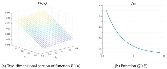
Figure 1. Two-dimensional section of the function P* and the function Q*.

6.2. Testing

Testing was performed using the data from the collection $\mathcal{T}$, which included the lake area $S\left[t\right]$, the average annual temperature $T\left[t\right]$, and the annual precipitation $R\left[t\right]$, $t=25,\cdots ,35$. An ensemble of trajectories of the model’s observed output $v\left[t\right]$ was generated using Monte Carlo simulations and sampling of the entropy-optimal PDFs $P^{*}\left(\mathbf{a}\right)$, $Q^{*}\xi$ on the testing interval. In addition, the trajectory of the empirical means $\overline{v}\left[t\right]$ and the dimensions of the empirical standard deviation area were calculated.

The quality of RME estimation was characterized by the absolute and relative errors:

$$\begin{array}{ccc}\hfill & & AbsErr=\sqrt{\sum _{t=26}^{35}{\left(S\left[t\right]-\overline{v}\left[t\right]\right)}^2}=0.3446,\hfill \end{array}$$

(39)

$$\begin{array}{ccc}& & RelErr=\frac{\sqrt{{\sum }_{t=26}^{35}{\left(S\left[t\right]-\overline{v}\left[t\right]\right)}^2}}{\sqrt{{\sum }_{t=26}^{35}{S}^2\left[t\right]}+\sqrt{{\sum }_{t=26}^{35}{\overline{v}}^2\left[t\right]}}=0.0089.\hfill \end{array}$$

(40)

The generated ensemble of the trajectories is shown in Figure 2.

Figure 2. Ensemble of the trajectories (gray domain), the standard deviation area (dark gray domain), the empirical mean trajectory, and the lake area data.

7. Discussion

Given an available data collection, the RME procedure allows estimation of the PDFs of a model’s random parameters under measurement noises corresponding to the maximum uncertainty (maximum entropy). In addition, this procedure needs no assumptions about the structure of the estimated PDFs or the statistical properties of the data and measurement noises.

An entropy-optimal model can be simulated by sampling the PDFs to generate an empirical ensemble of a model’s output trajectories and to calculate its empirical characteristics (the mean and median trajectories, the standard deviation area, interquartile sets, and others).

The RME procedure was illustrated with an example of the estimation of the parameters of a linear regression model for the evolution of the thermokarst lake area in Western Siberia. In this example, the procedure demonstrated a good estimation accuracy.

However, these positive features of the procedure were achieved with computational costs. Despite their analytical structure, the RME estimates of the PDFs depend on Lagrange multipliers, which are determined by solving the balance equations with the so-called integral components (the mathematical expectations of random parameters and measurement noises). Calculating the values of multidimensional integrals may require appropriate computing resources.

8. Conclusions

The problem of randomized maximum entropy estimation of a probability density function based on real available data has been formulated and solved. The developed estimation algorithm (the RME algorithm) finds the conditional maximum of an information entropy functional on a set of admissible probability density functions characterized by the empirical balance equations for Lagrange multipliers. These equations define an implicit dependence of the Lagrange multipliers on the data collection. The existence of such an implicit function for any values in a data collection has been established. The function’s behavior for a data collection of a greater size has been studied, and the asymptotic efficiency of the RME estimates has been proved.

The positive features of RME estimates have been illustrated with an example of estimation and testing a linear dynamic regression model of the evolution of the thermokarst lake area in Western Siberia with real data.

References

- Vapnik, V.N. Statistical Learning Theory; Wiley: New York, NY, USA, 1998. [Google Scholar]
- Witten, I.H.; Eibe, F. Data Mining: Practical Machine Learning Tools and Techniques; Morgan Kaufmann: Heidelberg, Germany, 2005. [Google Scholar]
- Bishop, C.M. Pattern Recognition and Machine Learning. Series: Information Theory and Statistics; Springer: New York, NY, USA, 2006. [Google Scholar]
- Hastie, T.; Tibshirani, R.; Friedman, J. The Elements of Statistical Learning; Springer: New York, NY, USA, 2001. [Google Scholar]
- Vorontsov, K.V. Mathematical Methods of Learning by Precedents: A Course of Lectures; Moscow Institute of Physics and Technology: Moscow, Russia, 2013. [Google Scholar]
- Goldberger, A.S. A Course in Econometrics; Harvard University Press: Cambridge, UK, 1991. [Google Scholar]
- Aivazyan, S.A.; Enyukov, I.S.; Meshalkin, L.D. Prikladnaya Statistika: Issledovanie Zavisimostei (Applied Statistics: Study of Dependencies); Finansy i Statistika: Moscow, Russia, 1985. [Google Scholar]
- Lagutin, M.B. Naglyadnaya Matematicheskaya Statistika (Visual Mathematical Statistics); BINOM, Laboratoriya Znanii: Moscow, Russia, 2013. [Google Scholar]
- Roussas, G. A Course of the Mathematical Statistics; Academic Press: San Diego, CA, USA, 2015. [Google Scholar]
- Malouf, R. A comparison of algorithms for maximum entropy parameters estimation. In Proceedings of the 6th Conference on Natural Language Learning 2002 (CoNLL-2002), Taipei, Taiwan, 31 August–1 September 2002; Volume 20, pp. 1–7. [Google Scholar]
- Borwein, J.; Choksi, R.; Marechal, P. Probability distribution of assets inferred from option prices via principle of maximum entropy. SIAM J. Optim. 2003, 14, 464–478. [Google Scholar] [CrossRef]
- Golan, A.; Judge, G.; Miller, D. Maximum Entropy Econometrics: Robust Estimation with Limited Data; John Wiley & Sons: New York, NY, USA, 1997. [Google Scholar]
- Golan, A. Information and Entropy econometrics—A review and synthesis. Found. Trends Econom. 2008, 2, 1–145. [Google Scholar] [CrossRef]
- Csiszar, I.; Matus, F. On minimization of entropy functionals under moment constraints. In Proceedings of the IEEE International Symposium on Information Theory, Toronto, ON, Canada, 6–11 July 2008. [Google Scholar]
- Loubes, J.-M. Approximate maximum entropy on the mean for instrumental variable regression. Stat. Probab. Lett. 2012, 82, 972–978. [Google Scholar] [CrossRef]
- Borwein, J.M.; Lewis, A.S. Partially-finite programming in L1 and existence of maximum entropy estimates. SIAM J. Optim. 1993, 3, 248–267. [Google Scholar] [CrossRef]
- Burg, J.P. The relationship between maximum entropy spectra and maximum likelihood spectra. Geophysics 1972, 37, 375–376. [Google Scholar] [CrossRef]
- Christakos, G. A Bayesian/maximum entropy view to the spatial estimation problem. Math. Geol. 1990, 22, 763–777. [Google Scholar] [CrossRef]
- Singh, V.P.; Guo, H. Parameter estimation for 3-parameter generalized Pareto distribution by the principle of maximum entropy. Hydrol. Sci. J. 1994, 40, 165–181. [Google Scholar] [CrossRef]
- Popkov, Y.S.; Dubnov, Y.A.; Popkov, A.Y. Randomized machine learning: Statement, solution, applications. In Proceedings of the 2016 IEEE 8th International Conference on Intelligent Systems (IS), Sofia, Bulgaria, 4–6 September 2016. [Google Scholar] [CrossRef]
- Popkov, A.Y.; Popkov, Y.S. New methods of entropy-robust estimation for randomized models under limited data. Entropy 2014, 16, 675–698. [Google Scholar] [CrossRef]
- Krasnosel’skii, M.A.; Vainikko, G.M.; Zabreyko, R.P.; Ruticki, Y.B.; Stet’senko, V.V. Approximate Solutions of Operator Equations; Wolters-Noordhoff Publishing: Groningen, The Netherlands, 1972. [Google Scholar] [CrossRef]
- Ioffe, A.D.; Tikhomirov, V.M. Theory of Extremal Problems; Elsevier: New York, NY, USA, 1974. [Google Scholar]
- Alekseev, V.M.; Tikhomirov, V.M.; Fomin, S.V. Optimal Control; Springer: Boston, MA, USA, 1987. [Google Scholar]
- Kaashoek, M.A.; van der Mee, C. Recent Advances in Operator Theory and Its Applications; Birkhäuser Basel: Basel, Switzerland, 2006. [Google Scholar]
- Kolmogorov, A.N.; Fomin, S.V. Elements of the Theory of Functions and Functional Analysis; Dover Publication: New York, NY, USA, 1999. [Google Scholar]
- Krasnoselskii, M.A.; Zabreiko, P.P. Geometrical Methods of Nonlinear Analysis; Springer: Berlin, Germany; New York, NY, USA, 1984. [Google Scholar]
- Gantmacher, F.R.; Brenner, J.L. Applications of the Theory of Matrices; Dover: New York, NY, USA, 2005. [Google Scholar]
- Riordan, B.; Verbula, D.; McGruire, A.D. Shrinking ponds in subarctic Alaska based on 1950–2002 remotely sensed images. J. Geophys. Res. 2006, 111, G04002. [Google Scholar] [CrossRef]
- Kirpotin, S.; Polishchuk, Y.; Bruksina, N. Abrupt changes of thermokarst lakes in Western Siberia: Impacts of climatic warming on permafrost melting. Int. J. Environ. Stud. 2009, 66, 423–431. [Google Scholar] [CrossRef]
- Western Siberia Thermokarsk Lakes Dataset. Available online: https://cloud.uriit.ru/index.php/s/0DOrxL9RmGqXsV0 (accessed on 20 February 2021).
Publisher’s Note: MDPI stays neutral with regard to jurisdictional claims in published maps and institutional affiliations. |
© 2021 by the author. Licensee MDPI, Basel, Switzerland. This article is an open access article distributed under the terms and conditions of the Creative Commons Attribution (CC BY) license (http://creativecommons.org/licenses/by/4.0/).