On the Similarity and Dependence of Time Series

Abstract

In this paper, we undertake the problem of evaluating interrelation among time series. Interrelation is measured using a similarity index. In this paper, we suggest a new one based on the known fuzzy transform (F-transform), which has been proven to remove higher frequencies than a given threshold and reduce the random noise significantly. The F-transform also provides an estimation of the slope of time series in a given imprecisely delineated time. We prove some of the suggested index properties and show its ability to measure similarity (and thus the interrelation) on a selection of several real financial time series. The method is well interpretable and easy to adjust.

1. Introduction

Time series form a topic of research that has been widely studied for many years (for some recent references, see [1,2,3,4,5]). In 2006, Yang and Wu [6] rated mining information from time series as one of the top ten challenging data mining problems due to its particular properties. One of its subareas is assessing similarity between time series, i.e., the degree to which a given time series resembles another one is the core of many tasks, such as retrieval and clustering, classification, and even forecasting [7].

Analysis of time series in theoretical and practical aspects is an crucial part of the study of stock markets. Empirical research started in 1933 [8] and was focused on the analysis of the stock market as a single independent time series, often referred to as a univariate time series analysis. The financial time series consists, in this case, of single observations recorded sequentially over equal time increments. However, in recent decades, worldwide economies have become increasingly related to each other. Various phenomena such as politics, social media platforms, and even pandemics can influence a set of financial time series similarly. Nowadays, there are likely to be groups of stocks that follow similar time-based patterns behavior simultaneously or with some time delay; Therefore, a crucial question is raised: “what are all the stocks that behave similarly to given stock A? ”. Nevertheless, devising a proper similarity measure to find a similar behavior among time series is a non-trivial task [3].

Besides Euclidean distance measures, many others can be found in the literature [9,10,11,12,13,14,15]. In 1999, Mantegna suggested a methodology known as the standard one adopted and followed by many researchers in different areas. As of 2020, his paper and his book, Ref. [16] have been cited several thousand times. To calculate the distance (similarity) among assets, Mantegna recommends the use of correlation among returns. Many researchers aim to improve his method concerning the clustering algorithm or the distance measure itself in continuation of his work. This can be briefly described as follows.

Let N be the number of assets, $P_i\left(t\right)$ be the price at time t of asset i, 1 ≤ i ≤ N, then the log-return of an asset $r_i\left(t\right)$, is calculated as follows:

$$r_i\left(t\right)=log{P}_i\left(t\right)-log{P}_i(t-1).$$

To determine the distance (similarity) between each pair $(i,j)$ of assets, he suggests to compute the correlation of returns and then correlation coefficients $\left(p_{ij}\right)$ into distance using the following equation:

$$d_{ij}=\sqrt{2(1-p_{ij})}.$$

He employs a minimum spanning tree (MST) to cluster the most similar assets in the form of a tree. A distinctive indexed hierarchy is another product of the resulting MST, corresponding to the one given by the dendrogram obtained using the single linkage clustering algorithm. However, there are few concerns regarding this standard methodology. The biggest problem is instability, which can be partially caused by the MST algorithm or by the correlation coefficient. Note that the correlation is not applied to the financial time series but to their returns; therefore, the price values’ dependence might be lost. Moreover, it is known that Pearson linear correlation is sensitive towards outliers and generally not suitable for other probability distributions except for the Gaussian one. It is also challenging to interpret linkage changes during the time since there is a high level of statistical uncertainty associated with the correlation estimation [17]. Interestingly, as one might expect, the higher the correlation coefficient between an asset pair, the more reliable their link should be. However, in [18], the authors show that this hypothesis is not always satisfied in practice. Mantegna [19] concludes that a better approach is needed to use a distance measure other than the expected square deviation and one that is distribution-free. Thus, researchers have investigated different measures of distance from specific viewpoints.

The similarity between two-time series should not be computed based on their values only but also based on the corresponding slopes. This is important specifically in the stock market because relative variations in the price values affect the trading performance. A positive slope indicates an uptrend, and a negative slope indicates a downtrend. However, a question is raised, how we can include the slopes. A possible and very reasonable solution is provided by the fuzzy transform (F-transform). Recall that we distinguish degrees of the F-transform: the zero-degree F-transform provides components giving information about the given function’s average values in a specified area. The first-degree F-transform provides an estimation of the tangent of the given function in a specified area.

This paper aims to suggest a new similarity index between two time series that combines both values of time series and their slopes. We prove some of its properties of this index and demonstrate its behavior on a selection of several real financial time series.

The structure of this paper is as follows. Section 2 is an overview of the main principles of the fuzzy transform and its properties. In Section 3, we introduce the new similarity index and prove some of its properties. In Section 4, we demonstrate our index on several financial time series.

2. Preliminaries

2.1. The Principle of F-Transform

The fuzzy (F-)transform is a universal approximation technique which was introduced by I. Perfilieva in [20,21]. Its fundamental idea consists in two steps:

(i)

Direct F-transform: Transform a bounded real continuous function $f:[a,b]\to \mathbb{R}$ to a finite vector $\mathbf{F}\left[f\right]$ of components. This is realized using a fuzzy partition which is a finite set of fuzzy sets distributed over the domain $[a,b]$.

(ii)

Inverse F-transform: Transform the vector $\mathbf{F}\left[f\right]$ back into a function $\widehat{f}$ that approximates the original function f.

The F-transform has the following properties:

• it is a universal approximator,
• it has ability to filter out high frequencies and to reduce noise [22],
• it provides estimation of average values of derivatives over an imprecisely specified area [23],
• its computational complexity is polynomial.

The parameters of the F-transform can be set in such a way that the approximating function $\widehat{f}$ has the desired properties.

These properties make the F-transform suitable for applications in various tasks when processing time series. More about F-transform and its applications can be found in [24].

2.1.1. Fuzzy Partition

Recall that by a fuzzy set, we understand a function $A:U\to [0,1]$ where U is a set (a universe) and $[0,1]$ is the interval of reals understood as a set of truth degrees. The element $A\left(u\right)\in [0,1]$ is called membership degree of $u\in U$ in the fuzzy set A. In general, it is a support of a certain algebra (cf. Section 2.3) whose operations induce operations with fuzzy sets ( We refer the reader to the extensive literature on fuzzy set theory and fuzzy logic, for example [24] and the citations therein). The support of a fuzzy set A is the set $\left(A\right)=\{u\in U\mid A(u)>0\}$.

The fundamental step of the F-transform procedure is forming a fuzzy partition of the domain $[a,b]$, which is a finite set of fuzzy sets

$$\mathcal{A}=\{A_0,\dots ,A_n\},n\ge 2,$$

(1)

defined over nodes $c_0,\dots ,c_n\in [a,b]$ such that

$$a=c_0,\dots ,c_n=b$$

(2)

and for each $k=0,\dots ,n$, $A_k\left(c_k\right)=1$. Furthermore, each fuzzy set $A_k$, $k=1,\dots ,n-1$, has the support $(c_{k-1},c_{k+1})$, which implies that $A_k\left(x\right)=0$ for all $x\in [a,c_{k-1}]\cup c_{k+1},b]$ (We formally put $c_{-1}=c_0=a$ and $c_{n+1}=c_n=b$). The fuzzy sets $A_k$ are often called basic functions. Note that $A_1,\dots ,A_{n-1}$ cover the whole domain $(a,b)$, i.e., $(a,b)={\bigcup }_{k=1}^{n-1}\mathrm{Supp}\left(A_k\right)$ (since $A_1\left(a\right)=A_{n-1}\left(b\right)=0$). For $k=0$ and $k=n$, we consider only halves of the functions $A_k$, i.e., $A_0$ has the support $(c_0,c_1)$ and $A_n$ the support $(c_{n-1},c_n)$. A typical h-uniform triangular fuzzy partition is depicted in Figure 1.

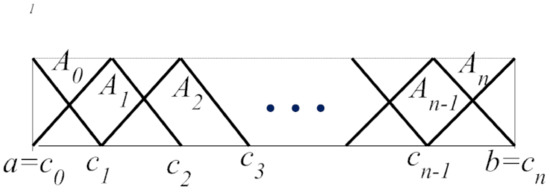
Figure 1. A typical h-uniform triangular fuzzy partition.

Remark 1.

In general, the fuzzy sets from $A_k\in \mathcal{A}$ must fulfill five axioms, namely: normality, locality (bounded support), continuity, unimodality, and orthogonality, where the latter is formally defined as ${\sum }_{i=0}^n{A}_i\left(x\right)=1$, $x\in [a,b]$. For precise formulation of these axioms see [20,24].

A fuzzy partition $\mathcal{A}$ is called h-uniform if the nodes $c_0,\dots ,c_n$ are h-equidistant, i.e., for all $k=0,\dots ,n-1$, $c_{k+1}=c_k+h$, where $h=(b-a)/n$ and the fuzzy sets $A_1,\dots ,A_{n-1}$ are shifted copies of a generating function $A:[-1,1]\to [0,1]$ such that for all $k=1,\dots ,n-1$

$$A_k\left(x\right)=A\left(\frac{x-c_k}{h}\right),x\in [c_{k-1},c_{k+1}].$$

2.1.2. Zero Degree Fuzzy Transform

After determining the fuzzy partition $A_0,\dots ,A_n\in \mathcal{A}$, we construct a direct F-transform of a continuous function f as a vector ${\mathbf{F}}^0\left[f\right]=(F_0^0\left[f\right],\dots ,F_n^0\left[f\right])$, where each k-th component$F_k^0\left[f\right]$ is equal to

$$F_k^0\left[f\right]=\frac{{\int }_a^{b}f\left(x\right)A_k\left(x\right)dx}{{\int }_a^b{A}_k\left(x\right)dx},k=0,\dots ,n.$$

(3)

One can see that each $F_k^0\left[f\right]$ component is a weighted average of the functional values $f\left(x\right)$, where weights are the membership degrees $A_k\left(x\right)$. The inverse F-transform of f with respect to ${\mathbf{F}}^0\left[f\right]$ is a continuous function $\widehat{f}:[a,b]\to \mathbb{R}$ such that

$$\widehat{f}\left(x\right)=\sum _{k=0}^n{F}_k^0\left[f\right]·A_k\left(x\right),x\in [a,b].$$

Theorem 1.

The inverse F-transform $\widehat{f}$ has the following properties:

 (a)

It coincides with f if the latter is a constant function.

 (b)

The sequence of inverse F-transforms $\left\{{\widehat{f}}_n\right\}$ determined by a sequence of uniform fuzzy partitions based on uniformly distributed nodes with $h=(b-a)/n$ uniformly converges to f for $n\to \infty$.

 (c)

The F-transform is linear, i.e., if $f\left(x\right)=\alpha u\left(x\right)+\beta v\left(x\right)$ then $\widehat{f}\left(x\right)=\alpha \widehat{u}\left(x\right)+\beta \widehat{v}\left(x\right)$ for all arguments x.

 (d)

Let $f\left(x\right)=q\in \mathbb{R}$ for all $x\in [a,b]$. Then, $F_k^0\left[f\right]=q$ for any $k=1,\dots ,n-1$.

All the details and full proofs can be found in [20,21].

2.1.3. Higher Degree Fuzzy Transform

The components $F_k^0\left[f\right]$ of the zero degree F-transform are real numbers (in the sequel, we will write F${}^0$-transform). If we replace $F_k^0\left[f\right]$ by polynomials of m-th degree, $m\ge 0$, we obtain a higher degree F-transform (F${}^m$ transform). A detailed description of this F-transform including full proofs of its properties can be found in [21]. It is important to note that the F${}^1$ transform enables us to also estimate derivatives of the given function f over a non-precisely specified area.

The direct $F^1$-transform of f with respect to $\mathcal{A}$ is a vector ${\mathbf{F}}^1\left[f\right]=(F_1^1\left[f\right]\left(x\right),\dots ,$$F_{n-1}^1\left[f\right]\left(x\right))$ linear functions

$$F_k^1\left[f\right]\left(x\right)={\beta }_k^0+{\beta }_k^1(x-c_k),k=0,\dots ,n$$

(4)

with the coefficients ${\beta }_k^0,{\beta }_k^1$ given by

$$\begin{array}{cc}\hfill {\beta }_k^0& =\frac{{\int }_{c_{k-1}}^{c_{k+1}}f\left(x\right)A_k\left(x\right)dx}{{\int }_{c_{k-1}}^{c_{k+1}}{A}_k\left(x\right)dx},\hfill \end{array}$$

(5)

$$\begin{array}{cc}\hfill {\beta }_k^1& =\frac{{\int }_{c_{k-1}}^{c_{k+1}}f\left(x\right)(x-c_k)A_k\left(x\right)dx}{{\int }_{c_{k-1}}^{c_{k+1}}{(x-c_k)}^2{A}_k\left(x\right)dx}.\hfill \end{array}$$

(6)

Note that ${\beta }_k^0=F_k^0\left[f\right]$, i.e., the coefficients ${\beta }_k^0$ are just the components $F_k^0\left[f\right]$ given in (3). The F${}^1$-transform enjoys the properties stated in Theorem 1 (see [21]). In comparison with the F${}^0$ transform, it is more precise. Let us remark that in general, we can define n-th degree F-transform. Of course, for higher n, it is more complex but also more precise. In practice, it is sufficient to consider only $n\in \{0,1,2\}$.

The following theorem is important for mining information from time series [24].

Theorem 2.

If f is four-times continuously differentiable on $[a,b]$, then for each $k=1,\dots ,n-1$,

$$\begin{array}{cc}\hfill {\beta }_k^0& =f\left(c_k\right)+O\left(h^2\right),\hfill \end{array}$$

(7)

$$\begin{array}{cc}\hfill {\beta }_k^1& =f^{\prime }\left(c_k\right)+O\left(h^2\right).\hfill \end{array}$$

(8)

Thus, each F${}^1$-transform component provides a weighted average of values of the function f in the area around the node $c_k$ (7), and also a weighted average of slopes (22) of f in the same area.

Lemma 1.

If $\mathcal{A}$ is an h-uniform fuzzy partition and each basic function $A_k\in \mathcal{A}$ has a triangular shape, then the following can be proved:

$$\begin{array}{cc}\hfill & {\int }_{c_{k-1}}^{c_{k+1}}{A}_k\left(x\right)dx=h,\hfill \end{array}$$

(9)

$$\begin{array}{cc}\hfill {\beta }_k^0& =\frac{1}{h}{\int }_{c_{k-1}}^{c_{k+1}}f\left(x\right)A_k\left(x\right)dx,\hfill \end{array}$$

(10)

$$\begin{array}{cc}\hfill {\beta }_k^1& =\frac{12}{h^3}{\int }_{c_{k-1}}^{c_{k+1}}f\left(x\right)(x-c_k)A_k\left(x\right)dx.\hfill \end{array}$$

(11)

Lemma 2.

Let $\mathcal{A}$ be an h-uniform fuzzy partition with triangular membership functions and let $\left|f\right(x\left)\right|\le 1$ for all $x\in [a,b]$. Then,

 (a)

$|{\beta }_k^0|\le 1$.

 (b)

If $h\ge 12$ then $|{\beta }_k^1|\le 1$.

Proof. 

(a) Using (10) we have:

$$|{\beta }_k^0|=\frac{1}{h}\left|{\int }_{c_{k-1}}^{c_{k+1}}f\left(x\right)A_k\left(x\right)dx\right|\le \frac{1}{h}{\int }_{c_{k-1}}^{c_{k+1}}\left|f\left(x\right)\right|A_k\left(x\right)dx\le \frac{1}{h}{\int }_{c_{k-1}}^{c_{k+1}}{A}_k\left(x\right)dx=\frac{h}{h}=1.$$

(b) Using (11) we have:

$$\begin{array}{c}|{\beta }_k^1|=\frac{12}{h^3}\left|{\int }_{c_{k-1}}^{c_{k+1}}f\left(x\right)(x-c_k)A_k\left(x\right)dx\right|\le \frac{12}{h^3}{\int }_{c_{k-1}}^{c_{k+1}}\left|f\left(x\right)\right||(x-c_k)|A_k\left(x\right)dx\le \hfill \\ \hfill \frac{12}{h^3}{\int }_{c_{k-1}}^{c_{k+1}}h{A}_k\left(x\right)dx=\frac{12}{h}\end{array}$$

 □

2.2. Time Series and F-Transform

A time series is a stochastic process (see [25,26])

$$X:\mathbb{T}\times \mathsf{\Omega }\to \mathbb{R}$$

where $\mathsf{\Omega }$ is a set of elementary random events and $\mathbb{T}=\{0,\dots ,p\}\subset \mathbb{N}$ is a finite set whose elements are interpreted as time moments. Statistical models assume that each $X\left(t\right)$, $t\in \mathbb{T}$ is a random variable having a specific distribution function.

Fuzzy techniques are based on the following decomposition model:

$$X(t,\omega )=\mathit{T}\mathit{C}\left(t\right)+S\left(t\right)+R(t,\omega ),t\in \mathbb{T},$$

(12)

where $\mathit{T}\mathit{C}\left(t\right)$ is a trend-cycle that can be further decomposed into trend and cycle, i.e., $\mathit{T}\mathit{C}\left(t\right)=\mathit{T}\mathit{r}\left(t\right)+C\left(t\right)$. The $S\left(t\right)$ is a seasonal component that is a mixture of r periodic functions

$$S\left(t\right)=\sum _{j=1}^r{P}_j{e}^{i{\lambda }_{j}t}$$

(13)

where ${\lambda }_1,\dots ,{\lambda }_r$ are frequencies and $P_j$, $j=1,\dots ,r$ are constants. Without loss of generality, we can assume that the frequencies are ordered ${\lambda }_1<\cdots <{\lambda }_r$.

Note that $\mathit{T}\mathit{C}$ and S are ordinary non-stochastic functions. Only R is a random noise, i.e., a stationary stochastic process such that the mean $\mathbf{E}\left(R\right(t,\omega \left)\right)=0$ and variance $\mathbf{Var}\left(R\right(t,\omega \left)\right)<\sigma$, $t\in \mathbb{T}$.

In practice, we always have only one realization of time series at disposal. Formally, this means that we fix $\omega \in \mathsf{\Omega }$. Then, we write

$$X=\left\{X\right(t)\mid t\in \mathbb{T}\}$$

(14)

and understand that X is an ordinary real (or complex) valued function.

Let us now assume that inside (14), the real time series is hidden

$$Z\left(t\right)=\mathit{T}\mathit{C}\left(t\right)+\sum _{j=1}^{r-s}{P}_j{e}^{i{\lambda }_{j}t}+R^{\prime }(t,\omega ),t\in \mathbb{T},$$

(15)

where $0<s<r$ and $R^{\prime }\le R$. In other words, we assume that the time series X is “spoiled” by some frequencies that are too high ${\lambda }_{r-s+1},\dots ,{\lambda }_r$ (they may correspond, e.g., to a certain unwelcome volatility) that are removed in Z.

The following theorem demonstrates the power of the F-transform for time series analysis.

Theorem 3.

Let $X\left(t\right)$ be realization of the stochastic process (4) and Z be its smoothed version (15). Let $\mathcal{A}$ be a fuzzy partition over the set of equidistant nodes (2) with the distance h. Let the fuzzy sets $A_k\in \mathcal{A}$ be N-times differentiable and put $d=h{\lambda }_{r-s}$.

 (a)

The corresponding inverse F-transform $\widehat{X}$ of $X\left(t\right)$ gives the following estimation of Z:

$$|\widehat{X}\left(t\right)-Z\left(t\right)|\le \omega (2h,Z)+O\left(d^{-N}\right)+\left|\widehat{R}\left(t\right)\right|$$

(16)

for $t\in \mathbb{T}$, where $\omega (2h,Z)$ is a modulus of continuity of Z w.r.t. 2 h (The modulus of continuity of a function $f:[a,b]\to$ w.r.t. h is $\omega (h,f)=max\left\{\right|f\left(x\right)-f\left(y\right)|\mid |x-y|<h,x,y\in [a,b\left]\right\}$).

 (b)

$\mathbf{E}\left(R\left(t\right)\right)=\mathbf{E}\left(\widehat{R}\left(t\right)\right)=0$ and $\mathbf{Var}\left(\widehat{R}\left(t\right)\right)\le \mathbf{Var}\left(R\left(t\right)\right)<\sigma$.

The details for the proof of this theorem can be found in [20,27,28,29]. The theorem holds both for the F${}^0$- as well as for F${}^1$-transform. It follows from this theorem that the F-transform filters out frequencies higher than a given threshold and reduces the noise R. In [27], it was even proved that if the correlation function of R has a quick decay, then ${lim}_{h\to \infty }\mathbf{Var}\left(\widehat{R}\left(t\right)\right)=0$.

Remark 2.

The fuzzy partition $\mathcal{A}$ is not constructed over the discrete set of natural numbers $\mathbb{T}=\{1,\dots ,p\}$ but over the interval of real numbers $[0,p]$.

It follows from Theorem 3 that $\widehat{X}\approx Z$; we can estimate the real time series Z with high fidelity. First, we set a proper fuzzy partition and and compute the F${}^0$-transform of $X\left(t\right)$:

$${\mathbf{F}}^0\left[X\right]=(F_0^0\left[X\right]\left(t\right),\dots ,F_n^0\left[X\right]\left(t\right)).$$

Then, we compute the inverse $\widehat{X}$, which approximates the real time series Z. According to [22], we should set

$$h=q\frac{2\pi }{{\lambda }_{r-s}}$$

(17)

for some natural number q (in practice, it is sufficient to put $q\in \{1,2\}$). The frequencies ${\lambda }_1,\dots ,{\lambda }_r$ can be found using the well known periodogram—see [25,26].

Remark 3.

The edge components $F_0\left[X\right],F_n\left[X\right]$ are distorted because only half of the corresponding basic functions are used. This problem can be solved in two ways: either we confine only to the complete components $F_k\left[X\right]$ for $k=1,\dots ,n-1$, or we artificially prolong $\mathbb{T}$ to the left and right by h and extrapolate the corresponding values $X\left(t_{-i}\right)=X\left(t_i\right)$ for $i=1,\dots ,h$, and similarly in the right side of $\mathbb{T}$.

2.3. Fuzzy Equality

Let $⟨[0,1],\vee ,\wedge ,\otimes ,\to ,0,1⟩$ be an algebra of truth values where $\vee =max$, $\wedge =min$, $a\otimes b=max\{0,a+b-1\}$, $a\to b=min\{1,1-a+b\}$, $a,b\in [0,1]$. This algebra is called Łukasiewicz standard algebra (Of course, there are also other algebras used as algebras of truth values for fuzzy set theory and fuzzy logic. However, the Łukasiewicz algebra, has a prominent position because of its good properties in many respects and, therefore, we confine our theory to it only). It serves us as the algebra of truth values. The operations with fuzzy sets are defined using the operations on it [30,31].

A binary fuzzy relation is a fuzzy set $R:U\times V\to [0,1]$. If $u\in U,v\in V$, then we often write the membership degree $R(u,v)$ of the couple $(u,v)$ in R as $\left(uRv\right)\in [0,1]$.

Definition 1.

Let $\doteq :U\times U\to [0,1]$ be a binary fuzzy relation.

 (i)

It is reflexive if $(u\doteq u)=1$ for all $u\in U$.

 (ii)

It is symmetric if $(u\doteq v)=(v\doteq u)$ for all $u,v\in U$.

 (iii)

It is transitive if $(u\doteq v)\otimes (v\doteq w)\le (u\doteq w)$ for all $u,v,w\in U$.

 (iv)

It is separated if for all $u,v\in U$

$$(u\doteq v)=1\hspace{1em}iff\hspace{1em}u=v$$

(fuzzy equality in the degree 1 reduces to the classical equality).

Definition 2.

 (i)

A binary fuzzy relation ≐ on U is a fuzzy symmetry if it is reflexive and transitive.

 (ii)

A fuzzy symmetry is a fuzzy equality if it is also transitive.

3. Similarity of Time Series

As already mentioned, there are many kinds of similarity indexes introduced. Most of them are based on the distance between the values of time series (cf., e.g., [2,32,33,34]). The problem is that all such indexes are necessarily distorted by random noise. Consequently, the real shape of time series is hidden. Solution of these difficulties can be given by the fuzzy transform.

Let us consider two time series $X,Y$ with the same time domain $\mathbb{T}$. Since the time series values can fall within very different ranges, we first normalize both time series to make their values comparable. The normalization will be done w.r.t. maximal values $\overline{X}=max\left\{\right|X\left(t\right)|\mid t\in \mathbb{T}\}$, $\overline{Y}=max\left\{\right|Y\left(t\right)|\mid t\in \mathbb{T}\}$. Then, we put

$$\begin{array}{cc}\hfill X^N& =\left\{\left.\frac{X\left(t\right)}{\overline{X}}\right|t\in \mathbb{T}\right\},\hfill \end{array}$$

(18)

$$\begin{array}{cc}\hfill Y^N& =\left\{\left.\frac{Y\left(t\right)}{\overline{Y}}\right|t\in \mathbb{T}\right\}.\hfill \end{array}$$

(19)

Let us choose two numbers $h_0,h_1>0$, compute $n_0=\frac{\left|\mathbb{T}\right|}{h_0}$ and $n_1=\frac{\left|\mathbb{T}\right|}{h_1}$ and form two $h_0$, $h_1$-uniform fuzzy partitions $\mathcal{A}$, $\mathcal{B}$ of the time domain $\mathbb{T}$.

Let us compute components of zero- and first-degree F-transforms of the time series (18) and (19):

$$\begin{array}{cccc}\hfill {\mathbf{F}}^0\left[X^N\right]& =(F_1^0\left[X^N\right]\left(t\right),\dots ,F_{n_0-1}^0\left[X^N\right]\left(t\right)),\hfill & \hfill {\mathbf{F}}^1\left[X^N\right]& =(F_1^1\left[X^N\right]\left(t\right),\dots ,F_{n_1-1}^1\left[X^N\right]\left(t\right))\hfill \end{array}$$

(20)

$$\begin{array}{cccc}\hfill {\mathbf{F}}^0\left[Y^N\right]& =(F_1^0\left[Y^N\right]\left(t\right),\dots ,F_{n_0-1}^0\left[Y^N\right]\left(t\right)),\hfill & \hfill {\mathbf{F}}^1\left[Y^N\right]& =(F_1^1\left[Y^N\right]\left(t\right),\dots ,F_{n_1-1}^1\left[Y^N\right]\left(t\right))\hfill \end{array}$$

(21)

where the zero-degree components are computed on the basis of the fuzzy partition $\mathcal{A}$, and the first-degree ones on the basis of $\mathcal{B}$. Note that in the direct F-transforms above, we omitted the first and the last components. For further processing, we need only the coefficients ${\beta }_k^0$, $k=1,\dots ,n_0-1$, and ${\beta }_k^1$, $k=1,\dots ,n_1-1$ defined in (5) and (6).

Based on that, we form to each time series $X^N,Y^N$, two new reduced time series, namely a time series of values and that of tangents:

$$\begin{array}{cc}\hfill {\mathbf{\beta }}_X^0& =\{{\beta }_{X,k}^0\mid k=1,\dots ,n_0-1\},\hfill \end{array}$$

(22)

$$\begin{array}{cc}\hfill {\mathbf{\beta }}_X^1& =\{{\beta }_{X,k}^1\mid k=1,\dots ,n_1-1\},\hfill \end{array}$$

(23)

$$\begin{array}{cc}\hfill {\mathbf{\beta }}_Y^0& =\{{\beta }_{Y,k}^0\mid k=1,\dots ,n_0-1\},\hfill \end{array}$$

(24)

$$\begin{array}{cc}\hfill {\mathbf{\beta }}_Y^1& =\{{\beta }_{Y,k}^1\mid k=1,\dots ,n_1-1\}.\hfill \end{array}$$

(25)

Hence, ${\mathbf{\beta }}_X^0$ and ${\mathbf{\beta }}_Y^0$ are time series of average values of the respective time series $X^N,Y^N$ over the imprecisely specified areas $A_k\in \mathcal{A}$, $k=1,\dots ,n-1$, and ${\mathbf{\beta }}_X^1$ and ${\mathbf{\beta }}_Y^1$ are time series of average values of tangents of the time series $X^N,Y^N$ over the imprecisely specified areas $B_k\in \mathcal{B}$, $k=1,\dots ,n-1$.

Definition 3.

Let $X,Y$ be time series (14). Then the index of similarity of two time series is the number

$$S(X,Y)=max\left\{0,1-\frac{{\kappa }_0}{n_0-1}\sum _{k=1}^{n_0-1}|{\beta }_{X,k}^0-{\beta }_{Y,k}^0|+\frac{{\kappa }_1}{n_1-1}\sum _{k=1}^{n_1-1}\frac{|{\beta }_{X,k}^1-{\beta }_{Y,k}^1|}{\phi }\right\}$$

(26)

where φ is a common normalization factor assuring that both $|{\beta }_{X,k}^1|,|{\beta }_{Y,k}^1|\le 1$ for all $k=1,\dots ,n_1-1$ and ${\kappa }_0,{\kappa }_1$ are sensitivity constants.

The suggested similarity index thus considers not only distances between average values of time series but also distances between average values of tangents in the same areas. The constants ${\kappa }_0,{\kappa }_1$ increase or decrease sensitivity of values and slopes of the compared time series. Clearly, if ${\kappa }_0>1$ then $S(X,Y)$ is more sensitive to differences between the corresponding values of $X,Y$, while ${\kappa }_1>1$ does the same for their slopes.

The normalization factor $\phi$ can be specified, e.g., as follows. Let $X,Y,Z$ be time series (14) and put

$$\begin{array}{cc}\hfill \overline{{\beta }_X^1}& =max\left\{\right|{\beta }_{X,k}^1|\mid k=1,\dots ,n_1-1\},\hfill \\ \hfill \overline{{\beta }_Y^1}& =max\left\{\right|{\beta }_{Y,k}^1|\mid k=1,\dots ,n_1-1\},\hfill \\ \hfill \overline{{\beta }_Z^1}& =max\left\{\right|{\beta }_{Z,k}^1|\mid k=1,\dots ,n_1-1\}.\hfill \end{array}$$

Then,

$$\phi =max\{\overline{{\beta }_X^1},\overline{{\beta }_Y^1}\}$$

(27)

is a normalization factor common for $X,Y$ and

$$\phi =max\{\overline{{\beta }_X^1},\overline{{\beta }_Y^1},\overline{{\beta }_Z^1}\}$$

(28)

is a normalization factor common for $X,Y,Z$.

The following is immediate.

Lemma 3.

$$S(X,Y)\in [0,1].$$

Theorem 4.

Let $X,Y$ be time series (14).

 (a)

The similarity index $S(X,Y)$ is a separated fuzzy symmetry.

 (b)

If $S(X,Y)\ne 0$ then, the transitivity property $S(X,Z)\otimes S(Z,Y)\le S(X,Y)$ holds for any time series Z.

Proof. 

(a) If $X=Y$ then, obviously, $S(X,Y)=1$. The symmetry follows immediately from the properties of absolute value.

(b) Let $\phi$ be a common normalization factor for $X,Y,Z$. After rewriting, we obtain

$$\begin{array}{c}max\left\{0,1-\frac{{\kappa }_0}{n_0-1}\sum _{k=1}^{n_0-1}|{\beta }_{X,k}^0-{\beta }_{Y,k}^0|+\frac{{\kappa }_1}{n_1-1}\sum _{k=1}^{n_1-1}\frac{|{\beta }_{X,k}^1-{\beta }_{Y,k}^1|}{\phi }+1-\frac{{\kappa }_0}{n_0-1}\sum _{k=1}^{n_0-1}|{\beta }_{Y,k}^0-{\beta }_{Z,k}^0|\right.+\hfill \\ \hfill \left.\frac{{\kappa }_1}{n_1-1}\sum _{k=1}^{n_1-1}\frac{|{\beta }_{Y,k}^1-{\beta }_{Z,k}^1|}{\phi }-1\right\}\le 1-\frac{{\kappa }_0}{n_0-1}\sum _{k=1}^{n_0-1}|{\beta }_{X,k}^0-{\beta }_{Z,k}^0|+\frac{{\kappa }_1}{n_1-1}\sum _{k=1}^{n_1-1}\frac{|{\beta }_{X,k}^1-{\beta }_{Z,k}^1|}{\phi }.\end{array}$$

If the left-hand side is equal to 0, then the inequality is trivially fulfilled. By the assumption, we have to verify that

$$\begin{array}{cc}\hfill \sum _{k=1}^{n_0-1}|{\beta }_{X,k}^0-{\beta }_{Z,k}^0|& \le \sum _{k=1}^{n_0-1}|{\beta }_{X,k}^0-{\beta }_{Y,k}^0|+\sum _{k=1}^{n_0-1}|{\beta }_{Y,k}^0-{\beta }_{Z,k}^0|,\hfill \\ \hfill \sum _{k=1}^{n_1-1}\frac{|{\beta }_{X,k}^1-{\beta }_{Z,k}^1|}{\phi }& \le \sum _{k=1}^{n_1-1}\frac{|{\beta }_{X,k}^1-{\beta }_{Y,k}^1|}{\phi }+\sum _{k=1}^{n_1-1}\frac{|{\beta }_{Y,k}^1-{\beta }_{Z,k}^1|}{\phi }\hfill \end{array}$$

which holds using the triangular inequality and the properties of ordered groups.

Finally, let $S(X,Y)=1$. Then, it follows from (26) that ${\beta }_{X,k}^0={\beta }_{Y,k}^0$ for all $k=1,\dots ,n_0-1$, as well as ${\beta }_{X,k}^1={\beta }_{Y,k}^1$ for all $k=1,\dots ,n_1-1$. Since all the fuzzy sets $A_1,\dots ,A_{n_0-1}$ as well as $B_1,\dots ,B_{n_1-1}$ cover the whole time domain $\mathbb{T}$, we conclude that $X=Y$.  □

Proposition 1.

Let $X\equiv q_1$ and $X\equiv q_2$ be two constant time series. Then,

$$S(X,Y)=1.$$

Proof. 

It follows from (18) and (19) that $X^N=Y^N\equiv 1$. Then, ${\beta }_{X,k}^0={\beta }_{Y,k}^0=1$ by Theorem 1(d), and ${\beta }_{X,k}^1={\beta }_{Y,k}^1=0$ by the properties of tangent.  □

It follows from this proposition that if both time series $X,Y$ are constant then they are fully similar.

4. Demonstration

In this section, we will apply the similarity index (26) to real data. In all cases, we used F${}^0$-transform with $h=3$ and the sensitivity constant ${\kappa }_0=2.5$, and F${}^1$-transform with $h=5$ and the sensitivity constant ${\kappa }_2=2$. These parameters were estimated according to the expert opinion based on practical experience. Setting $h=3$ is determined so as to not harm the real course of the time series too much, since longer h leads to greater smoothing. Similarly, $h=5$ is determined by the idea that the slope should be evaluated over a larger area since otherwise, it can be non-convincing. The parameters ${\kappa }_1,{\kappa }_2$ are estimated by testing the behavior of the index. The conditions for the setting of all four parameters are still a topic of further investigation.

For demonstration, we are inspired by a study [35]. In this paper, Junior et al. provide a view of which indices are the strongest influencers between 83 international market indices. Their results suggest that France and Germany were among the top index to send out the information to other markets. Based on the correlation dependency, the Czech Republic was among the top information receivers. Therefore, we chose these international stock exchange indices with the Russian market as a sample for demonstration. The data contain daily adjusting closing prices for 2016 ( Four international stock exchange indices, namely, Prague (PX), Paris (FCHI), Frankfurt (GDAXI), and Moscow (MOEX), were obtained from Yahoo finance). Several exciting events, such as the falling of oil prices and the Brexit announcement and voting, heavily affected the stock market in 2016 and its interrelations. Therefore, it is valuable to investigate the underlying relations. Figure 2 demonstrates the daily closing price of the above-mentioned four markets. Due to different national holidays, each market contains some missing values, which were omitted for similarity measurement.

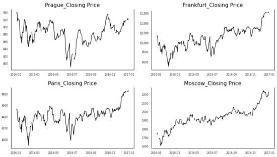
Figure 2. Closing price of four stocks.

Using the suggested similarity index, we evaluate pairwise similarities between the stocks and compare them with the known correlation coefficients based on rank correlations, namely Spearman, Kendall and Hoeffing D. The results are summarized in Table 1.

Table 1. Comparison of the similarity index with the known statistical correlation coefficients.

X Y	Prague Moscow	Prague Paris	Prague Frankfurt	B Frankfurt	Prague Moscow Distorted	Prague Prague Inverted
S(X, Y)	0.77	0.9	0.84	0.93	0	0.34
ineSpearman	0.16	0.6	0.33	0.86	0.04	−1
Kendall	0.12	0.42	0.23	0.69	0.04	−1
Hoeffding D	0.01	0.11	0.03	0.36	−0.002	1

The results reveal several interesting relations. The most similar stock to Prague is the Paris market, while Moscow has the lowest similarity. Another exciting relation is with regard to the Frankfurt market. The pair (Paris–Frankfurt) has a higher similarity in comparison with (Prague–Frankfurt). These relations are also visible in Figure 2. In Figure 3, Figure 4, Figure 5 and Figure 6, we demonstrate the behavior of the normalized prices for the mentioned similarity indices.

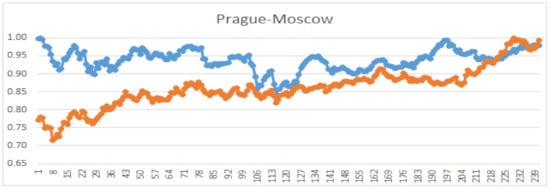
Figure 3. Comparison of graphs of normalized prices for Prague and Moscow; $S(\mathrm{Prague},\mathrm{Moscow})=0.77$.

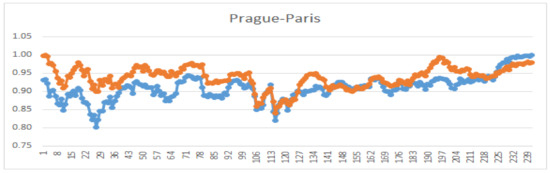
Figure 4. Comparison of graphs of normalized prices for Prague and Paris; $S(\mathrm{Prague},\mathrm{Paris})=0.9$.

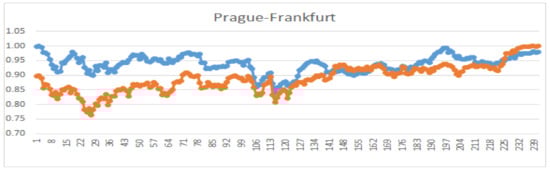
Figure 5. Comparison of graphs of normalized prices for Frankfurt and Prague; $S(\mathrm{Prague},\mathrm{Frankfurt})=0.84$.

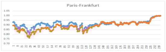
Figure 6. Comparison of graphs of normalized prices for Frankfurt and Paris; $S(\mathrm{Paris},\mathrm{Frankfurt})=0.93$.

To see whether the similarity index (26) reacts on very dissimilar time series, we artificially distorted the Moscow market and also artificially inverted the Prague market’s price values. The comparison (Prague–Moscow distorted) and (Prague–Prague inverted) is in Figure 7 and Figure 8. As one expects, there is zero similarity between Prague and distorted Moscow. However, the similarity between Prague and its inverted version remained non-zero, which is caused mainly by the found similarities between their corresponding slopes.

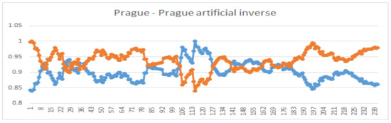
Figure 7. Comparison of graphs of Prague and its artificial inverse stock prices; $S(\mathrm{Prague},\mathrm{Prague}\mathrm{inverse})=0.34$.

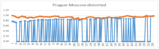
Figure 8. Comparison of graphs of Prague and artificially distorted Moscow stock prices; $S$(Prague,Moscow−distorted) = 0.

The rank correlation coefficients are a measure of a monotonic relationship. We chose them because they are less sensitive to outliers. Hoeffding’s D correlation is a measure of a non-linear and non-monotonous relationship. Note, that the sign of the Hoeffding’s D coefficient has no interpretation.

If the Spearman (and Kendall) coefficient is close to 0 and the Hoeffding coefficient is high, then the relationship is probably non-monotonic and non-linear. In our case, this did not happen. According to the statistical tests, all the correlation coefficients are non-zero (the p-values are practically zero) if the similarity index (26) is high. In the case $S$(Prague,Moscow−distorted) = 0, the correlation coefficients are statistically zero. However, when comparing (Prague–Prague inverted), the statistical tests show negative dependence, while $S(\mathrm{Prague},\mathrm{Prague}\mathrm{artificial}\mathrm{inverse})=0.34$. This is correct because the correlation coefficients measure dependence, while (26) measures similarity. The slopes of both time series have opposite signs and so, they decrease the value of the similarity (26). However, when inspecting Figure 7, one can see similarity in values of both time series and, therefore, the index still has non-zero value.

5. Conclusions

In this paper, we developed a new method for measuring similarity between time series. The method is based on the application of the fuzzy transform. The index compares F${}^0$-transform and F${}^1$-transform components. While the former measures similarity between time series values after the highest frequencies were removed and noise reduced, the former measures similarity between slopes of time series in short local periods.

We demonstrated the application of our index to four real financial time series and two artificial ones. Experimental results confirm its ability to measure the similarity between time series.

Further work will focus on the extension of the method to time series of various lengths. Another direction is to judge the evolution of the similarity throughout the years. We also plan to extend this idea to measuring dependence between time series.

References

- Mining, W.I.D. Data mining: Concepts and techniques. Morgan Kaufinann 2006, 10, 559–569. [Google Scholar]
- Keogh, E.; Kasetty, S. On the need for time series data mining benchmarks: A survey and empirical demonstration. Data Min. Knowl. Discov. 2003, 7, 349–371. [Google Scholar] [CrossRef]
- Fu, T.C. A review on time series data mining. Eng. Appl. Artif. Intell. 2011, 24, 164–181. [Google Scholar] [CrossRef]
- Liao, T.W. Clustering of time series data—A survey. Pattern Recognit. 2005, 38, 1857–1874. [Google Scholar] [CrossRef]
- Han, J.; Pei, J.; Kamber, M. Data Mining: Concepts and Techniques; Elsevier: Amsterdam, The Netherlands, 2011. [Google Scholar]
- Yang, Q.; Wu, X. 10 challenging problems in data mining research. Int. J. Inf. Technol. Decis. Mak. 2006, 5, 597–604. [Google Scholar] [CrossRef]
- Serra, J.; Arcos, J.L. An empirical evaluation of similarity measures for time series classification. Knowl.-Based Syst. 2014, 67, 305–314. [Google Scholar] [CrossRef]
- Mills, T.C.; Markellos, R.N. The Econometric Modelling of Financial Time Series; Cambridge University Press: Cambridge, UK, 2008. [Google Scholar]
- Goldin, D.Q.; Kanellakis, P.C. On similarity queries for time-series data: Constraint specification and implementation. In Proceedings of the International Conference on Principles and Practice of Constraint Programming, Cassis, France, 19–22 September 1995; Springer: Berlin/Heidelberg, Germany, 1995; pp. 137–153. [Google Scholar]
- Agrawal, R.; Faloutsos, C.; Swami, A. Efficient similarity search in sequence databases. In Proceedings of the International Conference on Foundations of Data Organization and Algorithms, Chicago, IL, USA, 13–15 October 1995; Springer: Berlin/Heidelberg, Germany, 1993; pp. 69–84. [Google Scholar]
- Berndt, D.J.; Clifford, J. Using dynamic time warping to find patterns in time series. In Proceedings of the KDD Workshop, Seattle, WA, USA, 31 July–1 August 1994; Volume 10, pp. 359–370. [Google Scholar]
- Ozsoyoglu, T.B.N.Y.M. Matching and indexing sequences of different lengths. In Proceedings of the Sixth International Conference on Information and Knowledge Management: CIKM’97, Las Vegas, NV, USA, 10–14 November 1997; Volume 6, p. 128. [Google Scholar]
- Alcock, R.J.; Manolopoulos, Y. Time-series similarity queries employing a feature-based approach. In Proceedings of the 7th Hellenic Conference on Informatics, Ioannina, Greece, 26–29 August 1999; pp. 27–29. [Google Scholar]
- Ruspini, E.H.; Zwir, I.S. Automated qualitative description of measurements. In Proceedings of the 16th IEEE Instrumentation and Measurement Technology Conference (Cat. No. 99CH36309), IMTC/99, Venice, Italy, 24–26 May 1999; Volume 2, pp. 1086–1091. [Google Scholar]
- Morrill, J.P. Distributed recognition of patterns in time series data: From sensors to informed decisions. Commun. ACM 1998, 41, 45–52. [Google Scholar] [CrossRef]
- Mantegna, R.N.; Stanley, H.E. Introduction to Econophysics: Correlations and Complexity in Finance; Cambridge University Press: Cambridge, UK, 1999. [Google Scholar]
- Marti, G.; Nielsen, F.; Bińkowski, M.; Donnat, P. A review of two decades of correlations, hierarchies, networks and clustering in financial markets. arXiv 2017, arXiv:1703.00485. [Google Scholar]
- Tumminello, M.; Coronnello, C.; Lillo, F.; Micciche, S.; Mantegna, R.N. Spanning trees and bootstrap reliability estimation in correlation-based networks. Int. J. Bifurc. Chaos 2007, 17, 2319–2329. [Google Scholar] [CrossRef]
- Mantegna, R.N. Hierarchical structure in financial markets. Eur. Phys. J. B-Condens. Matter Complex Syst. 1999, 11, 193–197. [Google Scholar] [CrossRef]
- Perfilieva, I. Fuzzy Transforms: Theory and applications. Fuzzy Sets Syst. 2006, 157, 993–1023. [Google Scholar] [CrossRef]
- Perfilieva, I.; Daňková, M.; Bede, B. Towards a Higher Degree F-transform. Fuzzy Sets Syst. 2011, 180, 3–19. [Google Scholar] [CrossRef]
- Novák, V.; Perfilieva, I.; Holčapek, M.; Kreinovich, V. Filtering out high frequencies in time series using F-transform. Inf. Sci. 2014, 274, 192–209. [Google Scholar] [CrossRef]
- Kreinovich, V.; Perfilieva, I. Fuzzy Transforms of Higher Order Approximate Derivatives: A Theorem. Fuzzy Sets Syst. 2011, 180, 55–68. [Google Scholar]
- Novák, V.; Perfilieva, I.; Dvořák, A. Insight into Fuzzy Modeling; Wiley & Sons: Hoboken, NJ, USA, 2016. [Google Scholar]
- Anděl, J. Statistical Analysis of Time Series; SNTL: Praha, Czech Republic, 1976. (In Czech) [Google Scholar]
- Hamilton, J. Time Series Analysis; Princeton University Press: Princeton, NJ, USA, 1994. [Google Scholar]
- Nguyen, L.; Holčapek, M. Higher Degree Fuzzy Transform: Application to Stationary Processes and Noise Reduction. In Advances in Fuzzy Logic and Technology 2017; Kacprzyk, J., Szmidt, E., Zadrożny, S., Atanassov, K., Krawczak, M., Eds.; Springer: Berlin/Heidelberg, Germany, 2018; Volume 3, pp. 1–12. [Google Scholar]
- Nguyen, L.; Holčapek, M. Suppression of High Frequencies in Time Series Using Fuzzy Transform of Higher Degree. In Information Processing and Management of Uncertainty in Knowledge-Based Systems: 16th International Conference, IPMU 2016; Carvalho, J., Lesot, M.J., Kaymak, U., Vieira, S., Bouchon-Meunier, B., Yager, R., Eds.; Springer: Berlin/Heidelberg, Germany, 2016; Volume 2, pp. 705–716. [Google Scholar]
- Nguyen, L.; Novák, V. Filtering out high frequencies in time series using F-transform with respect to raised cosine generalized uniform fuzzy partition. In Proceedings of the International Conference FUZZ-IEEE 2015, Istanbul, Turkey, 2–5 August 2015. [Google Scholar]
- Gottwald, S. Fuzzy Sets and Fuzzy Logic. The Foundations of Application—From a Mathematical Point of View; Vieweg: Braunschweig/Wiesbaden, Germany; Teknea: Toulouse, France, 1993. [Google Scholar]
- Novák, V.; Perfilieva, I.; Močkoř, J. Mathematical Principles of Fuzzy Logic; Kluwer: Boston, MA, USA, 1999. [Google Scholar]
- Keogh, E.; Wei, L.; Xi, X.; Lee, S.-H.; Vlachos, M. LB-Keogh Supports Exact Indexing of Shapes Under Rotation Invariance With Arbitrary Representations and Distance Measures. In Proceedings of the 32nd International Conference on Very Large Data Bases, Seoul, Korea, 12–15 September 2006. [Google Scholar]
- Wang, X.; Mueen, A.; Ding, H.; Trajcevski, G.; Scheuermann, P.; Keogh, E. Experimental comparison of representation methods and distance measures for time series data. Data Min. Knowl. Discov. 2013, 26, 275–309. [Google Scholar] [CrossRef]
- Yeh, C.M.; Zhu, Y.; Ulanova, L.; Begum, N.; Ding, Y.; Dau, H.A.; Silva, D.F.; Mueen, A.; Keogh, E. Matrix Profile I: All Pairs Similarity Joins for Time Series: A Unifying View That Includes Motifs, Discords and Shapelets. In Proceedings of the 2016 IEEE 16th International Conference on Data Mining (ICDM), Barcelona, Spain, 12–15 December 2016. [Google Scholar]
- Junior, L.S.; Mullokandov, A.; Kenett, D.Y. Dependency relations among international stock market indices. J. Risk Financ. Manag. 2015, 8, 227–265. [Google Scholar] [CrossRef]
Publisher’s Note: MDPI stays neutral with regard to jurisdictional claims in published maps and institutional affiliations. |
© 2021 by the authors. Licensee MDPI, Basel, Switzerland. This article is an open access article distributed under the terms and conditions of the Creative Commons Attribution (CC BY) license (http://creativecommons.org/licenses/by/4.0/).