A High-Dimensional Counterpart for the Ridge Estimator in Multicollinear Situations

Abstract

The ridge regression estimator is a commonly used procedure to deal with multicollinear data. This paper proposes an estimation procedure for high-dimensional multicollinear data that can be alternatively used. This usage gives a continuous estimate, including the ridge estimator as a particular case. We study its asymptotic performance for the growing dimension, i.e., $p\to \infty$ when n is fixed. Under some mild regularity conditions, we prove the proposed estimator’s consistency and derive its asymptotic properties. Some Monte Carlo simulation experiments are executed in their performance, and the implementation is considered to analyze a high-dimensional genetic dataset.

1. Introduction

Consider the multiple regression model given by

$$\mathbf{Y}=\mathbf{X}\mathit{\beta }+\mathit{ϵ},$$

(1)

where $\mathbf{Y}={(y_1,\dots ,y_n)}^{\top }$ is a vector of n responses, $\mathbf{X}={({\mathbf{x}}_1,\dots ,{\mathbf{x}}_n)}^{\top }$ is an $n\times p$ design matrix, with the ith predictor ${\mathbf{x}}_i\in {\mathbb{R}}^p$, $\mathit{\beta }={({\mathit{\beta }}_1,\dots ,{\mathit{\beta }}_p)}^{\top }$ is the coefficients vector, and $\mathit{ϵ}$ is an n-vector of unobserved errors. Further, we shall assume $\mathbb{E}\left(\mathit{ϵ}\right)=\mathbf{0}$, $\mathbb{E}\left(\mathit{ϵ}{\mathit{ϵ}}^{\top }\right)={\sigma }^2{\mathbf{I}}_n$, ${\sigma }^2>0$.

When $p<n$, the ordinary least squares (LS) estimator of $\mathit{\beta }$ is given by

$$\begin{array}{ccc}\hfill \widehat{\mathit{\beta }}& =& \underset{\mathit{\beta }\in {\mathbb{R}}^p}{\arg \min }\mathcal{S}\left(\mathit{\beta }\right),\mathcal{S}\left(\mathit{\beta }\right)={(\mathbf{Y}-\mathbf{X}\mathit{\beta })}^{\top }(\mathbf{Y}-\mathbf{X}\mathit{\beta })\hfill \\ & =\hfill & {\left({\mathbf{X}}^{\top }\mathbf{X}\right)}^{-1}{\mathbf{X}}^{\top }\mathbf{Y}.\hfill \end{array}$$

(2)

However, for the high dimensional (HD) case, $p>n$ the LS estimator cannot be obtained, because ${\mathbf{X}}^{\top }\mathbf{X}$ is rank deficient. It is well known that the ridge regression (RR) estimator of [1], followed by [2] regularization, however, exists. The rationale is to add a positive value $k>0$ to the eigenvalues of ${\mathbf{X}}^{\top }\mathbf{X}$ to efficiently estimate the parameters via ${\widehat{\mathit{\beta }}}^{\mathrm{Ridge}}={({\mathbf{X}}^{\top }\mathbf{X}+k{\mathbf{I}}_p)}^{-1}{\mathbf{X}}^{\top }\mathbf{Y}$. Refer to Saleh et al. [3] for theory and application of the RR approach. Using the projection of $\mathit{\beta }$ onto the row space of $\mathbf{X}$ is a well-described remedy. Wang et al. [4] used this technique and proposed a high dimensional LS estimator as a limiting case of the RR, while Buhlmann [5] also used the projection method and developed a bias correction in the RR estimator to propose a bias-corrected RR estimator for the high dimensional setting. Shao and Deng [6] used the method and proposed to threshold the RR estimator when the projection vector is sparse, in the sense that many of its components are small and demonstrated consistency. Dicker [7] studied the minimum property of the RR estimator and derived its asymptotic risk for the growing dimension, i.e., $p\to \infty$. Although the RR estimator involves high dimensional problems, there exits a counterpart that has not been considered in high dimension.

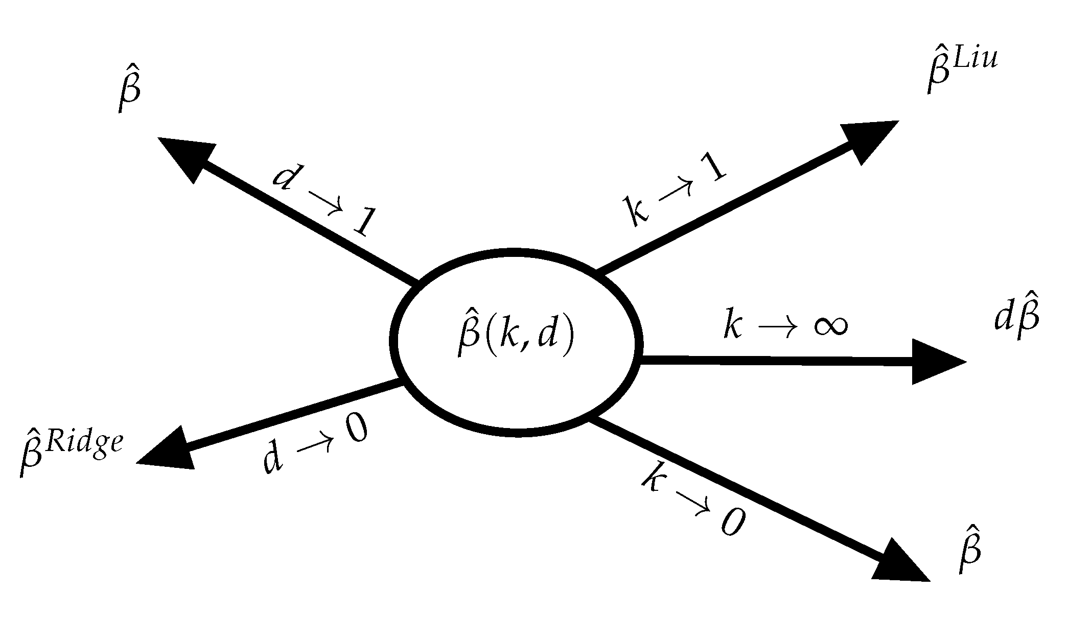
An Existing Two-Parameter Biased Estimator

It is well known that the RR estimator is an efficient approach for multicollinear situations. Since then, many authors have developed ridge-type estimators to overcome the issue of multicollinearity. One drawback of the RR estimator is that it is a non-linear function of the tuning parameter. Hence, Liu [8] developed a similar estimator; however, it is linear for the tuning parameter via the following optimization problem, for the case $p<n$:

$$\underset{\mathit{\beta }\in {\mathbb{R}}^p}{min}\mathcal{S}\left(\mathit{\beta }\right)+{(d\widehat{\mathit{\beta }}-\mathit{\beta })}^{\top }(d\widehat{\mathit{\beta }}-\mathit{\beta }).$$

(3)

The solution to the optimization problem (3) has the form

$${\widehat{\mathit{\beta }}}^{\mathrm{Liu}}={({\mathbf{X}}^{\top }\mathbf{X}+{\mathbf{I}}_p)}^{-1}({\mathbf{X}}^{\top }\mathbf{Y}+d\widehat{\mathit{\beta }}),$$

(4)

where $d\in (0,1)$ is termed as the biasing parameter.

Combining the advantages of the RR and Liu estimators, Ozkale and Kaciranlar [9] proposed a two-parameter estimator by solving the following optimization problem:

$$\underset{\mathit{\beta }\in {\mathbb{R}}^p}{min}\mathcal{S}\left(\mathit{\beta }\right)+k\left[{(d\widehat{\mathit{\beta }}-\mathit{\beta })}^{\top }(d\widehat{\mathit{\beta }}-\mathit{\beta })-c\right],$$

(5)

where c is a constant, and k is the Lagrangian multiplier. The resulting two-parameter ridge estimator has the form

$$\begin{array}{c}\hfill \widehat{\mathit{\beta }}(k,d)={({\mathbf{X}}^{\top }\mathbf{X}+k{\mathbf{I}}_p)}^{-1}({\mathbf{X}}^{\top }\mathbf{Y}+kd\widehat{\mathit{\beta }})\end{array}$$

(6)

The above estimator has several advantages and can be simplified to LS, RR, and Liu estimators as limiting cases (see Figure 1). It can be argued that this estimator can also be interpreted as a restricted estimator under stochastic prior information about $\mathit{\beta }$.

Figure 1. Special limiting cases.

With growing dimensions p, $p>n$, the LS estimator (2) cannot be obtained, so it is not possible to use the two-parameter ridge estimator in Equation (6). Hence, developing a high-dimensional two-parameter version of this estimator and studying its asymptotic performance is interesting and worthwhile. Therefore, in this paper, we propose a high-dimensional version of Ozkale and Kaciranlar’s estimator and give the asymptotic properties. The paper’s organization is as follows: In Section 2, a high-dimensional two-parameter estimator is proposed, and its asymptotic characteristics are discussed. Section 3 indicates the generalized cross validation for choosing the parameters. In Section 4, some simulation experiments are presented to assess the novel estimator’s statistical and computational performance, and an application to the AML data is illustrated in this section The conclusion is presented in the last section.

2. The Proposed Estimator

In this section, we develop an HD estimator and establish its asymptotic properties. To show a component is dependent to p, we shall use the subscript p and particularly consider the scenarios in which $p\to \infty$ and n is fixed. This is termed large p, fixed n, which is more general than scenarios with $p/n\to \rho \in (0,\infty )$, a common assumption in high-dimensional settings.

Consider a diverging number of variables case, in which p is allowed to tend to infinity. This case fulfills the high-dimensional case $p>n$. Under this setting, the inverse of ${\mathbf{X}}^{\top }\mathbf{X}$ does not exist; however, the RR estimator is still valid and applicable. Further, the Liu estimator cannot be obtained. As a remedy, one can use the Moore–Penrose inverse of ${\mathbf{X}}^{\top }\mathbf{X}$, a particular case of the generalized inverse. Wang and Leng [10] showed that ${\left({\mathbf{X}}^{\top }\mathbf{X}\right)}^{-1}{\mathbf{X}}^{\top }$ can be seen as the Moore-Penrose inverse of $\mathbf{X}$ for $p<n$, and that ${\mathbf{X}}^{\top }{\left(\mathbf{X}{\mathbf{X}}^{\top }\right)}^{-1}$ is the Moore–Penrose inverse of $\mathbf{X}$ when $p>n$. This gives, for any $p,n>0$,

$$\begin{array}{c}\hfill {({\mathbf{X}}^{\top }\mathbf{X}+s{\mathbf{I}}_p)}^{-1}{\mathbf{X}}^{\top }={\mathbf{X}}^{\top }{(\mathbf{X}{\mathbf{X}}^{\top }+s{\mathbf{I}}_n)}^{-1},\end{array}$$

(7)

where s is an arbitrary nonegative constant.

Multiplying both sides of (7) by $\mathbf{Y}$ reveals that the LS estimator can be represented as

$$\begin{array}{ccc}\hfill \widehat{\mathit{\beta }}& =& \underset{s\to \infty }{lim}{({\mathbf{X}}^{\top }\mathbf{X}+s{\mathbf{I}}_p)}^{-1}{\mathbf{X}}^{\top }\mathbf{Y}\hfill \\ & =\hfill & \underset{s\to \infty }{lim}{\mathbf{X}}^{\top }{(\mathbf{X}{\mathbf{X}}^{\top }+s{\mathbf{I}}_n)}^{-1}\mathbf{Y}\hfill \\ & =\hfill & {\mathbf{X}}^{\top }{\left(\mathbf{X}{\mathbf{X}}^{\top }\right)}^{-1}\mathbf{Y}.\hfill \end{array}$$

(8)

Now, for the HD case, substitute (8) in (6) to obtain

$$\begin{array}{ccc}\hfill {\widehat{\mathit{\beta }}}^{\mathrm{HD}}& =& {({\mathbf{X}}^{\top }\mathbf{X}+k_p{\mathbf{I}}_p)}^{-1}({\mathbf{X}}^{\top }\mathbf{Y}+k_p{d}_p{\mathbf{X}}^{\top }{\left(\mathbf{X}{\mathbf{X}}^{\top }\right)}^{-1}\mathbf{Y})\hfill \\ & =\hfill & {({\mathbf{X}}^{\top }\mathbf{X}+k_p{\mathbf{I}}_p)}^{-1}({\mathbf{X}}^{\top }+k_p{d}_p{\mathbf{X}}^{\top }{\left(\mathbf{X}{\mathbf{X}}^{\top }\right)}^{-1})\mathbf{Y}\hfill \\ & =\hfill & {({\mathbf{X}}^{\top }\mathbf{X}+k_p{\mathbf{I}}_p)}^{-1}({\mathbf{X}}^{\top }+k_p{d}_p{\mathbf{X}}^{+})\mathbf{Y},\hfill \end{array}$$

(9)

where ${\mathbf{X}}^{+}={\mathbf{X}}^{\top }{\left(\mathbf{X}{\mathbf{X}}^{\top }\right)}^{-1}$ is the Moore–Penrose inverse of $\mathbf{X}$.

We impose the following regularity conditions for studying the asymptotic performance of the estimator. ${\widehat{\mathit{\beta }}}^{\mathrm{HD}}$ given by (9).

(A1) 

$1/k_p=o\left(1\right)$. There exists a constant $0\le \delta <0.5$, such that a component of $\mathbf{X}$ is $O\left(k_p^{\delta }\right)$.

(A2) 

$d_p=o\left(1\right)$. There exists a constant $0\le \eta <0.5$, such that a component of ${\mathbf{X}}^{+}$ is $O\left(d_p^{-\eta }\right)$.

(A3) 

For sufficiently large p, there is a vector ${\mathbf{b}}_{p\times 1}$, such that $\mathit{\beta }={\mathbf{X}}^{\top }\mathbf{X}\mathbf{b}$, and there exists a constant $\epsilon >0$, such that each component of the vector ${\mathbf{b}}_{p\times 1}$ is $O(1/p^{\epsilon +1.5})$, and $k_p=o\left(p^{\epsilon }{a}_p\right)$, with $a_p=o\left(1\right)$. (An example of such choice is $k_p=\sqrt{p}$ and $\epsilon =0.5+\delta$).

(A4) 

For sufficiently large p, there exists a constant $\delta >0$, such that each component of $\mathit{\beta }$ is $O\left(p^{-2-\delta }\right)$ and $1/d_p=o\left(p^{\delta }\right)$. Further, $k_p^{\delta -1}=o\left(d_p\right)$.

Assumption (A3) is adopted from Luo [11]. Let ${\widehat{\mathit{\beta }}}^{\mathrm{HD}}={\left({\widehat{\mathit{\beta }}}_1^{\mathrm{HD}},\dots ,{\widehat{\mathit{\beta }}}_p^{\mathrm{HD}}\right)}^{\top }$.

Theorem 1. 

Assume(A1)and(A2). Then, $\mathrm{var}\left({\widehat{\mathit{\beta }}}_i^{\mathrm{HD}}\right)=o\left(1\right)$ for all $i=1,\dots ,p$.

Proof. 

For the proof, refer to Appendix A. □

Theorem 2. 

Assume(A1)–(A3). Further, suppose ${\lambda }_{ip}=O\left(k_p\right)$, where ${\lambda }_{ip}>0$ is the ith eigenvalue of ${\mathbf{X}}^{\top }\mathbf{X}$. Then, $bias\left({\widehat{\mathit{\beta }}}_i^{\mathrm{HD}}\right)=o\left(1\right)$ for all $i=1,2,\dots ,p$.

Proof. 

For the proof, refer to Appendix A. □

Using Theorems 1 and 2, it can be verified that the HD estimator ${\widehat{\mathit{\beta }}}^{\mathrm{HD}}$ is a consistent estimator for $\mathit{\beta }$ as $p\to \infty$.

The following result reveals the asymptotic distribution of this estimator as $p\to \infty$.

Theorem 3. 

Assume $1/k_p=o\left(1\right)$, and for sufficiently large p, there exists a constant $\delta >0$, such that each component of β is $O\left(1/p^{2+\delta }\right)$. Let $k_p=o\left(p^{\delta }\right)$, ${\lambda }_{ip}=o\left(k_p\right)$. Furthermore, suppose that $\mathit{ϵ}\sim {\mathcal{N}}_n\left(0,{\sigma }^2{\mathbf{I}}_n\right)$, ${\sigma }^2>0$. Then,

$$\frac{1}{d_p}\left({\widehat{\mathit{\beta }}}^{\mathrm{HD}}-\mathit{\beta }\right)\stackrel{\mathcal{D}}{\to }\mathcal{N}\left(\mathbf{0},{\sigma }^2{\mathbf{X}}^{+}{{\mathbf{X}}^{+}}^{\top }\right)asp\to \infty .$$

(10)

Proof. 

For the proof, refer to Appendix A. □

3. Generalized cross Validation

As noted, the estimator ${\widehat{\mathit{\beta }}}^{\mathrm{HD}}$ depends on both the ridge parameter $k_p$ and Liu parameter $d_p$ that must be optimized in practice. To do this, we use the generalized cross-validation (GCV) criterion. The GCV uses to choose the ridge and Liu parameters by minimizing an estimate of the unobservable risk function

$$\begin{array}{ccc}\hfill \mathrm{R}\left(\mathit{\beta };{\widehat{\mathit{\beta }}}^{\mathrm{HD}}\right)& =& \frac{1}{n}{\left(\mathrm{E}\left(\mathbf{Y}\right)-{\widehat{\mathbf{Y}}}^{\mathrm{HD}}(k_p,d_p)\right)}^{\top }\left(\mathrm{E}\left(\mathbf{Y}\right)-{\widehat{\mathbf{Y}}}^{\mathrm{HD}}(k_p,d_p)\right)\hfill \\ & =& \frac{1}{n}{∥\mathrm{E}\left(\mathbf{Y}\right)-\mathbf{X}{\widehat{\mathit{\beta }}}^{\mathrm{HD}}(k_p,d_p)∥}^2,\hfill \end{array}$$

where

$$\begin{array}{ccc}\hfill {\widehat{\mathbf{Y}}}^{\mathrm{HD}}(k_p,d_p)& =& \mathbf{X}{\widehat{\mathit{\beta }}}^{\mathrm{HD}}\hfill \\ & =& {({\mathbf{X}}^{\top }\mathbf{X}+k_p{\mathbf{I}}_p)}^{-1}({\mathbf{X}}^{\top }+k_p{d}_p{\mathbf{X}}^{+})\mathbf{Y}\hfill \\ & =& \mathbf{H}(k_p,d_p)\mathbf{Y},\hfill \end{array}$$

(11)

with $\mathbf{H}(k_p,d_p)=\mathbf{X}{({\mathbf{X}}^{\top }\mathbf{X}+k_p{\mathbf{I}}_p)}^{-1}({\mathbf{X}}^{\top }+k_p{d}_p{\mathbf{X}}^{+})$, termed as the hat matrix of $\mathbf{Y}$.

This is straightforward to demonstrate, as in [12].

$$\begin{array}{ccc}\hfill \mathrm{E}\left(\mathrm{R}\left(\mathit{\beta };{\widehat{\mathit{\beta }}}^{\mathrm{HD}}\right)\right)& =& \frac{1}{n}\parallel \left({\mathbf{I}}_n-\mathbf{H}(k_p,d_p)\right)\mathbf{X}\mathit{\beta }{\parallel }^2+\frac{{\sigma }^2}{n}\mathrm{tr}\left(\mathbf{H}{(k_p,d_p)}^{\top }\mathbf{H}(k_p,d_p)\right)\hfill \\ & =& {\nu }_1^2(k_p,d_p)+{\sigma }^2{\nu }_2(k_p,d_p),\hfill \end{array}$$

where ${\nu }_1^2(k_p,d_p)=\frac{1}{n}\parallel \left({\mathbf{I}}_n-\mathbf{H}(k,d)\right)\mathbf{X}\mathit{\beta }{\parallel }^2$ and ${\nu }_2(k_p,d_p)=\frac{1}{n}\mathrm{tr}\left(\mathbf{H}{(k_p,d_p)}^{\top }\mathbf{H}(k_p,d_p\right)$.

The GCV function is then defined as

$$\begin{array}{ccc}\hfill \mathrm{GCV}\left({\widehat{\mathit{\beta }}}^{\mathrm{HD}}\right)& =& \frac{\frac{1}{n}\parallel \left({\mathbf{I}}_n-\mathbf{H}(k_p,d_p)\right)\mathbf{y}{\parallel }^2}{{\left(1-\frac{1}{n}\mathrm{tr}\left(\mathbf{H}(k_p,d_p)\right)\right)}^2}\hfill \\ & =& \frac{\frac{1}{n}\parallel \left({\mathbf{I}}_n-\mathbf{H}(k_p,d_p)\right)\mathbf{y}{\parallel }^2}{{\left(1-{\mu }_1(k_p,d_p)\right)}^2},\hfill \end{array}$$

(12)

where ${\mu }_1(k_p,d_p)=\frac{1}{n}\mathrm{tr}\left(\mathbf{H}(k_p,d_p)\right)$.

The following theorem extends the GCV theorem proposed by Akdeniz and Roozbeh [13].

Theorem 4. 

According to the definition of GCV, we have

$$\begin{array}{ccc}\hfill \frac{\mathrm{E}\left(\mathrm{R}\left(\mathit{\beta };{\widehat{\mathit{\beta }}}^{\mathrm{HD}}\right)\right)-\mathrm{E}\left(\mathrm{GCV}\left({\widehat{\mathit{\beta }}}^{\mathrm{HD}}\right)\right)+{\sigma }^2}{\mathrm{E}\left(\mathrm{R}\left(\mathit{\beta };{\widehat{\mathit{\beta }}}^{\mathrm{HD}}\right)\right)}& =& \left(1-\frac{{\sigma }^2}{{\left(1-{\mu }_1(k_p,d_p)\right)}^2}\right)\hfill \\ & & +\frac{1}{D(k,d)}\times \frac{{\sigma }^2{\mu }_1{(k_p,d_p)}^2}{{\left(1-{\mu }_1(k_p,d_p)\right)}^2},\hfill \end{array}$$

where $D(k,d)={\nu }_1^2(k_p,d_p)+{\sigma }^2{\nu }_2(k_p,d_p)$, and consequently,

$$\begin{array}{ccc}\hfill \frac{\left|\mathrm{E}\left(\mathrm{R}\left(\mathit{\beta };{\widehat{\mathit{\beta }}}^{\mathrm{HD}}\right)\right)-\mathrm{E}\left(\mathrm{GCV}\left({\widehat{\mathit{\beta }}}^{\mathrm{HD}}\right)\right)+{\sigma }^2\right|}{\mathrm{E}\left(\mathrm{R}\left(\mathit{\beta };{\widehat{\mathit{\beta }}}^{\mathrm{HD}}\right)\right)}& <& \frac{{\sigma }^2}{{\left(1-{\mu }_1(k_p,d_p)\right)}^2}\hfill \\ & & \times \left(2{\mu }_1(k_p,d_p)+\frac{{\mu }_1{(k_p,d_p)}^2}{{\nu }_2(k_p,d_p)}\right),\hfill \end{array}$$

whenever $0<{\mu }_1(k_p,d_p)<1$.

Proof. 

r For the proof, refer to Appendix A. □

4. Numerical Investigations

In this section, for performance assessment of the proposed HD estimator ${\widehat{\mathit{\beta }}}^{\mathrm{HD}}$, we conduct a simulation study along with the analysis of real data.

4.1. Simulation

Here, we consider the multiple regression model with varying squared multiple correlation coefficient $R^2$ and error distribution, given by the following relation:

$$\mathbf{Y}=c\mathbf{X}\mathit{\beta }+\sigma \mathit{ϵ},$$

where $\mathit{\beta }={({\mathit{\beta }}_1,\mathbf{0})}^{\top }$, ${\mathit{\beta }}_1$ is the active set, and its dimension is $p_1=0.4p$. The absolute values of a normal distribution with mean 0 and standard deviation 5 is considered ${\mathit{\beta }}_1$. The remaining $p-p_1$ components are zero.

In this example, motivated by McDonald and Galarneau [14], the explanatory variables are computed by

$${\mathbf{x}}_j=\sqrt{1-{\rho }^2}{\mathbf{z}}_j+\rho {\mathbf{z}}_{p_1},j=1,\dots ,p,$$

where the ${\mathbf{z}}_j$s are independent standard normal pseudo-random vectors, and $\rho$ is specified such that the correlation between any two explanatory variables is given by ${\rho }^2$. Similarly to Zhu et al. [15], the variance is set to ${\sigma }^2=6.83$, and two different kinds of error distribution are taken for $\mathit{ϵ}$: (1) the standard normal is ${\mathcal{N}}_n(\mathbf{0},{\mathbf{I}}_n)$, and (2) standard t with 5 degrees of freedom $t_n(\mathbf{0},{\mathbf{I}}_n,5)$. The constant c is also varied to control the signal-to-noise ratio, and it is set to $0.5$, 1, and 2 with the corresponding $R^2=20\%,50\%\mathrm{and}80\%$. $R^2$ represents the proportion of the variable for a dependent variable that is explained by an independent variable or variables in a regression model.

We consider $\rho \in \{0.8,0.95\}$; the sample size and the number of covariates are set to $n\in \{30,50,100\}$, $p\in \{256,512,1024\}$, respectively. Following regularity conditions ($\mathbf{A}\mathbf{1}$)–($\mathbf{A}\mathbf{4}$), we set $k_p=\sqrt{p}$. For $\delta =0.25=1/4$, we take $d_p=p^{-1/5}$, which guarantees ($\mathbf{A}\mathbf{4}$). We then simulate ${\widehat{\mathit{\beta }}}^{\mathrm{HD}}$ and ${\widehat{\mathit{\beta }}}^{\mathrm{Ridge}}$ 100 times using Equation (9) and ${\widehat{\mathit{\beta }}}^{\mathrm{Ridge}}={({\mathbf{X}}^{\top }\mathbf{X}+k_p{\mathbf{I}}_p)}^{-1}{\mathbf{X}}^{\top }\mathbf{Y}$.

For comparison purposes, the quadratic bias (QB) and mean squared error (MSE) are computed according to

$$\mathrm{QB}\left({\widehat{\mathit{\beta }}}^{*}\right)=\frac{1}{100}\sum _{j=1}^{100}{({\widehat{\mathit{\beta }}}_j^{*}-\mathit{\beta })}^{\top }({\widehat{\mathit{\beta }}}_j^{*}-\mathit{\beta }),\mathrm{and}\mathrm{MSE}\left({\widehat{\mathit{\beta }}}^{*}\right)=\frac{1}{100}\sum _{j=1}^{100}{({\widehat{\mathit{\beta }}}_j^{*}-\mathit{\beta })}^{\top }({\widehat{\mathit{\beta }}}_j^{*}-\mathit{\beta }),$$

respectively, where ${\widehat{\mathit{\beta }}}^{*}$ is one of ${\widehat{\mathit{\beta }}}^{\mathrm{HD}}$ or ${\widehat{\mathit{\beta }}}^{\mathrm{Ridge}}$.

4.2. Review of Results

In Theorem 2, the condition for which the proposed ${\widehat{\mathit{\beta }}}^{\mathrm{HD}}$ is unbiased is investigated based on the eigenvalues of ${\mathbf{X}}^{\top }\mathbf{X}$. Here, we numerically analyze the biasedness of this estimator by comparing the ridge estimator concerning the parameters of the model. For this purpose, the difference in QB is reported in Table 1 by evaluating

$$\mathrm{diff}=\mathrm{QB}\left({\widehat{\mathit{\beta }}}^{\mathrm{HD}}\right)-\mathrm{QB}\left({\widehat{\mathit{\beta }}}^{\mathrm{Ridge}}\right).$$

Table 1. The difference between quadratic biases of the high dimensional and ridge estimators.

			$\mathit{\rho }=0.8$		$\mathit{\rho }=0.95$
			$\mathcal{N}(\mathbf{0},{\mathbf{I}}_{\mathit{n}})$	${\mathit{t}}_{\mathit{n}}(\mathbf{0},{\mathbf{I}}_{\mathit{n}},\mathbf{5})$	$\mathcal{N}(\mathbf{0},{\mathbf{I}}_{\mathit{n}})$	${\mathit{t}}_{\mathit{n}}(\mathbf{0},{\mathbf{I}}_{\mathit{n}},\mathbf{5})$
$\mathit{p}$	$\mathit{c}$	$\mathit{n}$	diff	diff	diff	diff
256	$0.5$	30	5.7657	5.7643	10.0535	10.1134
		50	6.4911	6.4941	11.4722	11.5088
		100	17.8314	17.8493	30.1008	30.4137
	1	30	22.9671	487.4169	39.6556	459.3473
		50	25.8621	522.6298	45.1138	480.5501
		100	70.8693	798.6551	118.1326	676.1919
	2	30	91.7526	2413.9746	158.0026	2256.1664
		50	103.3996	2587.7382	179.8509	2357.4111
		100	283.0549	3922.0057	470.4114	3259.2211
512	$0.5$	30	3.1943	3.2012	6.5528	6.6001
		50	4.4800	4.4781	9.5861	9.6151
		100	10.2121	10.2489	20.1828	20.3366
	1	30	12.7657	926.7540	26.0911	916.2663
		50	17.8861	1009.3595	38.0549	969.4353
		100	40.7254	1192.4455	79.9094	1095.9628
	2	30	51.0605	4621.0862	104.2892	4555.0569
		50	71.5157	5029.3107	151.9461	4809.2595
		100	162.7616	5920.6337	318.7343	5397.7878
1024	$0.5$	30	1.7594	1.7584	3.7384	3.7410
		50	3.9188	3.9345	9.2523	9.3437
		100	5.1236	5.1189	12.6469	12.6455
	1	30	7.0318	1637.6798	14.8960	1636.5664
		50	15.6758	1804.8548	36.9649	1763.7468
		100	20.4564	1940.6091	50.2993	1856.0197
	2	30	28.1221	8181.4255	59.5312	8167.9835
		50	62.7157	9008.4246	147.8715	8781.1968
		100	81.7756	9682.7404	147.8715	9229.7803

If diff is positive, then the quadratic bias of the proposed estimator is larger than that of the ridge estimator.

To comprise the MSEs, we use the relative mean square error (RMSE) given by

$$\mathrm{RMSE}=\frac{\mathrm{MSE}\left({\widehat{\mathit{\beta }}}^{\mathrm{Ridge}}\right)}{\mathrm{MSE}\left({\widehat{\mathit{\beta }}}^{\mathrm{HD}}\right)}.$$

The results are reported in Table 2. If $\mathrm{RMSE}>1$, then the proposed estimator has a smaller MSE compared to the ridge.

Table 2. The relative MSE of the high dimensional and ridge estimators.

			$\mathit{\rho }=0.8$		$\mathit{\rho }=0.95$
			$\mathcal{N}(\mathbf{0},{\mathbf{I}}_{\mathit{n}})$	${\mathit{t}}_{\mathit{n}}(\mathbf{0},{\mathbf{I}}_{\mathit{n}},\mathbf{5})$	$\mathcal{N}(\mathbf{0},{\mathbf{I}}_{\mathit{n}})$	${\mathit{t}}_{\mathit{n}}(\mathbf{0},{\mathbf{I}}_{\mathit{n}},\mathbf{5})$
$\mathit{p}$	$\mathit{c}$	$\mathit{n}$	RMSE	RMSE	RMSE	RMSE
256	$0.5$	30	1.0050	1.0050	1.0140	1.0139
		50	1.0058	1.0058	1.0161	1.0160
		100	1.0222	1.0222	1.0543	1.0539
	1	30	1.0032	1.0032	1.0179	1.0178
		50	1.0039	1.0039	1.0209	1.0209
		100	1.0221	1.0220	1.0883	1.0876
	2	30	0.9816	0.9816	0.9852	0.9851
		50	0.9793	0.9793	0.9829	0.9829
		100	0.9434	0.9435	0.9587	0.9584
512	$0.5$	30	1.0011	1.0011	1.0031	1.0031
		50	1.0016	1.0016	1.0048	1.0048
		100	1.0041	1.0041	1.0119	1.0119
	1	30	1.0004	1.0004	1.0029	1.0029
		50	1.0007	1.0007	1.0048	1.0048
		100	1.0023	1.0023	1.0139	1.0139
	2	30	0.9948	0.9948	0.9924	0.9924
		50	0.9929	0.9929	0.9895	0.9895
		100	0.9843	0.9843	0.9810	0.9809
1024	$0.5$	30	1.0003	1.0003	1.0009	1.0009
		50	1.0007	1.0007	1.0022	1.0022
		100	1.0009	1.0009	1.0031	1.0031
	1	30	1.0001	1.0001	1.0006	1.0006
		50	1.0002	1.0002	1.0017	1.0017
		100	1.0003	1.0003	1.0025	1.0025
	2	30	0.9984	0.9984	0.9973	0.9973
		50	0.9964	0.9964	0.9933	0.9933
		100	0.9954	0.9954	0.9910	0.9911

Based on the results of Table 1 and Table 2, the following conclusions are made:

(1)

The performance of the estimators is affected by the number of observations (n), the number of variables (p), the signal to noise ratio (c), and the degree of multicollinearity ($\rho$).

(2)

By increasing the degree of multicollinearity, $\rho$, although for both cases of error distributions, the QB of the proposed estimator increases for $c=0.5$ and 1, its MSE decreases dramatically since the RMSE increases.

(3)

The signal-to-noise shows the effect of $\mathit{\beta }$ in the model. Lower values (less than 1) are a sign of model sparsity, since, when c is small, the proposed estimator performs better than the ridge. This is evidence that our estimator is a better candidate as an alternative in sparse models in the MSE sense. However, the QB increases for large c values, which forces the model to overestimate the parameters.

(4)

As p increases, although the proposed estimator is superior to the ridge in sparse models (small c values), the efficiency decreases. This is more evident when the ratio $p/n$ becomes larger. This fact may come as poor performance of the proposed estimators, but our estimator is still preferred in high dimensions for sparse models.

(5)

Obviously, as n increases, so does the RMSE; however, the QB becomes very large, and it is due to the nature of the proposed estimators because of its complicated form. It must be noted that this does not contradict the results of Theorem 2, since the simulation scheme does not obey the regularity condition.

(6)

There is evidence of robustness for the distribution tail for sparse models, i.e., the QB and RMSE are the same for both normal and t distributions. However, as c increases, the QB of the proposed estimator explodes for the heavier tail distribution. This may be seen as a disadvantage of the proposed estimators, but even for large values of c, the RMSE stays the same, evidence of relatively small variance for the heavier tail distribution.

4.3. AML Data Analysis

This section assesses the performance of the proposed estimators using the mean prediction error (MPE) and MSE criteria of a data set adopted from Metzeler et al. [16], in which the information for 79 patients was collected. The data can be accessed from the Gene Expression Omnibus (GEO) data repository (http://www.ncbi.nlm.nih.gov/geo/ (accessed on 1 January 2021)) by the National Center for Biotechnology Information (NCBI), where the data is available under GEO accession number GSE12417. We only use the data set that was used as a test set. This contains gene expression data for 79 adult patients with cytogenetically normal acute myeloid leukemia (CN-AML), showing heterogeneous treatment outcomes. According to Sill et al. [17], we reduce the total number of 54,675 gene expression features that have been measured with the Affymetrix HG-U133 Plus 2.0 microarray technology to the top $p\in \{1000,2000\}$ features with the largest variance across all 79 samples. We considered overall survival time based on month as the response variable. The condition number of the design matrix for the AML data set is approximately $1095.80$, evident of severe multicollinearity among columns of the design matrix ([18], see p. 298). To find the optimum values of k and d, denoted by $k_{\mathrm{opt}}$ and $d_{\mathrm{opt}}$ for practical purposes, we use the GCV given by Equation (12). Hence, we use the following formulas:

$$\begin{array}{ccc}\hfill {\widehat{\mathit{\beta }}}^{\mathrm{HD*}}& =& {({\mathbf{X}}^{\top }\mathbf{X}+k_{\mathrm{opt}}{\mathbf{I}}_p)}^{-1}({\mathbf{X}}^{\top }\mathbf{Y}+k_{\mathrm{opt}}{d}_{\mathrm{opt}}{\mathbf{X}}^{\top }{\left(\mathbf{X}{\mathbf{X}}^{\top }\right)}^{-1}\mathbf{Y})\hfill \\ \hfill {\widehat{\mathit{\beta }}}^{\mathrm{Ridge*}}& =& {({\mathbf{X}}^{\top }\mathbf{X}+k_{\mathrm{opt}}{\mathbf{I}}_p)}^{-1}{\mathbf{X}}^{\top }\mathbf{Y}.\hfill \end{array}$$

To compute the MPE and MSE, we divide the whole data set into two train ($\mathcal{T}=({\mathbf{X}}^{\mathrm{train}},{\mathbf{Y}}^{\mathrm{trian}})$) and validation ($\mathcal{V}=({\mathbf{X}}^{\mathrm{valid}},{\mathbf{Y}}^{\mathrm{valid}})$) sets, comprising $70\%$ and $30\%$, respectively. Then, the measures are evaluated using

$$\begin{array}{ccc}\hfill {\mathrm{MPE}}_{\mathrm{boot}}\left({\widehat{\mathit{\beta }}}^{*}\right)& =& \frac{1}{\mathrm{N}.\mathrm{boot}}\sum _{j=1}^{\mathrm{N}.\mathrm{boot}}{({\mathbf{X}}^{\mathrm{valid}}{\widehat{\mathit{\beta }}}_j^{\mathrm{train}*}-{\mathbf{Y}}^{\mathrm{valid}})}^{\top }({\mathbf{X}}^{\mathrm{valid}}{\widehat{\mathit{\beta }}}_j^{\mathrm{train}*}-{\mathbf{Y}}^{\mathrm{valid}}),\hfill \\ \hfill {\mathrm{MSE}}_{\mathrm{boot}}\left({\widehat{\mathit{\beta }}}^{*}\right)& =& \frac{1}{\mathrm{N}.\mathrm{boot}}\sum _{j=1}^{\mathrm{N}.\mathrm{boot}}{({\widehat{\mathit{\beta }}}_j^{\mathrm{train}*}-{\mathit{\beta }}^{\mathrm{HD}*})}^{\top }({\widehat{\mathit{\beta }}}_j^{\mathrm{train}*}-{\mathit{\beta }}^{\mathrm{HD}*}),\hfill \end{array}$$

where $\mathrm{N}.\mathrm{boot}$ stands for the number of bootstrapped sample, ${\widehat{\mathit{\beta }}}^{*}$ is one of the proposed and ridge estimators, and ${\widehat{\mathit{\beta }}}^{\mathrm{HD}*}$ is the assumed true parameter obtained by Equation (9) from the whole data set.

$$\begin{array}{c}\hfill {\mathrm{RMPE}}_{\mathrm{boot}}=\frac{{\mathrm{MPE}}_{\mathrm{boot}}\left({\widehat{\mathit{\beta }}}^{\mathrm{Ridge}*}\right)}{{\mathrm{MPE}}_{\mathrm{boot}}\left({\widehat{\mathit{\beta }}}^{\mathrm{HD}*}\right)}{\mathrm{RMSE}}_{\mathrm{boot}}=\frac{{\mathrm{MSE}}_{\mathrm{boot}}\left({\widehat{\mathit{\beta }}}^{\mathrm{Ridge}*}\right)}{{\mathrm{MSE}}_{\mathrm{boot}}\left({\widehat{\mathit{\beta }}}^{\mathrm{HD}*}\right)}\end{array}$$

The results are tabulated in Table 3 for the number of bootstrap $\mathrm{N}.\mathrm{boot}=200$. The following conclusions are obtained from Table 3:

Table 3. RMPE and RMSE values for 200 bootstrapped samples in the analysis of AML data.

Criterion	$\mathit{p}=1000$	$\mathit{p}=2000$
${\mathrm{RMPE}}_{\mathrm{boot}}$	$1.001981$	$1.002278$
${\mathrm{RMSE}}_{\mathrm{boot}}$	$1.046073$	$1.039997$

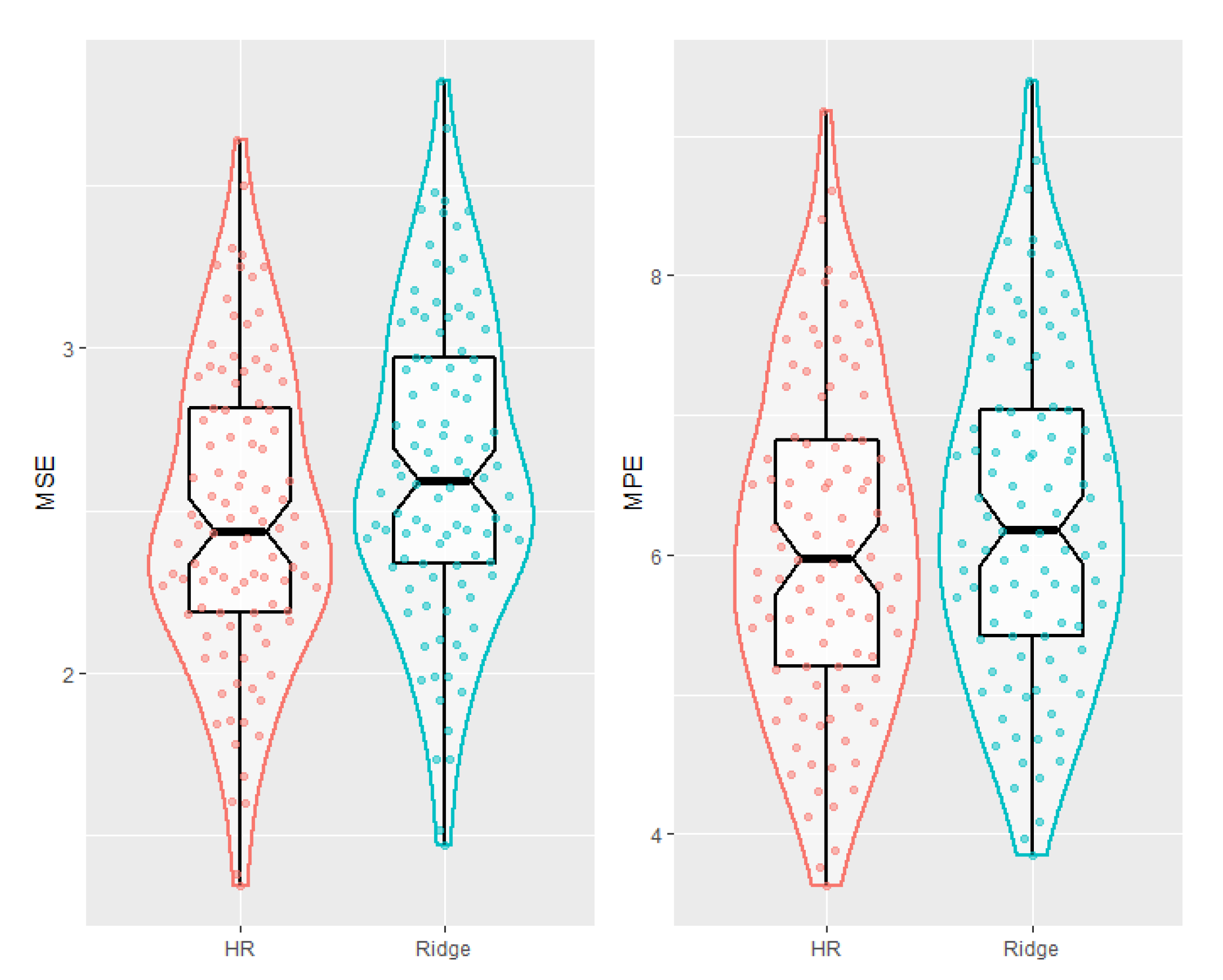
(1)

Using the GCV, the proposed estimator is shown to be consistently superior to the ridge estimator, relative to RMSE and RMPE criteria.

(2)

Similarly to the results of simulations, with growing p, the MSE of the proposed estimator increases compared to the ridge estimator. However, as p gets larger the mean prediction error becomes smaller, which shows the superiority for prediction purposes.

Further, Figure 2 depicts the MSE and MPE values for both HD and ridge estimators, for the case $p=1000$. It is obvious that the high-dimensional estimator performs better compared to the ridge. For the case $p=2000$, we obtained similar results.

Figure 2. Box-plot of the MSE and MPE values for $p=1000$ in the AML data.

5. Conclusions

In this note, we propose a high-dimensional two-parameter ridge estimator to the conventional ridge and Liu estimators. Its asymptotic properties have also been discussed. This estimator, via simulation and real-life experiments, is efficient in high dimensional problems and can potentially overcome multicollinearity. Additionally, the proposed high-dimensional ridge estimator yields superior performance in the small mean squared error sense.

References

- Hoerl, A.E.; Kennard, R.W. Ridge regression: Biased estimation for non-orthogonal problems. Technometrics 1970, 12, 55–67. [Google Scholar] [CrossRef]
- Tikhonov, A.N. Solution of incorrectly formulated problems and the regularization method. Sov. Math. Dokl. 1963, 4, 1035–1038. [Google Scholar]
- Saleh, A.K.M.E.; Arashi, M.; Kibria, B.M.G. Theory of Ridge Regression Estimation with Applications; John Wiley: Hoboken, NJ, USA, 2019. [Google Scholar]
- Wang, X.; Dunson, D.; Leng, C. No penalty no tears: Least squares in high-dimensional models. In Proceedings of the 33rd International Conference on Machine Learning, New York, NY, USA, 20–22 June 2016; pp. 1814–1822. [Google Scholar]
- Bühlmann, P. Statistical significance in high-dimensional linear models. Bernoulli 2013, 19, 1212–1242. [Google Scholar] [CrossRef] [Green Version]
- Shao, J.; Deng, X. Estimation in high-dimensional linear models with deterministic design matrices. Ann. Stat. 2012, 40, 812–831. [Google Scholar] [CrossRef] [Green Version]
- Dicker, L.H. Ridge regression and asymptotic minimum estimation over spheres of growing dimension. Bernoulli 2016, 22, 1–37. [Google Scholar] [CrossRef]
- Liu, K. A new class of biased estimate in linear regression. Commun. Stat. Theory Methods 1993, 22, 393–402. [Google Scholar]
- Ozkale, M.R.; Kaciranlar, S. The restricted and unrestricted two-parameter estimators. Commun. Stat. Theory Methods 2007, 36, 2707–2725. [Google Scholar] [CrossRef]
- Wang, X.; Leng, C. High dimensional ordinary least squares projection for screening variables. J. R. Stat. Soc. Ser. B 2015. [Google Scholar] [CrossRef] [Green Version]
- Luo, J. The discovery of mean square error consistency of ridge estimator. Stat. Probab. Lett. 2010, 80, 343–347. [Google Scholar] [CrossRef]
- Amini, M.; Roozbeh, M. Optimal partial ridge estimation in restricted semiparametric regression models. J. Multivar. Anal. 2015, 136, 26–40. [Google Scholar] [CrossRef]
- Akdeniz, F.; Roozbeh, M. Generalized difference-based weighted mixed almost unbiased ridge estimator in partially linear models. Stat. Pap. 2019, 60, 1717–1739. [Google Scholar] [CrossRef]
- McDonald, G.C.; Galarneau, D.I. A Monte Carlo of Some Ridge-Type Estimators. J. Am. Stat. Assoc. 1975, 70, 407–416. [Google Scholar] [CrossRef]
- Zhu, L.P.; Li, L.; Li, R.; Zhu, L.X. Model-free feature screening for ultrahigh dimensional data. J. Am. Stat. Assoc. 2011, 106, 1464–1475. [Google Scholar] [CrossRef] [PubMed] [Green Version]
- Metzeler, K.H.; Hummel, M.; Bloomfield, C.D.; Spiekermann, K.; Braess, J.; Sauerl, M.C.; Heinecke, A.; Radmacher, M.; Marcucci, G.; Whitman, S.P.; et al. An 86 Probe Set Gene Expression Signature Predicts Survival in Cytogenetically Normal Acute Myeloid Leukemia. Blood 2008, 112, 4193–4201. [Google Scholar] [CrossRef] [PubMed]
- Sill, M.; Hielscher, T.; Becker, N.; Zucknick, M. c060: Extended Inference for Lasso and Elastic-Net Regularized Cox and Generalized Linear Models; R Package Version 0.2-4; 2014. Available online: http://CRAN.R-project.org/package=c060 (accessed on 1 January 2021).
- Montgomery, D.C.; Peck, E.A.; Vining, G.G. Introduction to Linear Regression Analysis, 5th ed.; Wiley: Hoboken, NJ, USA, 2012. [Google Scholar]