1. Introduction
The impacts of climate change are manifesting through rising sea levels, reduced ice cover, extreme weather events, erratic weather patterns, and record-breaking temperatures across the globe. The Intergovernmental Panel on Climate Change (IPCC) forecasts a temperature rise of 1.4 to 5.5 Celsius degrees over the next century. The IPCC projects that a temperature increase of 1 to 3 degrees over 1990 levels will not only have differential impacts across regions, but it may also have varying impacts across different economic sectors. Agriculture, due to the strong dependence of crop yields on both weather and climate, is one of the most climate sensitive sectors and is the focus of the current study. This study examines how climate change models can be used in portfolio optimization of loans to the agricultural sector, and how climate change impacts credit risk.
The impact of climate change on the regional and global production of cereals including wheat, rice, maize (which we call corn in this study), and soybean is performed in [
1] which shows that a large increase in global temperature may cause a substantial decrease in crop production both globally and across many regions by 2080. This result is supported by [
2], which demonstrates the negative impact of rising temperatures on the global production of wheat, corn, and barley.
Climate change impacts food production both through temperature changes and precipitation changes. A study [
3] analyzed the impacts of future climate scenarios of 2 degrees warming and 20% precipitation decline on corn yield at nearly 200 Sub-Saharan Africa sites, using the CERES corn model. The study predicts an impact of between 11.4% and 14.4% yield loss due to temperature alone, with an associated, but smaller, negative yield impact due to the decreased precipitation.
The influence of these changes may be substantial to national economies. A Ricardian cross-sectional approach is used in [
4] to examine the relationship between changing weather patterns and farming in Cameroon. The analysis reveals that an increase in temperature or decrease in precipitation can seriously damage that nation’s economy, as 80% of the population is involved in farming, which represents 30% of the national GDP.
Rising temperatures may have a different impact on the yields of crops by crop type and over different regions. In some cases the impact may be positive, and in other cases negative. For example, a study of agricultural climate impacts in Asia [
5] projects continental rice production to decline by 3.8% over the next century with declines to be most marked in Thailand, Bangladesh, southern China and western India, but with partially countervailing production increases for Indonesia, Malaysia, Taiwan, and other parts of India and China.
However, changing practices can mitigate the impact of climate change to some degree. Global Climate Models are used in [
6] to predict a global crop yield reduction by the 2050s due to temperature and precipitation changes if planting and harvesting dates remain unchanged; however, in temperate regions, 7–18% of expected losses might be averted by adaptation in planting dates and cultivar choices.
Many other studies, notably [
7,
8,
9,
10] are devoted to the assessment of the impact of weather on agricultural productivity. Most of these studies are region specific, as climate impacts can be hard to generalize more broadly.
Agriculture and Credit Risk
The sale of crops is the main source of farm income, therefore driving the ability of farmers to repay agricultural loans. Banks must quantify climate related credit risk to agricultural portfolios in order to hedge risk and make adequate loan loss provisions. Expert management of these risks will allow banks to achieve higher risk-adjusted returns.
The New Basel Capital Accord (Basel II) emphasizes the development of portfolio credit risk models to ensure the creditworthiness of banks [
11]. According to Basel II, agricultural loans can be treated as retail exposures instead of corporate exposures depending upon the loan size. Many portfolio credit risk models [
12,
13,
14,
15] have been developed for corporate exposures, but these are not generally applicable to agricultural loans [
11]. The changing climate is making it imperative for banks to measure their credit risk in the agriculture sector and make decisions on their investments accordingly to mitigate the credit risk imposed by climate change.
The profitability of banks is highly affected by non-performing loans [
16]. Credit scoring models [
17,
18,
19] and portfolio credit risk models [
11,
20,
21] can be used to control the credit risk inherent to agricultural lending. However, these credit risk models typically fail to consider the impact of climate change on the creditworthiness of farms. A very few researchers have considered the impact of climate change on agricultural loan portfolios. The first default risk model and portfolio credit risk model, which incorporated agriculture-specific risk factors (commodity prices and climate risk), was introduced in 2014 [
22]. The model concludes that climate risk factors are more important than commodity price volatility and encouraged future studies to investigate the relationship between regional climate patterns and crop yields. Another study [
23] investigated the impact of weather conditions on the credit risk of small-scale rice farmers in Madagascar. A recent study examined the impact of climate change on corn and soybean yield for 1959 to 2013 in Ontario region [
24] and indicated that trends in temperature and precipitation during that period have not resulted in appreciable threats to crop yields in the region. The impact of climate change on the credit risk of a Greek bank has also been studied [
25] and findings support the fact that climate risk is considerable and should be considered in credit management process. However, credit risk models which assess the impact of climate change on the credit risk associated with agricultural lending portfolios are still in their infancy and more research is required to quantify the impact of climate change on bank farm loan portfolios.
The above studies show that the impact of changing climate across regions and crops may vary over time, implying that banks may also have to view their optimal loan issuance as a time varying decision.
In this paper, we have designed a framework to determine the optimal agricultural lending portfolio under different climate change scenarios to control the climate related credit risk. We consider five climate scenarios and propose a credit risk model to determine the optimal lending portfolio for any crop yield under these scenarios. For the numerical study, we have restricted the application to corn farming in Ontario. We use the corn yield, simulated in [
26] for 10 regions of Ontario under the considered climate change scenarios and then the optimal lending portfolios for these 10 regions are determined. This methodology can help banks decide their lending portfolio in a given geographical region under different climate change scenarios and will provide them with the information to control climate related credit risk by updating their agricultural lending portfolio. Climate change can have potential effects on corn yield through adverse weather conditions [
27] but in this paper, we consider the effects of increased temperature on corn yield as a measure of climate change, excluding other potential effects and interactions.
The remaining paper is organized as follows. In
Section 2, we consider the five climate scenarios from no warming at all (+0
C) to a warming of +4
C over the next 49 years and discuss the crop yields simulated in [
26] for 10 regions of Ontario under considered climate change scenarios. A model to manage the credit risk is introduced in
Section 3 using the crop yield simulations discussed in
Section 2. The model is implemented for the corn yield in Ontario in
Section 4 and the obtained results are discussed in
Section 5. Finally, conclusions are made in
Section 6.
2. Climate Change Scenarios and Yield Simulations
We chose climate change scenarios between +0
C and +4
C by taking inspiration from a recent Climate Change for Ontario report [
28]. The climate change scenarios and the resulting simulated yield paths at the 2068 horizon for corn yield are based on the work, presented in [
26]. We consider 10 regions in Ontario, which are representative of the corn growing regions in the province: Brockville, Cornwall, Fergus, Kapuskasing, Kingsville, North Bay, Ottawa, Toronto, Trenton, and Woodstock. For each region, we consider five climate change scenarios at the 2068 horizon. Those scenarios represent situations ranging from no warming at all, which constitutes an hypothetical disappearance of the historical realized trend of +2
C over the past 49 years, to +4
C, representing an acceleration of climate change. Authors [
26] considered 1500 climate paths, presenting evidence that this number is sufficient to achieve stability in the distribution of the simulated corn yields for each year of the simulation between 2020 and 2068. The 1500 climate paths are obtained through a block bootstrap method on historical climate data, temperature, and rainfall, provided by the Global Historical Climatology Network Daily (GHCND) database of the National Oceanic and Atmospheric Administration (NOAA). The dates for the start and the end of the corn growing season are derived from the work [
29] by using a set of rainfall dependent rules detailed in [
26]. The simulated corn yield paths are obtained from the climate change paths by using the Corn Heat Units (CHU) formula detailed in [
30] and adopting a linear relationship between corn yield and CHU. The CHU is only dependent on daily minimum and maximum temperatures. The simulated corn yield paths created in [
26] are used in the calculations of the present paper. For a given scenario, the 1500 corn yield paths for each city are obtained by using simulated climate variable paths (minimum temperature, maximum temperature, and rainfall) computed from historical climate data using a block-bootstrap technique.
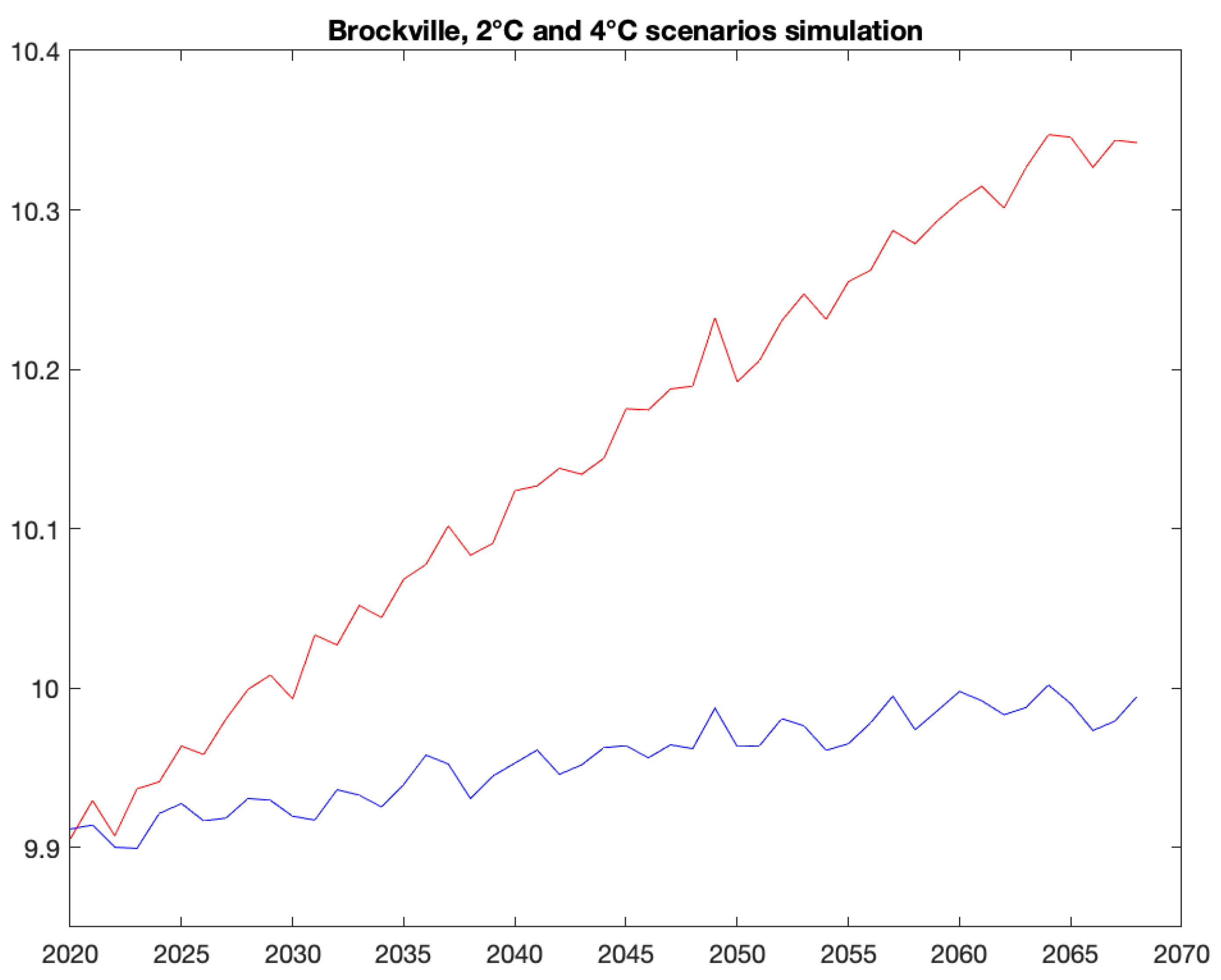
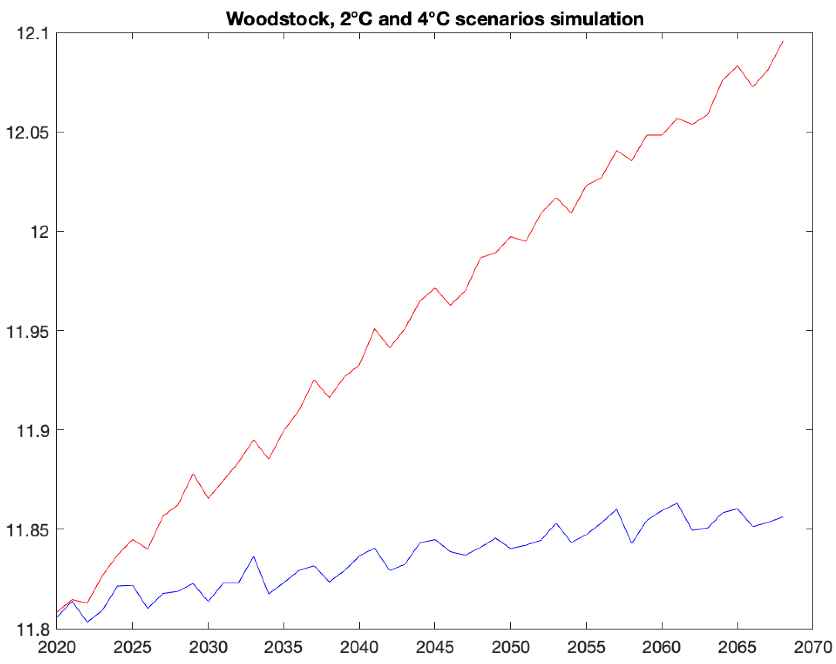
Figure 1 and
Figure 2 depict the simulated corn yield, averaged over the 1500 paths, for Brockville and Woodstock under the +2
C (blue) and +4
C scenarios.
In the next section we discuss how these changed corn yields impact the performance of agricultural loan portfolios.
3. Credit Risk Management
As the changing climate may affect the crop yield in different regions differently, here we consider n different regions. Our model provides us with the optimal loan portfolio under a given climate change scenario, which would help the banks to decide on their budget allocation to n regions in order to minimize their credit risk for a given minimum acceptable level of return. For banks, the return on loans is the rate of interest in any region. The rate of interest typically varies depending on loan tenor and may vary depending upon tenor. So, we categorize the loans of jth region into m categories on the basis of their tenor. The represents the total amount that jth region is asking for loans of tenor i years, for all and . Banks often organize their loan portfolios to ensure that they have a balance of tenors. Insurance companies, which may also invest in creditworthy loans, are often guided to various loan portfolios by asset liability matching considerations.
The regions can request loans for different tenors, but it is not always possible for banks to provide the entire amount requested in a given region and tenor bucket due to budget or risk constraints. Suppose the total amount
is requested by region
j for loans of tenor
i. Then a vector of decision variables
x is chosen
where
represents the proportion of
allocated to
jth region for loans of length
i years.
The
represents the amount allocated to region
j for loans of
i years. So, the vector
represents the loan portfolio for
m types of loans in
n regions. Adding up the allocations for different tenor loans to the
jth region provide us with the total allocation
to the
jth region. The allocation to each region is assumed to be non-negative and may have some specific lower
and upper bound
.
where
B represents the total budget.
These regional investments should satisfy the following budget constraint
We have
m types of loans in each region and the entire investment amount should not be allocated to any specific tenor loans, so we assume the lower bound
and upper bound
for the allocation to loans of tenor
i years, satisfy the following constraints
Let
S be the feasible set of loan proportions
, consisting of constraints (
1)–(
4). Thus,
where
.
3.1. Return on Agricultural Loans
We assume the farmers repay the loans at maturity, so a compound rate of interest is used to estimate the return on loans. Assume the parameter
represents the compound rate of interest for the loans of tenor
i years in all regions. The rate of interest on different tenor loans across all regions is the only return of banks on agricultural loans. So, the total return on agricultural loans
across all regions is calculated as
3.2. Credit Risk in Agricultural Loans
Agricultural Credit risk is the loss arising from the inability of farmers to fully repay their loans. As such, this is strongly determined by farm income, for which an important factor is crop yield. The crop productivity may be influenced by regional climate conditions, so we use a simulated yearly crop yield distribution
(consisting of 1500 crop yield pathways discussed in
Section 2) for the
jth region to estimate the crop yield in year
t under a given climate change scenario
C. The credit risk across all the regions is assessed using their respective crop yield distributions.
The proportion of loan size that farmers may default is considered as the credit risk. The farmers may default on payment whenever their loan size is higher than their farm income. For example, if a farmer takes a loan of
for two years at a
annual rate of interest and the two-year farm income is
, then the default will be
. To estimate the highest expected credit risk, we use the risk metric Conditional value at risk (CVaR) at level
, which provides us the average of
worst credit risks (losses). We use the CVaR risk metric to quantify the credit losses as it is a coherent (a risk measure is coherent if it is translation invariance, subadditive, positively homogeneous, and monotonic) [
31]. risk measure and can be easily incorporated in optimization, and specifically it is convex and sub-additive so it supports loan portfolio diversification.
To estimate the credit risk CVaR, first we construct credit loss distributions
for different tenor loans in all the regions by using the simulated crop yield
of the respective region. The credit loss distribution for
i year loans to farms in region
j can be calculated as
where
- (a)
represents the total repayable loan amount for the loans of tenor i years in region j;
- (b)
represents the total land area (in hectares) used by farmers to grow the considered crop in region j who are requesting loans for tenor of i years;
- (c)
Crop can be sold for per ton;
- (d)
represents the sum of crop yields for next i years and is the simulated crop yield (tons/hectare) for year t under climate change scenario.
Consider a random variable
for the credit risk that depends on the random credit losses
and the proportion of the loans vector
across all the regions. The risk measure CVaR
, for a given a parameter
, can be calculated as [
32]
where
,
represents the expected value and
l represents value at risk (VaR) that is obtained as a by-product while minimizing CVaR [
32]. The parameter
q represents the total simulated crop yield pathways and
is the probability of occurrence of
kth pathway. For any given
kth pathway, if Equation (
10) yields a value greater than
l then it contributes to CVaR and represents the total default amount across the regions associated with portfolio
. We have 1500 simulated crop yield pathways so
and
for all
k (each yield pathway is assumed equiprobable).
3.3. Model to Minimize Credit Risk
The model to minimize CVaR
for some given acceptable minimum level of returns
R is formulated as
Considering
q auxiliary variables
, the model (
11) can be transformed into the following model
The resulting problem (
12) is linear in
and
and can be solved by using the simplex method.
Remark 1. The lending portfolio can be calculated under any climate change scenario with a warming of C () by using the crop yield distributions of respective climate change scenarios in model (12). 4. Application to Corn Yield in Ontario
In this section, the optimal lending portfolio is obtained to make loans backed by corn farm income in the 10 corn producing regions of Ontario. We use the simulated corn yield, computed at 10 regions, over the next 49 years under
C climate change scenarios,
[
26]. For a given scenario, we have 1500 (deemed equiprobable) crop yield paths for each region and for each year between 2020 to 2068. Thus, we have a discrete uniform crop yield distribution
for each region
j and each year
, under a given climate change scenario
C.
We consider banks making loans for the tenor of
i years
at their respective rate of interest, provided in
Table 1. The rate of interest for chosen loan tenors are obtained from the Scotiabank Canada website (
https://www.scotiabank.com/ca/en/personal/rates-prices/mortgages-rates.html) accessed on 15, July 2020. The obtained fixed annual rate of interest is used to calculate the compound rate of interest
for the entire loan tenor. We assume farmers repay the loans (principal amount and rate of interest) at maturity.
The method can be used to determine the optimal lending portfolio for future years as well if the required data are available. Our focus is to determine the optimal lending portfolio for a recent year 2020 () under C climate change scenarios for . Due to the dearth of data, we need to make the following realistic assumptions:
The lower limit
and upper limit
for budget allocation to regions, defined in Equation (
2), help to diversify the lending portfolio across the regions. The lower limit
is assumed to be
of the budget for
and the upper limit
is calculated by using the percentage land area of
jth region used for harvesting corn yield in 2019, described in
Appendix A. The data for land area have been obtained from OMAFRA (
http://www.omafra.gov.on.ca/english/stats/crops/(accessed on 5 May 2021));
The lower limit
and upper limit
for budget allocations to different type of loans, defined in Equation (
4), help to diversify the portfolio across different tenor loans. The lower limit
is assumed to be
of the budget for
. The upper limit
is assumed to be
of the budget for
(The upper limit is assumed to be
higher than
(equal distribution) as if all the
budget is going to be used then allocations to different tenor loans do not hit their upper bounds.);
We assume the land area , used by farmers in jth region who seek loans for tenor i years, is equal for all and . As we have seven different tenor loans, we assume banks have to lend out each type of loan per unit land area in each region. We have estimated the crop yield per unit land area in each region, so we assume the loan size on unit land area as well;
The minimum acceptable return
R is assumed to be 30% of the total budget. The lenders can define any achievable return threshold. We want to invest the entire budget so we consider the budget constraint (
3) as an equality constraint in our numerical study;
We assume the loan size of
i year loans is proportional to the farmers’ incomes for
i years. We estimate the farmers’ income in two ways, using their historical crop yield and the simulated crop yield. The size of
i year loans for the
jth region is calculated as
where
is the historical corn yield of
jth region in year 2019 (transformed in metric tons/hectare), retrieved from OMAFRA (
http://www.omafra.gov.on.ca/english/stats/crops/ accessed on 5 May 2021). Corn can be sold for
CAN per ton [
26]. The simulated loan size is estimated using the expected simulated crop yield
of year 2020 (first year) under +0
C scenario.
In
Section 4.1 and
Section 4.2, we determine the optimal lending portfolio under five climate change scenarios using the historical and simulated loan sizes.
4.1. Optimal Lending Portfolio with Historical Loan Size
We obtain the optimal lending portfolio for 10 regions under different climate change scenarios
C (
), using the method described in
Section 3 using a
confidence level
.
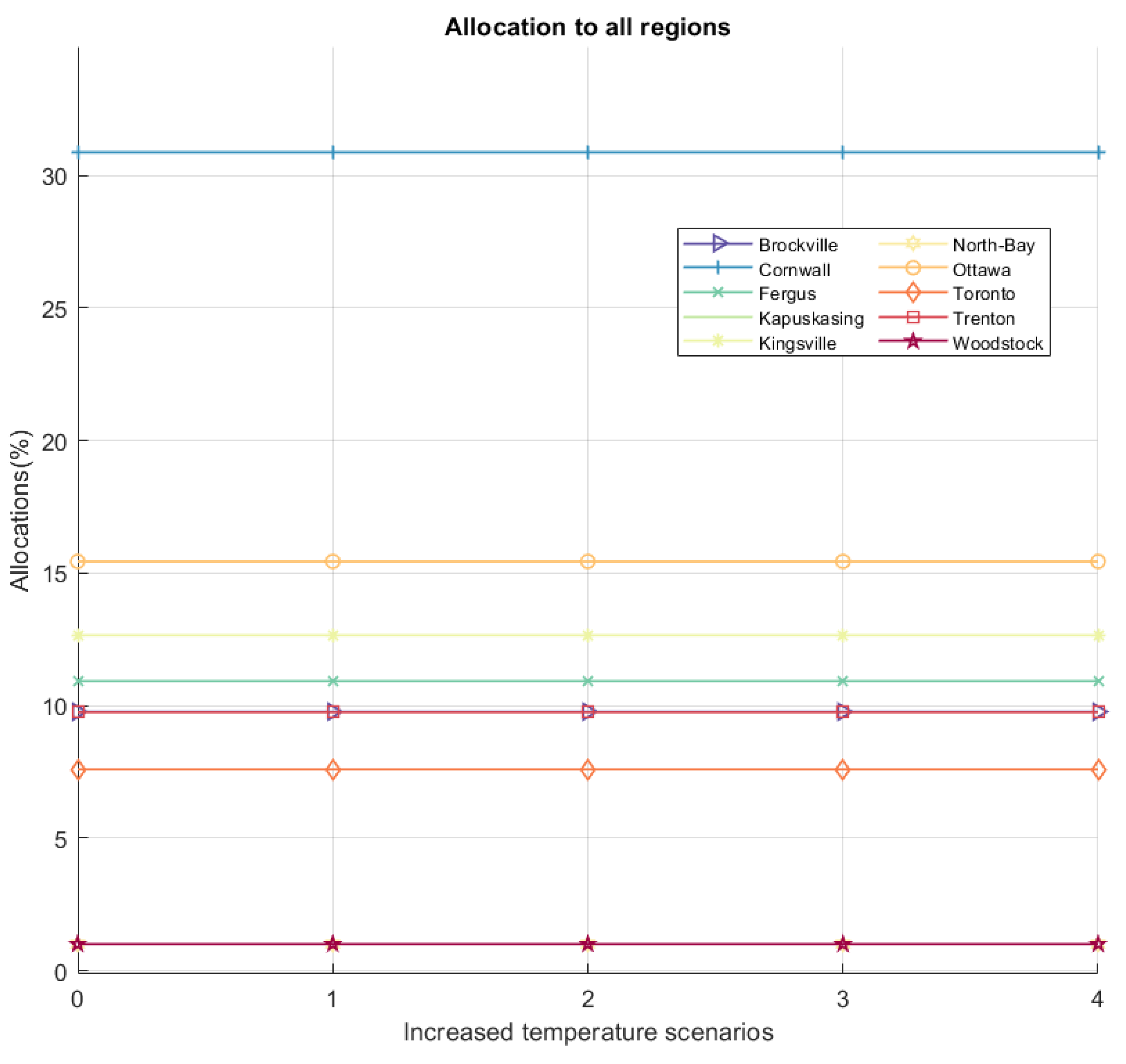
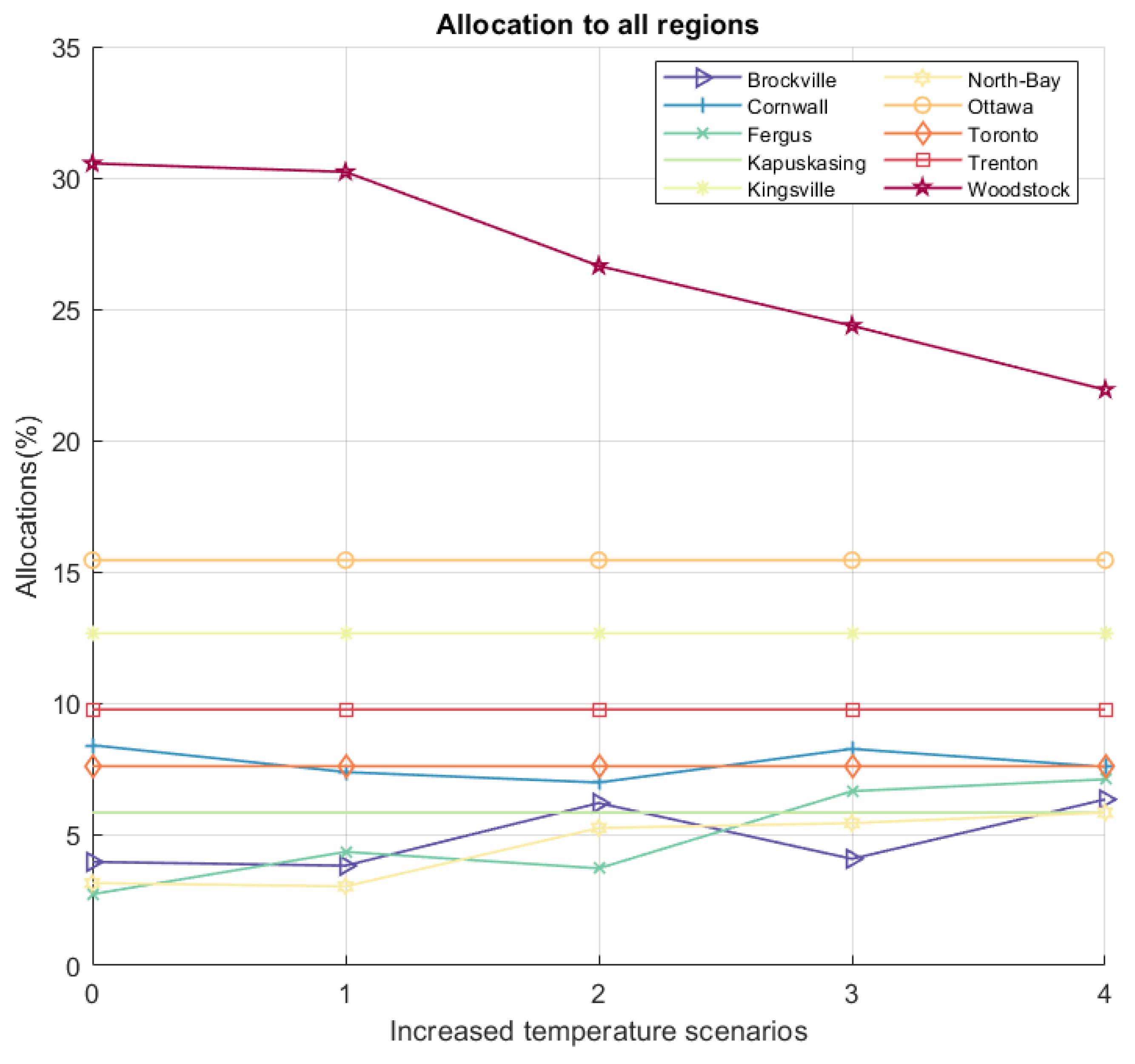
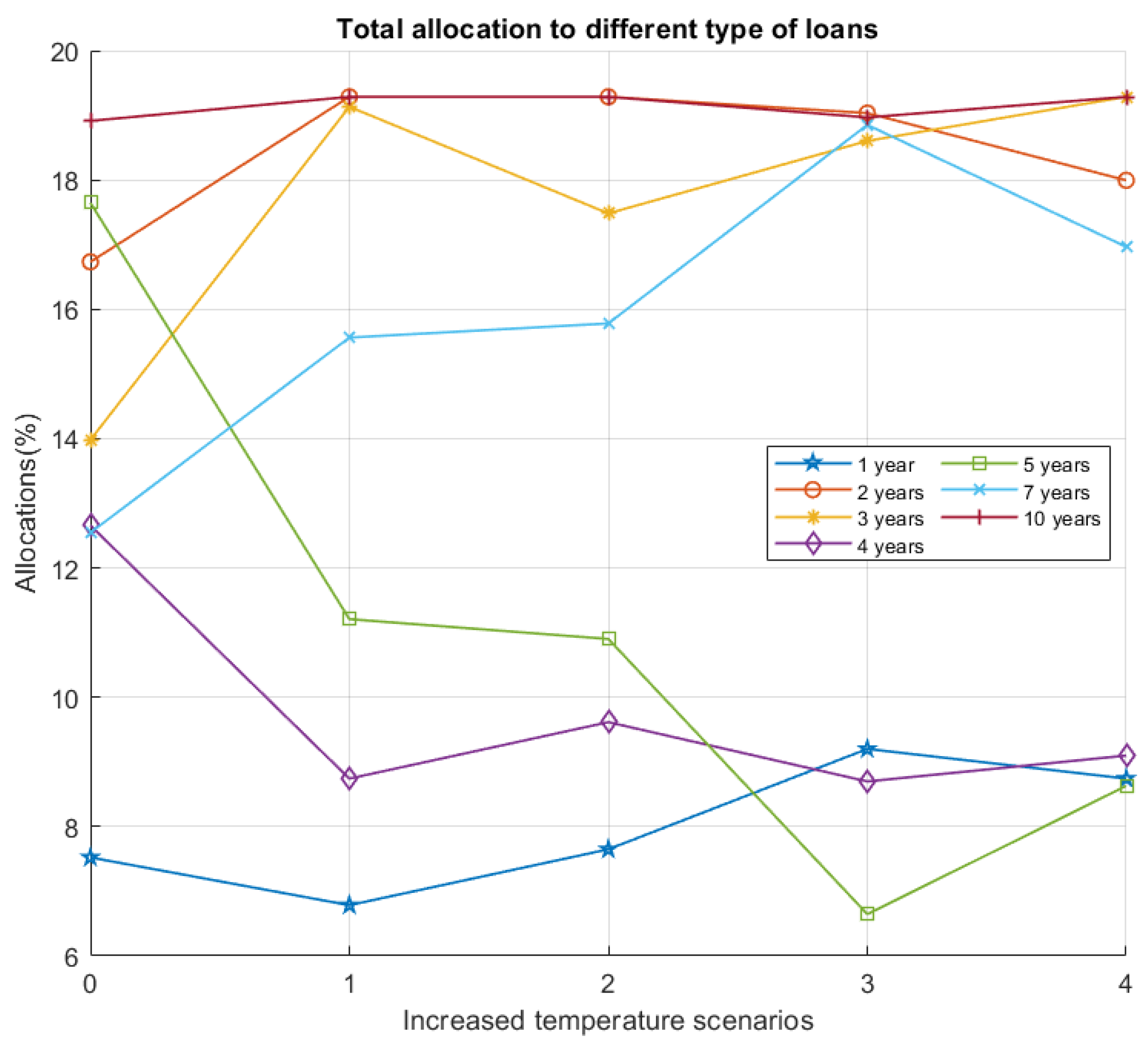
Figure 3 demonstrates the optimal allocation (percentage of budget) to each region under different climate change scenarios and
Figure 4 shows the optimal allocation to each tenor loan under different climate change scenarios.
Figure 4 shows that the allocations to different tenor loans are changing under different climate change scenarios.
The lending portfolios, across regions, under different climate changes depicted in
Figure 3 remain the same, as we consider only loans with maturities up to 10 years, which is not a very long period to calibrate the impact of climate change. However, the allocations to loans of different tenor change a great deal as we move from the +0
C to +4
C degree scenarios presented in
Figure 4.
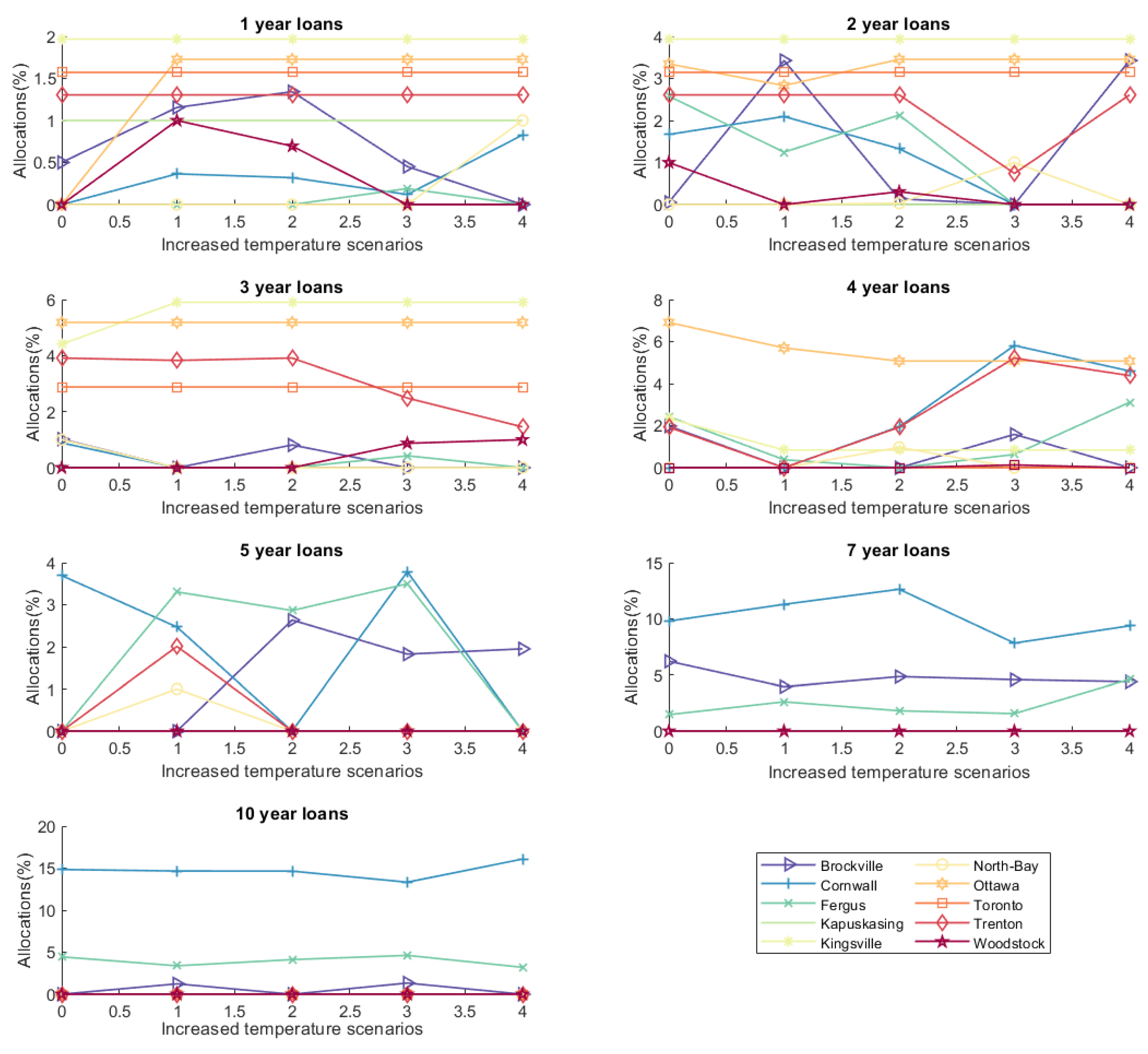
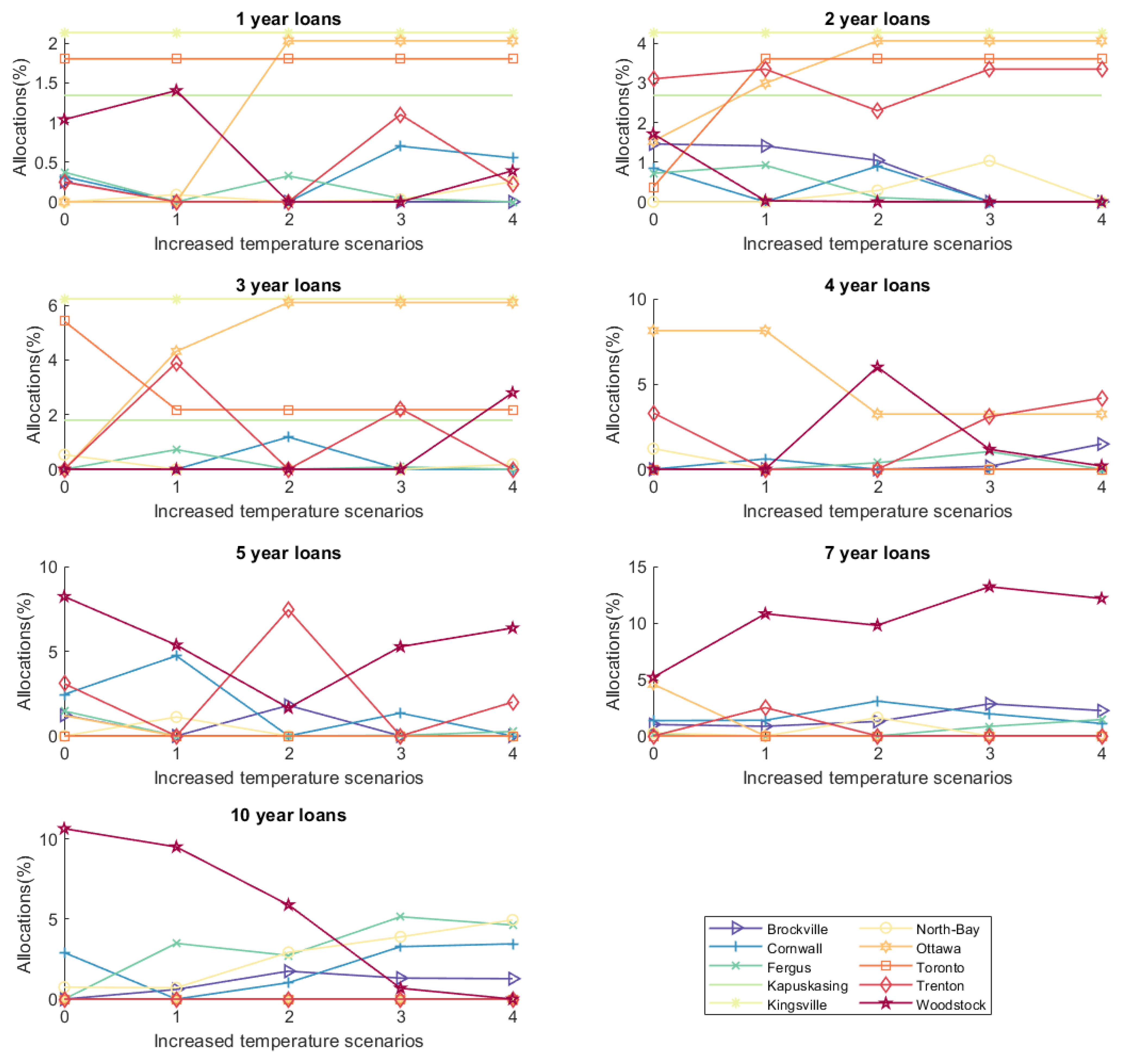
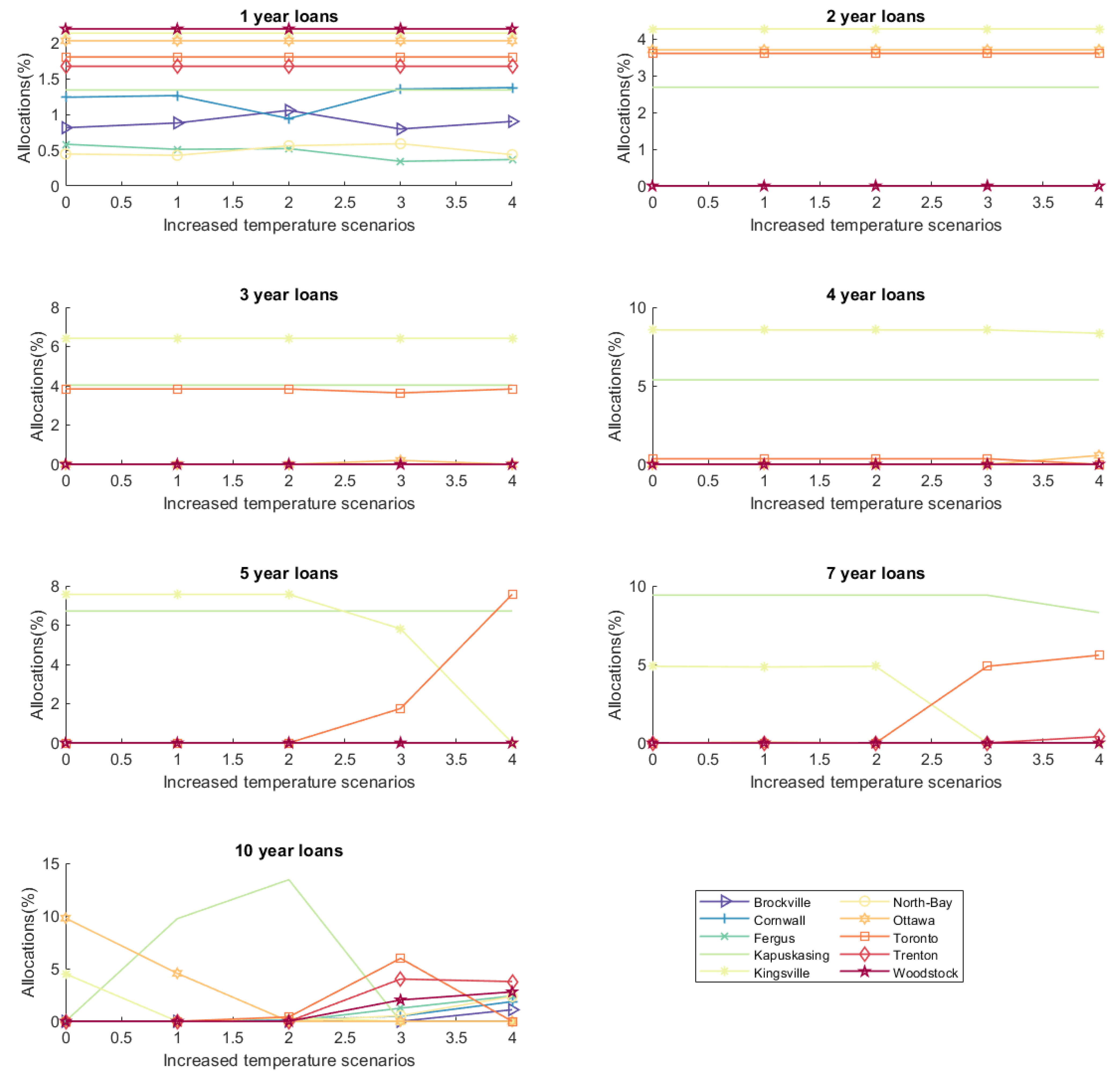
It is expected that if rising temperatures are beneficial for crop yield in a region, then its longer tenor loans should be more favorable and if rising temperatures have an adverse affect on crop yield, then allocation to short tenor loans should be less risky. To gain insight into the variations in allocations to different tenor loans we need to look into the allocations to different tenor loans in all the regions explicitly. For that, we plot the optimal allocation to each tenor loan in each region under different climate change scenarios, as exhibited in
Figure 5.
To check the consistency of the lending portfolio (presented in
Figure 5) with the crop yield simulations, we categorize the regions according to their expected crop yield in the 49 years from 2020 to 2068 [
26] as follows
More favorable: Rising temperatures would be most favourable to the regions around Brockville, Cornwall, Fergus, North Bay, and Woodstock as their crop yield is expected to increase with rising temperature. The benefit to crop yield in the Woodstock region is lower than in other regions.
Less favorable: The regions around Kapuskasing, Toronto, and Trenton are expected to experience a small gain in their crop yield due to rising temperature. The gain in crop yield is comparatively higher in Trenton.
Not favorable: In contrast, the crop yield around Kingsville and Ottawa may experience declining crop yields if temperatures rise.
The impact of climate change on allocation to different tenor loans may vary as the impact of climate change is more apparent on longer periods than short. So, the allocation to 10 years loans will be more influenced by climate change because of its longer tenor. The impact of climate change may decrease as the length of loans decrease. Our crop yield variation is estimated for the period of 49 years and loans are of length up to 10 years, so the allocations are not expected to track crop yield variations exactly, but the allocations are still consistent with expected crop yield, as described below
Allocation to 10 year loans to ‘More favorable’ regions increases as the temperature rises from C to C. We have restrictions on allocations to different tenor loans so it is not possible to make allocations to longer tenor loans in all the ‘More favorable’ regions. So, the allocations to other loans increase in North Bay and Woodstock rather than longer tenor loans as the other loans are also profitable;
The ‘Less favorable’ regions are expected to get very little benefit from rising temperatures so they have no allocations to longer tenor loans. Kapuskasing and Toronto are expected to get the least gain in crop yield. It is almost negligible, so its allocations remain the same under all the scenarios. Trenton is expected to benefit more than Kapuskasing and Toronto so its allocation to average tenor loans (2 years loans, 4 years loans) increase as the temperature rises;
On the other hand, allocations to even average tenor loans (4 years loans) to the ‘Not favorable’ regions decrease and allocation to short tenor loans (Kingsville—3 years loans, Ottawa—1 year and 2 years loans) increases as the temperature rises, and allocations to other short tenor loans remain the same (Kingsville—1 year and 2 years loans, Ottawa—3 years loans).
These allocations are also influenced by the upper limit for allocations to all regions. The allocations are influenced by these restrictions and climate change as well, so to assess the impact of only climate change we relax some restrictions in the following subsection.
Quantify the Impact of Climate Change on Lending Portfolio
Our focus in this subsection is to investigate the impact of climate change on credit risk and see how the lending portfolio is changing under different climate change scenarios. Therefore, to capture the impact of climate change only, we relax the following restrictions on constraints that can influence the portfolio:
The lower bound on allocations to regions and lower bound on allocations to different tenor loans are assumed to be 0;
The upper bound on allocations to regions are set to infinity;
The minimum acceptable return limit may have an impact on allocations, so it is assumed to be 0.
We consider the following different tenor loans to quantify the impact of climate change on allocations:
- (i)
Allocations to one type of loans: Assume we have only one year loans, so we invest the entire budget amount in one year loans using upper bounds on different tenor loans
(of budget) and
. The allocation to one year loans is affected by climate change in Brockville and Fergus, presented in
Figure 6. Similarly, if we assume only two year loans (
and all other values of
, then only the allocations to Brockville and Fergus are impacted by climate change, as depicted in
Figure 6, and the allocations to the remaining regions remain the same under different climate change scenarios.
- (ii)
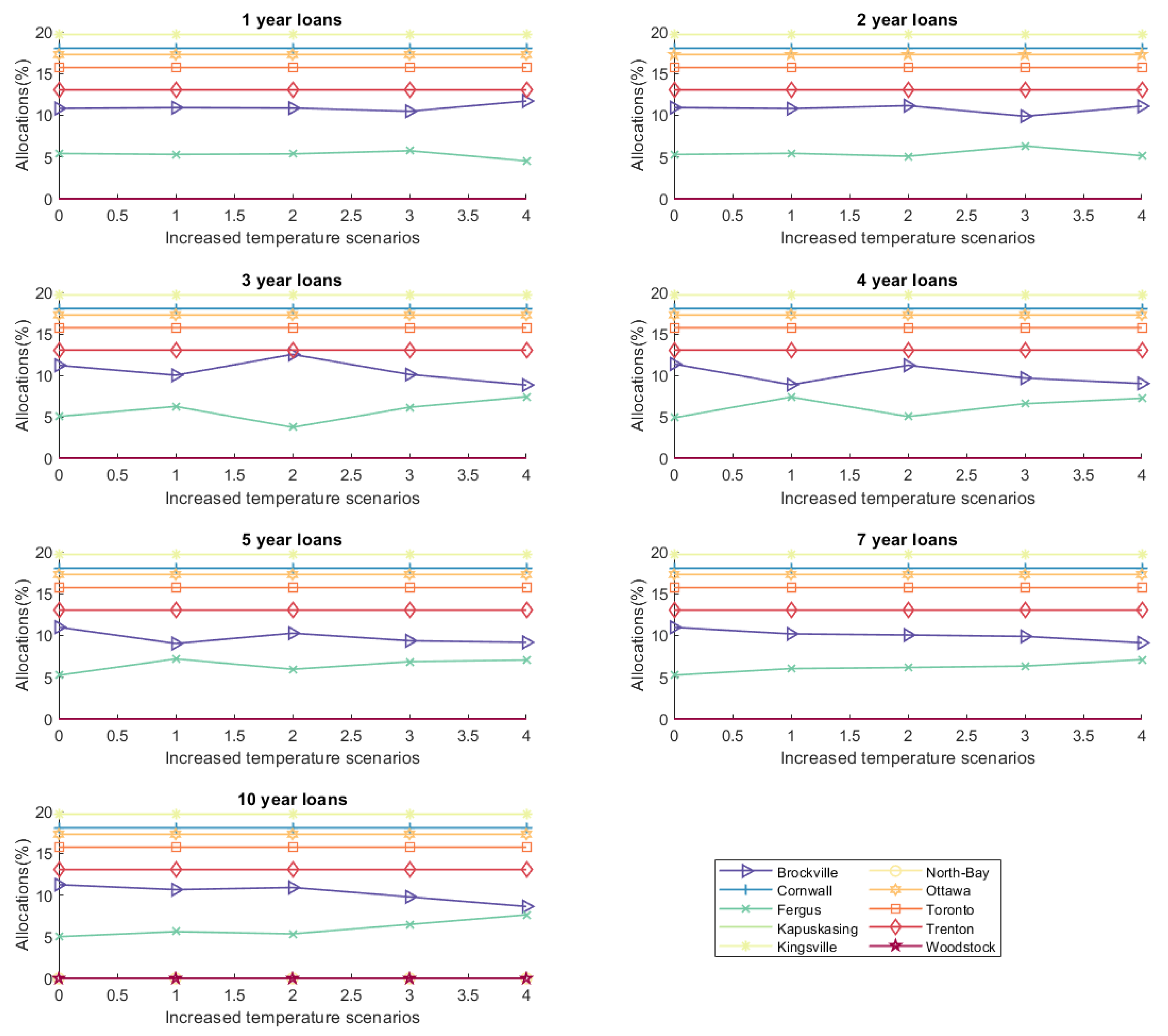
Equally balanced portfolio: We consider all the seven type of loans in all the regions and equally distribute the budget amount among these loans using upper bounds on different tenor loans
. The impact of different climate change scenarios on allocations is presented in
Figure 7.
The change in allocations appears to occur because of climate change. We see little change in allocations as we use historical loan size. Historical loan size need not to be close to the simulated farm income (depends upon simulated crop yield) and whenever the difference between simulated farm income and loan size is larger than the change in crop yield (farm income) caused by climate change, allocations may not change. So, to capture the impact of climate change more appropriately we consider the simulated loan size in the following section so that the loan size remains closer to the simulated farm income.
4.2. Optimal Lending Portfolio with Simulated Loan Size
In this section, we obtain the optimal lending portfolio for 10 regions under different climate change scenarios using simulated loan size and using a
confidence level.
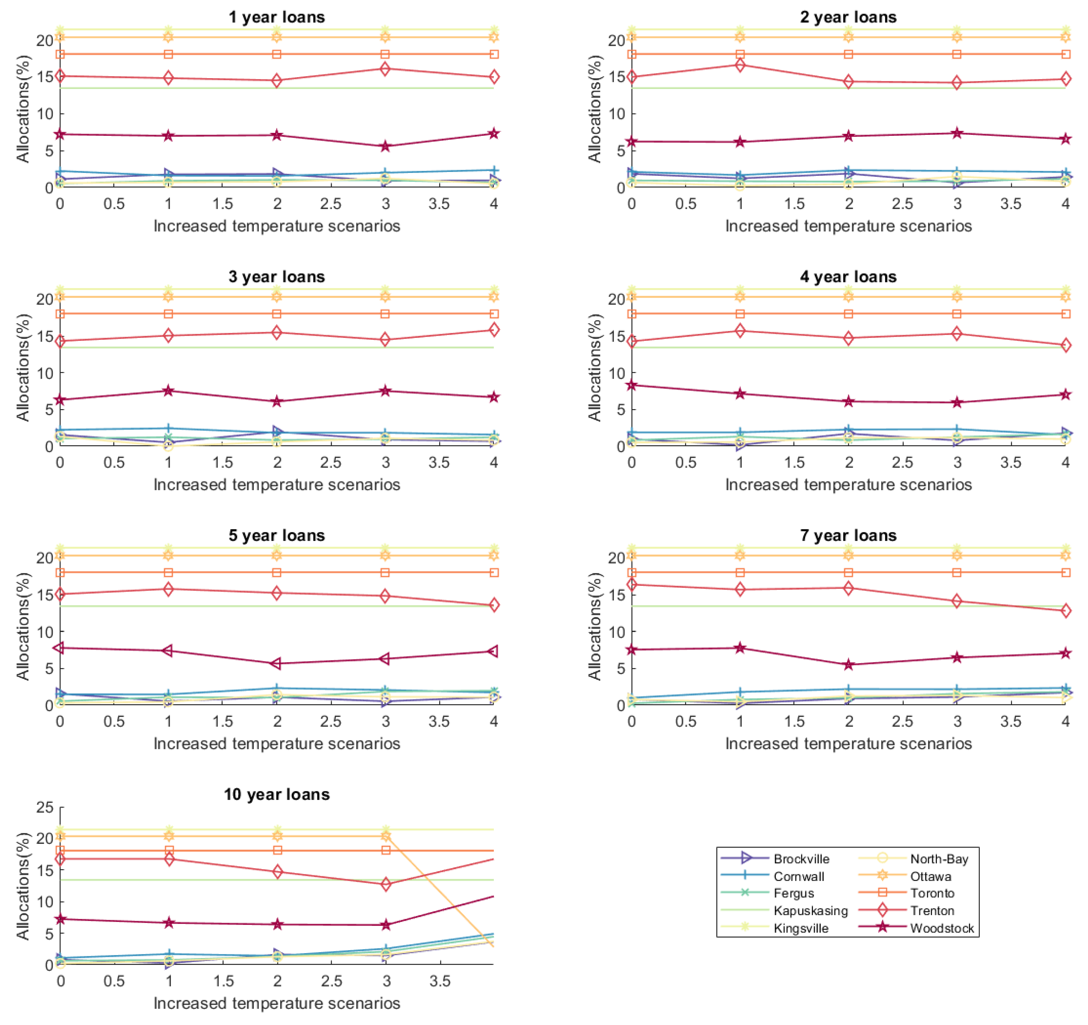
Figure 8 and
Figure 9 display the allocations to all regions and all tenor loans, respectively, under different climate change scenarios. The allocations to Brockville, Cornwall, Fergus, and North Bay are increasing and the allocation to Woodstock is decreasing as the temperature rises, as demonstrated in
Figure 8. While Woodstock may expect increased crop yields with risking temperatures, its allocations nonetheless decrease. This is because its loan size is the highest amongst all regions, reducing diversification risk reductions.
The allocations to loans of different tenor change a lot as we move from +0
C to +4
C, as shown in
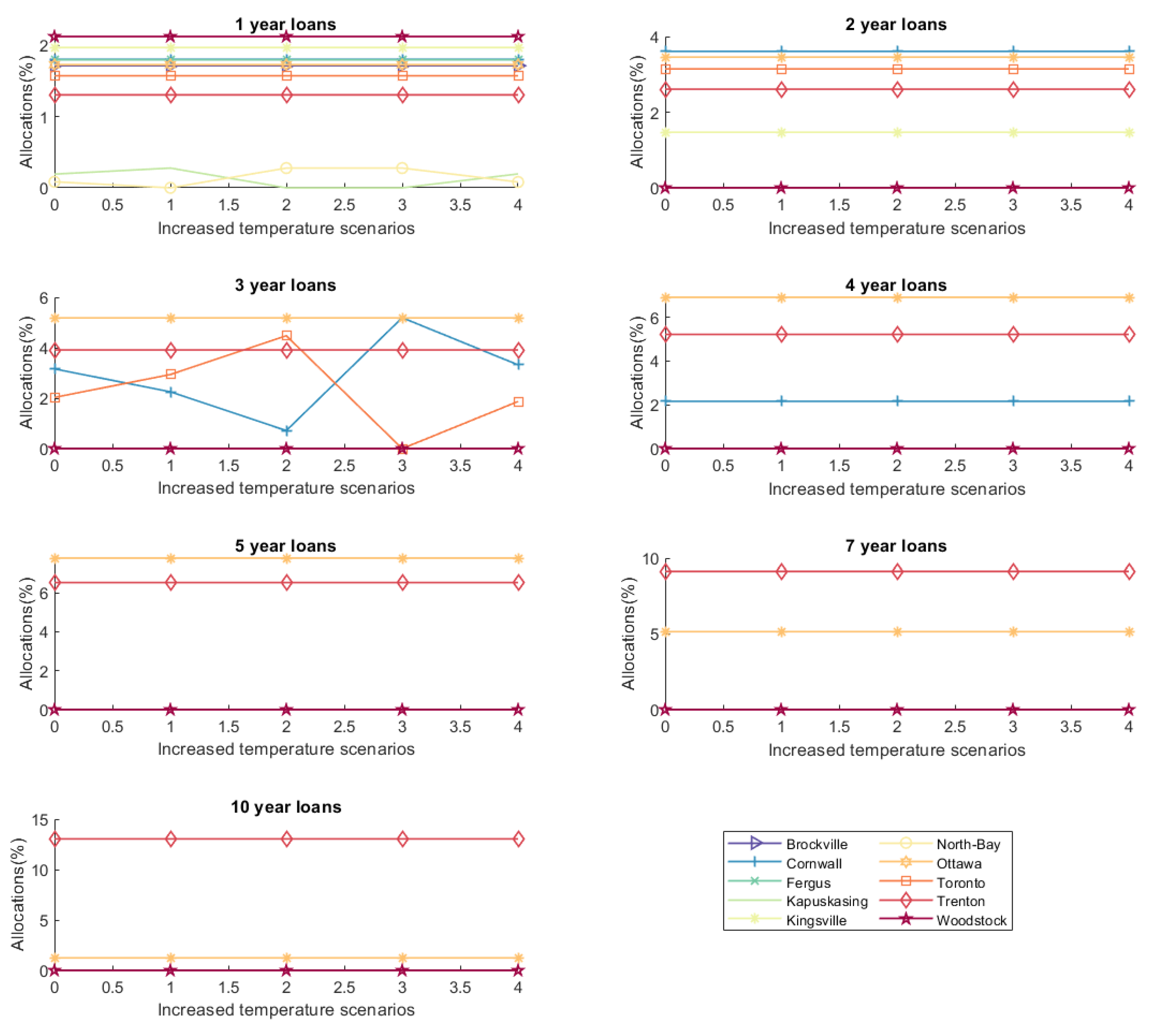
Figure 9. To better appreciate these variations in allocations to different tenor loans we examine the allocations to different tenor loans in each region explicitly in
Figure 10. The consistency of variation in crop yield with variation in allocations can be understood as follows:
Allocation of 10 year loans to ‘more favorable’ regions increases as the temperature rises from +0 C to +4 C. Due to restrictions on allocations, it is not possible to make allocations to longer tenor loans in all the ‘more favorable’ regions. So, the allocations of 7 years loans increase in Woodstock rather than 10 years loans;
The ‘less favorable’ regions are expected to get very little benefit from rising temperatures so they have no allocations to longer tenor loans. Kapuskasing is expected to get only a negligible increase in crop yield so its allocations remain the same under all the scenarios. Toronto is favorable for 1 and 2 year loans and the allocation of 3 year loans decreases as the temperature rises. Trenton is expected to get more benefit than Kapuskasing and Toronto, so it has some allocations to 1 to 5 years loans with few fluctuations as the temperature rises;
Allocations of average tenor 4 year loans to the unfavorable Ottawa region decrease but allocations of short tenor loans (1 to 3 years) increase with the temperature rise. The allocation to 1 year loans to Kingsville increases as the temperature rises, and allocations to 2 years loans remainsvery small with little fluctuations as the temperature rises.
These allocations may also be influenced by the restrictions on allocations and return threshold level. So, to assess the impact of only climate change, we relax some restrictions that may influence the allocations in the following subsection.
Quantify the Impact of Climate Change on Lending Portfolio
To assess the impact of climate change only, we relax restrictions as in Subsection and consider the following tenor loans to quantify the impact of climate change alone on allocations:
- (i)
Allocations to one type of loans: We assume only one type of loans (one year loans or two years loans or so on) and invest the entire budget one type of loan. The allocations to the regions are depicted in
Figure 11;
- (ii)
Equally balanced portfolio: We again consider the equally balanced portfolio as described in Section. The impact of different climate change scenarios on allocations is presented in
Figure 12.
It can be observed from
Figure 11 to
Figure 12 that the impact of climate change on 1 to 4 year loans is comparatively less than 5, 7, and 10 year loans. If the temperatures rise then banks should increase their investment in Brockville, Cornwall, Fergus, North Bay, and Woodstock for longer tenor loans.
5. Results and Discussion
In this section, we use the methodology developed until this point to quantify the impact of climate changes on the credit risk of agricultural loans made to Ontario corn farmers.
Our work assumes a bank operating a notional $100,000 Canadian dollar loan portfolio. We calculate the credit risk at (aggregated multi-year) return threshold levels of 30%, 20%, and 15% across the following two cases:
Considering climate change: Here, credit risk is assessed assuming the bank lends across the 10 climate regions using the climate impact modeling presented here (climate warming scenarios; crop yield impact). As such, the bank opts to lend according to the optimal portfolios obtained in
Section 4.1 (for historical loan sizes) and
Section 4.2 (for simulated loan sizes), respectively. Each of these portfolios are crafted for each of the five climate change scenarios for 0, 1, 2, 3, and 4 Celsius degrees warming. The results of this analysis are presented in the left-hand columns of
Table 2 (historical) and
Table 3 (simulated) loan sizes;
Neglecting climate change: Some banks may prefer not to explicitly incorporate the impact of climate change in their portfolio modeling, because of uncertainty around exactly how climate change might manifest, or to minimize model risk. To capture this approach, we determine the optimal lending portfolio across the 10 regions using historical corn yield data from 2019, obtained from OMAFRA
http://www.omafra.gov.on.ca/english/stats/crops/ accessed on 5 May 2021, and assume that these yield data will remain invariant. Despite their assumptions, in our analysis of their portfolio, we nonetheless assume that temperatures will change, again using the same five ttemperature growth scenarios as in the “Considering climate change” section above. The results of this analysis are presented in the right-hand columns of
Table 2 (historical) and
Table 3 (simulated) loan sizes.
The results contained in
Table 2 and
Table 3 demonstrate the increase in risk associated with ignoring climate change. This risk decreases “down the table” as target returns reduce, as is common in finance. This increased risk makes sense—models that do not account for changing situations are less well adapted to their world than those that do account. It is interesting though that the increase in the simulated risk (
Table 3) scenario is relatively modest, but in the historical risk (
Table 2) scenario, much more so.
In all cases the risk reduces as the temperature warms: this is because, for heat loving corn in a region where drought is not a big issue, temperature change is actually a yield increasing fact.
The results also demonstrate that model risk matters if we use the historical loan size and it does not matter much if the simulated loan size is used. The historical loan size is smaller than the simulated loan size, so we get the benefit of smaller loan size and climate change both by considering ‘Climate change’ rather than ‘Neglecting climate change’. On the other hand, the simulated loan size is higher (proportional to simulated crop yield income) which makes it more risky for both cases ‘Climate change’ and ‘Neglecting climate change’. Generally, we expect the loan size to be similar to the historical loan size than the simulated loan size.
6. Conclusions
This paper explores the use of a biologically-inspired method for connecting climate change scenarios to corn yield scenarios to simulate farm income, and hence the chance of loan losses to agricultural loan providers investing across a portfolio of Ontario, Canada, corn farming risks. The results show that, depending on the modeling approach chosen, the use of climate change models can provide significant (historical approach) or more modest (simulated approach) risk reductions.
It should be noted that Ontario rarely suffers from drought, and so the impact being quantified here is on a warming climate alone. The corn plant is fairly heat loving, so this impact is generally positive. The success of this case study suggests that extension of this idea to a less heat loving crop (e.g., wheat) in a region where climate change impacts may also lead to less rainfall (e.g., Western North America) might be very fruitful.
This study is focused on portfolios of loans made to corn farmers in the Ontario region. The results of this study cannot immediately be generalized to other regions with different characteristics. There is, however, scope to generalize the methodology presented here to other crops, or other regions, by introducing appropriate variables according to the specific crop response attributes and regional climactic conditions. In addition, this case study incorporates the impact of climate change only via differing temperature increase scenarios. Other possible climate change impacts, such as severe weather patterns, are not considered here, providing more avenues for future work.
Author Contributions
J.K.B.: optimization models, implementation, data analysis, writing; A.K.: climate models, data analysis, writing; W.J.B.: statistical and climate models, graphics, proofreading; M.D.: problem conception, finance research, writing; W.H.: optimization models, proofreading. All authors have read and agreed to the published version of the manuscript.
Funding
This research was funded by Natural Sciences and Engineering Research Council of Canada (NSERC), funding reference numbers 2018-03865 and 2020-06667, and Bank of Nova Scotia.
Institutional Review Board Statement
Not applicable.
Informed Consent Statement
Not applicable.
Data Availability Statement
Please contact the corresponding author.
Acknowledgments
Brar and Hare acknowledges the support of the Natural Sciences and Engineering Research Council of Canada (NSERC), funding reference number 2018-03865. Braun acknowledges the financial support to UBC from the Bank of Nova Scotia to conduct research in Financial Risk Analytics. Davison acknowledges the support of the Natural Sciences and Engineering Research Council of Canada (NSERC), funding reference number 2020-06667.
Conflicts of Interest
The authors declare no conflict of interest.
Appendix A
Table A1.
Land area used for corn yield.
Table A1.
Land area used for corn yield.
| j | Region | Harvested Land Area (Hectares) | Upper Limit (%) |
|---|
| 1 | Brockville | 9959.84 | 9.76 |
| 2 | Cornwall | 54,056.22 | 30.87 |
| 3 | Fergus | 34,939.76 | 21.72 |
| 4 | Kapuskasing | 1726.91 | 5.82 |
| 5 | Kingsville | 15,983.94 | 12.65 |
| 6 | North-Bay | 1726.91 | 5.82 |
| 7 | Ottawa | 21,807.23 | 15.43 |
| 8 | Toronto | 5421.69 | 7.59 |
| 9 | Trenton | 9919.68 | 9.74 |
| 10 | Woodstock | 53,373.49 | 30.54 |
The upper limit for budget allocations to regions is assumed to be
higher than their respective percentage land area and is calculated as
In this table the land area of Northern Ontario, the only relevant entry from the OMAFRA database, is assumed to be evenly split between the Kapuskasing and North Bay regions.
References
- Parry, M.L.; Rosenzweig, C.; Iglesias, A.; Livermore, M.; Fischer, G. Effects of climate change on global food production under SRES emissions and socio-economic scenarios. Glob. Environ. Chang. 2004, 14, 53–67. [Google Scholar] [CrossRef]
- Lobell, D.B.; Field, C.B. Global scale climate–crop yield relationships and the impacts of recent warming. Environ. Res. Lett. 2007, 2, 014002. [Google Scholar] [CrossRef]
- Lobell, D.B.; Burke, M.B. On the use of statistical models to predict crop yield responses to climate change. Agric. For. Meteorol. 2010, 150, 1443–1452. [Google Scholar] [CrossRef]
- Molua, E.L. The Economic Impact of Climate Change on Agriculture in Cameroon. World Bank Policy Research Working Paper Series. 2007. Available online: https://openknowledge.worldbank.org/bitstream/handle/10986/7362/WPS4364.pdf?sequence=1&isAllowed=y (accessed on 5 May 2021).
- Matthews, R.; Kropff, M.; Horie, T.; Bachelet, D. Simulating the impact of climate change on rice production in Asia and evaluating options for adaptation. Agric. Syst. 1997, 54, 399–425. [Google Scholar] [CrossRef]
- Deryng, D.; Sacks, W.; Barford, C.; Ramankutty, N. Simulating the effects of climate and agricultural management practices on global crop yield. Glob. Biogeochem. Cycles 2011, 25. [Google Scholar] [CrossRef]
- Place, R.; Brown, D. Modelling corn yields from soil moisture estimates: Description, sensitivity analysis and validation. Agric. For. Meteorol. 1987, 41, 31–56. [Google Scholar] [CrossRef]
- Brown, D. Soybean Ecology. I. Development-Temperature Relationships from Controlled Environment Studies 1. Agron. J. 1960, 52, 493–496. [Google Scholar] [CrossRef]
- Kaylen, M.S.; Wade, J.W.; Frank, D.B. Stochastic trend, weather and us corn yield variability. Appl. Econ. 1992, 24, 513–518. [Google Scholar] [CrossRef]
- Bootsma, A.; Gameda, S.; McKenney, D. Potential impacts of climate change on corn, soybeans and barley yields in Atlantic Canada. Can. J. Soil Sci. 2005, 85, 345–357. [Google Scholar] [CrossRef]
- Kim, J. A Credit Risk Model for Agricultural Loan Portfolios under the New Basel Capital Accord. Ph.D. Thesis, Texas A&M University, College Station, TX, USA, 2005. [Google Scholar]
- Crouhy, M.; Galai, D.; Mark, R. A comparative analysis of current credit risk models. J. Bank. Financ. 2000, 24, 59–117. [Google Scholar] [CrossRef]
- Dietsch, M.; Petey, J. The credit risk in SME loans portfolios: Modeling issues, pricing, and capital requirements. J. Bank. Financ. 2002, 26, 303–322. [Google Scholar] [CrossRef]
- Fatemi, A.; Fooladi, I. Credit risk management: A survey of practices. Manag. Financ. 2006, 32, 227–233. [Google Scholar] [CrossRef] [Green Version]
- Mencía, J. Assessing the risk-return trade-off in loan portfolios. J. Bank. Financ. 2012, 36, 1665–1677. [Google Scholar] [CrossRef]
- Betz, J.; Krüger, S.; Kellner, R.; Rösch, D. Macroeconomic effects and frailties in the resolution of non-performing loans. J. Bank. Financ. 2020, 112, 105–212. [Google Scholar] [CrossRef]
- Barry, P.J.; Escalante, C.L.; Ellinger, P.N. Credit risk migration analysis of farm businesses. Agric. Financ. Rev. 2002, 62, 1–12. [Google Scholar] [CrossRef]
- Kuria, J. Credit risk models for managing bank’s agricultural loan portfolio. In The World Bank Research Observer; World Bank: Washington, DC, USA, 2010; pp. 225–249. [Google Scholar]
- Olagunju, F.; Ajiboye, A. Agricultural lending decision: A tobit regression analysis. Afr. J. Food Agric. Nutr. Dev. 2010, 10, 2516–2541. [Google Scholar] [CrossRef] [Green Version]
- Ieda, A.; Marumo, K.; Yoshiba, T. A Simplified Method for Calculating the Credit Risk of Lending Portfolios; Institute for Monetary and Economic Studies, Bank of Japan: Tokyo, Japan, 2000. [Google Scholar]
- Katchova, A.L.; Barry, P.J. Credit risk models and agricultural lending. Am. J. Agric. Econ. 2005, 87, 194–205. [Google Scholar] [CrossRef]
- Castro, C.; Garcia, K. Default risk in agricultural lending, the effects of commodity price volatility and climate. Agric. Financ. Rev. 2014, 74, 501–521. [Google Scholar] [CrossRef] [Green Version]
- Von Negenborn, F.; Weber, R.; Musshoff, O. Explaining weather-related credit risk with evapotranspiration and precipitation indices. Agric. Financ. Rev. 2018, 78, 246–261. [Google Scholar] [CrossRef]
- Xu, Q.; Fox, G.; McKenney, D.W.; Parkin, G.; Li, Z. A Bio-economic crop Yield Response (BecYR) Model for corn and Soybeans in ontario, canada for 1959–2013. Sci. Rep. 2020, 10, 1–10. [Google Scholar]
- Georgopoulou, E.; Mirasgedis, S.; Sarafidis, Y.; Hontou, V.; Gakis, N.; Lalas, D.; Xenoyianni, F.; Kakavoulis, N.; Dimopoulos, D.; Zavras, V. A methodological framework and tool for assessing the climate change related risks in the banking sector. J. Environ. Plan. Manag. 2015, 58, 874–897. [Google Scholar] [CrossRef]
- Kornprobst, A.; Davison, M. Influence of Climate Change on the Corn Yield in Ontario and Its Impact on Corn Farms Income at the 2068 Horizon. arXiv 2020, arXiv:2003.01270. [Google Scholar]
- Landau, C.A.; Hager, A.G.; Williams, M.M. Diminishing weed control exacerbates maize yield loss to adverse weather. Glob. Chang. Biol. 2021. [Google Scholar] [CrossRef] [PubMed]
- McDermid, J.; Fera, S.; Hogg, A. Climate change projections for Ontario: An updated synthesis for policymakers and planners. In Climate Change Research Report; Ontario Ministry of Natural Resources and Forestry: Peterborough, ON, Canada, 2015. [Google Scholar]
- Sacks, W.J.; Deryng, D.; Foley, J.A.; Ramankutty, N. Crop planting dates: An analysis of global patterns. Glob. Ecol. Biogeogr. 2010, 19, 607–620. [Google Scholar] [CrossRef]
- Brinkman, J.; McKinnon, P.; Pitblado, R.; Nichols, I. A Study of Starting Dates for CHU Accumulation in ONTARIO. 2008. Available online: http://www.weatherinnovations.com/docs/CORN-CHU-WIN%20Report-2008.pdf (accessed on 5 May 2021).
- Artzner, P.; Delbaen, F.; Eber, J.M.; Heath, D. Coherent measures of risk. Math. Financ. 1999, 9, 203–228. [Google Scholar] [CrossRef]
- Rockafellar, R.T.; Uryasev, S. Conditional value-at-risk for general loss distributions. J. Bank. Financ. 2002, 26, 1443–1471. [Google Scholar] [CrossRef]
| Publisher’s Note: MDPI stays neutral with regard to jurisdictional claims in published maps and institutional affiliations. |
© 2021 by the authors. Licensee MDPI, Basel, Switzerland. This article is an open access article distributed under the terms and conditions of the Creative Commons Attribution (CC BY) license (https://creativecommons.org/licenses/by/4.0/).


