Planar Typical Bézier Curves Made Simple

Abstract

Recently, He et al. derived several remarkable properties of the so-called typical Bézier curves, a subset of constrained Bézier curves introduced by Mineur et al. In particular, He et al. proved that such curves display at most one curvature extremum, give an explicit formula of the parameter at the extremum, and show that subdividing a curve at this point furnishes two new typical curves. We recall that typical curves amount to segments of a special family of sinusoidal spirals, curves already studied by Maclaurin in the early 18th century and whose properties are well-known. These sinusoidal spirals display only one curvature extremum (i.e., vertex), whose parameter is simply that corresponding to the axis of symmetry. Subdividing a segment at an arbitrary point, not necessarily the vertex, always yields two segments of the same spiral, hence two typical curves.

1. Introduction: Typical Curves

A central topic in CAGD (Computer Aided Geometric Design) is the design of fair curves, where fairness means that the curve must fulfill certain desirable properties [1]. In particular, curve segments between the points specified by the designer must exhibit monotone curvature. The class of aesthetic curves [2], characterized by a logarithmic curvature histogram of constant slope, enjoys this property. This class encompasses the Cornu spiral [3], whose curvature varies linearly with arc length, thereby being the classical choice for tracing highways and railways. However, since aesthetic curves do not admit an exact representation in Bézier form, the de facto standard in CAGD, the construction of Bézier curves with monotone curvature has attracted ample attention.

In a recent article in this journal, He et al. [4] studied the subset of typical Bézier curves, introduced by Mineur et al. [5]. The name typical may mislead the reader, as these curves display very special (and favorable) properties. In particular, we can easily ensure the strict monotonicity of their curvature, so that they belong to the family of Class A Bézier curves [6]. Thus, Mineur [7] proposed them as templates for styling surface modeling.

These constrained curves are based on earlier research by Higashi at al. [8] and Higashi [9] on the particular cubic case. Without reference to the seminal work [5], Bizzarri et al. [10] recently rederived typical curves and rechristened them curves of Tschirnhausen’s type. Indeed, they extend to a general degree n the geometry of the celebrated Tschirnhaus’ (or Tschirnhausen) cubic, aka l’Hôpital’s cubic, Trisectrix of Catalan, or T-cubic for short. On the other hand, none of the previous works [5,6,7,8,9] mention that the cubic case corresponds to the T-cubic. Such T-cubics have drawn ample attention as they are the only PH (Pythagorean-Hodograph) cubics. For detailed information on PH-curves and their advantageous characteristics, the reader is referred to the reference book by Farouki [11], or the survey [12] on new developments. T-cubics have been employed for constraint-based design [13], or two-point $G^1$ Hermite interpolation [14,15]. Since they lack the flexibility to interpolate general $G^1$ data [16], Farouki and Peters [17] and Bastl et al. [18] have explored as alternative the use of T-cubic biarcs, i.e., a pair of T-cubic segments joining with tangent continuity.

The Bézier polygon ${\left\{{\mathbf{b}}_k\right\}}_{k=0}^n$ of a degree-n typical curve ${\mathbf{b}}^n\left(u\right)$ is constructed starting from an initial control leg $\Delta {\mathbf{b}}_0={\mathbf{b}}_1-{\mathbf{b}}_0$, the so-called seed vector [19], of length $L\ne 0$. Then, successive multiplication of $\Delta {\mathbf{b}}_0$ by a constant matrix $\mathbf{M}$, expressing rotation of angle $\phi \ne 0$ plus uniform dilation $\lambda >0$, yields the control legs (forward differences) $\Delta {\mathbf{b}}_k={\mathbf{b}}_{k+1}-{\mathbf{b}}_k$:

$$\Delta {\mathbf{b}}_k={\mathbf{M}}^k\Delta {\mathbf{b}}_0,k=0,\dots ,n-1,\mathbf{M}=\lambda \left[\begin{array}{cc}cos\phi & -sin\phi \\ sin\phi & cos\phi \end{array}\right].$$

(1)

In a more compact form, using complex products:

$$\Delta {\mathbf{b}}_k={\mathbf{z}}^k\Delta {\mathbf{b}}_0,k=0,\dots ,n-1,\mathbf{\lambda }=\lambda {\mathrm{e}}^{\mathrm{i}\phi },$$

(2)

that is, the control legs form a geometric progression of common (complex) ratio $\mathbf{\lambda }$. The shape of the control polygon (Figure 1) is hence characterized by just a pair of dimensionless constraints $\left\{\phi ,\lambda \right\}$:

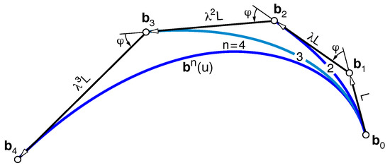
Figure 1. Dimensionless constraints $\left\{\phi ,\lambda \right\}$ characterizing the shape of a typical Bézier curve ${\mathbf{b}}^n\left(u\right)$ (degree $n=2,3,4$).

(i)

Constant supplementary angle $\phi$ between consecutive control legs;

(ii)

Constant ratio $\lambda$ between their lengths.

Regarding the remaining degrees of freedom, ${\mathbf{b}}_0$ determines the position of the curve, whereas $\Delta {\mathbf{b}}_0$ its orientation and size. Therefore, there exist several degree-n curves sharing $\left\{\phi ,\lambda \right\}$, related by a direct similarity ∼, i.e., rigid motions plus uniform dilations [20]. Formally speaking, the set of degree-n typical curves admits a partition into equivalence classes defined by ∼.

We recall that typical curves coincide with segments of a family of offset-rational sinusoidal spirals first introduced in Bézier form by Ueda [21,22] via a pedal-point construction. Later, Sánchez-Reyes [23] identified these spirals as belonging to the special subset of Bézier curves in polar coordinates [24], and Sánchez-Reyes [25] noted that they coincide with typical curves, giving a simple recipe to compute their rational Bézier offsets. Therefore, several remarkable results in [4] come as a direct consequence of these connections.

This paper is organized as follows. First (Section 2), we define the above family of sinusoidal spirals. Next (Section 3), to make the article self-contained, we briefly review their construction by raising a straight line to the nth power in the complex plane, concluding that spiral segments coincide with typical curves. In Section 4, this result allows us to confirm that typical curves contain at most one curvature extremum, namely the vertex [26] of the spiral, and that they form a closed set with respect to the subdivision operation at an arbitrary point. Finding the parameter value at the vertex or the corresponding constraints for each segment after subdivision become straightforward exercises. Finally, in Section 5, conclusions are drawn.

2. Sinusoidal Spirals of Negative Index $-\mathbf{1}/\mathit{n}$

Sinusoidal spirals [27,28,29,30,31], already studied in 1718 by the celebrated mathematician Colin Maclaurin, are planar curves enjoying remarkable optical [32] and kinematic properties [33]. In a suitable system of polar coordinates $(r,\theta )$ with center $\mathbf{O}$ at the so-called pole, a sinusoidal spiral has a polar radius $r\left(\theta \right)={cos}^{1/q}\left(q\theta \right)$, where the rational number $q\in \mathbb{Q}$ is called index [28].

The particular case of a negative reciprocal index $q=-1/n,n\in \mathbb{N}$:

$$r\left(\theta \right)={cos}^{-n}(\theta /n),\theta \in (-\frac{\pi }{2},\frac{\pi }{2})n,$$

(3)

defines a classical subset of degree-n polynomial curves, described by Loria [29] more than a century ago. Aside from the degenerate case of a vertical line $(n=1)$, this family encompasses a parabola with focus at $\mathbf{O}$ $(n=2)$ and the T-cubic $(n=3)$. Curves (3) are symmetric with respect to their axis $\theta =0$, where the vertex $\mathbf{V}$ is located, at unit distance from $\mathbf{O}$.

Since the term spiral usually implies monotonic curvature, each curve in the family ($n\ge 2$) is actually composed of two semi-infinite spiral segments: that corresponding to $\theta \in [0,n\frac{\pi }{2})$, partially plotted in Figure 2, and its mirror image $\theta \in (-n\frac{\pi }{2},0]$. Indeed, their curvature $\kappa \left(\theta \right)$ admits a simple expression [30,34]:

$$\kappa \left(\theta \right)=\frac{n-1}{n}{cos}^{n+1}(\theta /n),$$

(4)

attaining, for $n\ge 2$, a single maximum $\kappa \left(0\right)=\frac{n-1}{n}$ precisely at the vertex $\theta =0$ (Figure 2).

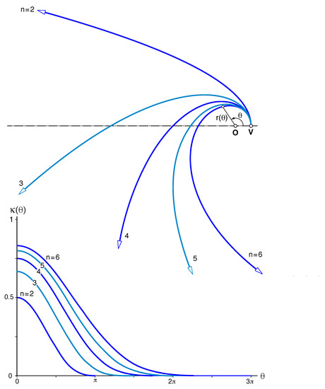
Figure 2. Family of degree-n sinusoidal spirals and their curvature plot $\kappa \left(\theta \right),\theta \in [0,\frac{\pi }{2}n)$.

3. Coincidence between Spiral Segments and Typical Curves

In this section, we recall that degree-n typical curves coincide with sinusoidal spirals. The only difference is how they are expressed: spirals (3) globally in polar coordinates, whereas typical curves as segments in Bézier form. We confirm that any spiral segment is a typical curve by finding its Bézier form and then that any typical curve can be constructed as a spiral segment, aside from direct similarity.

3.1. Construction by Raising a Line to the $nth$ Power in the Complex Plane

The key idea [25] is that a degree-n spiral ${\mathbf{b}}^n\left(\theta \right)$ can be generated by raising to the nth power, in the complex plane, a vertical straight line through the vertex $\mathbf{V}=1$ (on the real axis, at unit distance from the origin $\mathbf{O}$). Parameterizing the line $\mathbf{b}\left(\alpha \right)$ with the fractional polar angle $\alpha =\theta /n$:

$$\mathbf{b}\left(\alpha \right)=\frac{{\mathrm{e}}^{\mathrm{i}\alpha }}{cos\alpha }\stackrel{{\mathbf{z}}^n}{\to }{\mathbf{b}}^n\left(\theta \right)=\frac{{\mathrm{e}}^{\mathrm{i}\theta }}{cos(\theta /n)},\alpha =\theta /n\in (-\frac{\pi }{2},\frac{\pi }{2}).$$

(5)

To generate the segment spanning the angle $\theta \in [{\theta }_0,{\theta }_n]$, consider only the corresponding line segment shown in Figure 3, spanning a polar angle $\alpha \in [{\alpha }_0,{\alpha }_0+\phi ]=[{\theta }_0/n,{\theta }_n/n]$, with endpoints ${\mathbf{z}}_0,{\mathbf{z}}_1$. However, expression (5) furnishes a trigonometric parameterization ${\mathbf{b}}^n\left(\theta \right)$. To obtain a polynomial Bézier form ${\mathbf{b}}^n\left(u\right)$, use, instead, a linear parameter

$$u\left(\alpha \right)=\frac{tan\alpha -tan{\alpha }_0}{tan({\alpha }_0+\phi )-tan{\alpha }_0},u\in [0,1],$$

(6)

and write the line segment in degree-one Bézier form $\mathbf{b}\left(u\right)=(1-u){\mathbf{z}}_0+u{\mathbf{z}}_1$, where

$$\begin{array}{ccc}\hfill & & {\mathbf{z}}_0={\rho }_0{\mathrm{e}}^{\mathrm{i}{\alpha }_0},{\rho }_0=1/cos{\alpha }_0\hfill \\ & & {\mathbf{z}}_1=\mathbf{\lambda }{\mathbf{z}}_0,\mathbf{\lambda }=\lambda {\mathrm{e}}^{\mathrm{i}\phi },\lambda =\frac{cos{\alpha }_0}{cos({\alpha }_0+\phi )}.\hfill \end{array}$$

(7)

Raising $\mathbf{b}\left(u\right)$ to the nth power yields a degree-n curve ${\mathbf{b}}^n\left(u\right)$ whose Bézier points ${\mathbf{b}}_k$ form a geometric progression of common ratio $\mathbf{\lambda }$:

$${\mathbf{b}}_k={\mathbf{\lambda }}^k{\mathbf{b}}_0,k=0,\dots ,n,{\mathbf{b}}_0={\mathbf{z}}_0^n.$$

(8)

This result admits a clear geometric interpretation (Figure 3):

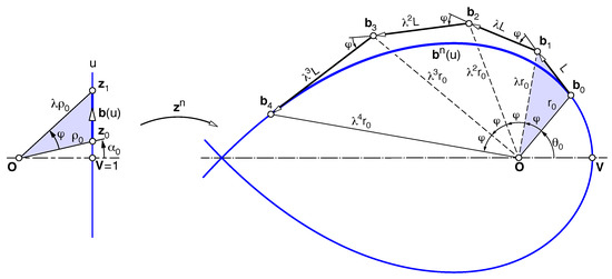
Figure 3. Raising to the nth power a line segment $\mathbf{b}\left(u\right)$ generates a degree-n typical curve ${\mathbf{b}}^n\left(u\right)$, $(n=4)$.

(I)

Each control leg ${\mathbf{b}}_k{\mathbf{b}}_{k+1}$ sees $\mathbf{O}$ with constant angle $\phi$;

(II)

The ratio between polar radii of consecutive points ${\mathbf{b}}_k,{\mathbf{b}}_{k+1}$ is the constant $\lambda$ (7).

Deliberately, we employed symbols $\left\{\phi ,\lambda \right\}$ coinciding with the constraints (2) of a typical curve ${\mathbf{b}}^n\left(u\right)$, because conditions (I), (II) imply those (i), (ii) characterizing typical curves described in the introduction. Indeed, by spiral similarity [20] of center $\mathbf{O}$, with angle $\phi$ and dilation $\lambda$, the triangle $▵\mathbf{O}{\mathbf{b}}_0{\mathbf{b}}_1$ (similar to $▵\mathbf{O}{\mathbf{z}}_0{\mathbf{z}}_1$ and shaded in Figure 3) furnishes the adjacent $▵\mathbf{O}{\mathbf{b}}_1{\mathbf{b}}_2$ and so on. Thus, in the resulting fan with common vertex $\mathbf{O}$, all triangles $▵\mathbf{O}{\mathbf{b}}_k{\mathbf{b}}_{k+1}$ are similar and, consequently, the two constraints (i), (ii) are fulfilled.

Conversely, any typical curve ${\mathbf{b}}^n\left(u\right)$, defined by a pair $\left\{\phi ,\lambda \right\}$, admits a spiral construction (aside from direct similarity). More precisely, our construction can always generate a class representative of the equivalence class, defined in the Introduction, to which ${\mathbf{b}}^n\left(u\right)$ belongs. The required angle ${\alpha }_0$ is that guaranteeing the ratio $\lambda$ (7), hence, obtained by isolation:

$$tan{\alpha }_0=\frac{cos\phi -1/\lambda }{sin\phi }.$$

(9)

3.2. Particular Cases: Vertex at the Endpoint and Symmetric Segments

Figure 4 illustrates the particular case of a spiral segment with an initial Bézier point ${\mathbf{b}}_0=\mathbf{V}$ at the vertex, which results in monotonically decreasing curvature. This special geometry, already considered by Ueda [21] and generated by setting ${\alpha }_0=0$, implies ${\mathbf{z}}_0=\mathbf{V}$, a ratio $\lambda =1/cos\phi$, and right triangles $▵\mathbf{O}{\mathbf{z}}_0{\mathbf{z}}_1\sim ▵\mathbf{O}{\mathbf{b}}_k{\mathbf{b}}_{k+1}$. Since ${\mathbf{b}}_0$ does not depend on n, for a given $\phi$ the control polygon of ${\mathbf{b}}^{n+1}\left(u\right)$ is built incrementally from that of ${\mathbf{b}}^n\left(u\right)$, by adding a new leg ${\mathbf{b}}^n{\mathbf{b}}^{n+1}$.

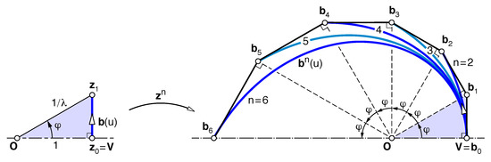
Figure 4. Degree-n typical curves with endpoint ${\mathbf{b}}_0$ at the vertex $\mathbf{V}$, $(n=2,3,4,5,6)$.

Figure 5 illustrates another remarkable case considered in [4], namely symmetric segments, achieved by setting ${\alpha }_0=-\phi /2$. Consequently, $\lambda =1$ and by (7) and (8) all Bézier points lie on a circle, centred at $\mathbf{O}$ and of radius ${\rho }_0^n={cos}^{-n}(\phi /2)$.

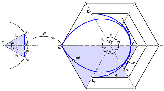
Figure 5. Degree-n symmetric curves $(n=2,4,6)$. The Bézier points lie on a circle ${\mathcal{C}}_n$ centred at $\mathbf{O}$.

4. Properties of Typical Curves

In this section, we employ the above construction in the complex plane to facilitate the study of typical curves. The location of the initial line segment $\mathbf{b}\left(u\right),u\in [0,1]$, an affine image of the domain, determines the constraints $\left\{\phi ,\lambda \right\}$, and then the power function $\mathbf{z}\to {\mathbf{z}}^n$ generates ${\mathbf{b}}^n\left(u\right)$ by stretching $\mathbf{b}\left(u\right)$ and wrapping it around $\mathbf{O}$. Thus, certain properties can be analyzed from the geometry of $▵\mathbf{O}{\mathbf{z}}_0{\mathbf{z}}_1$, where the degree n is immaterial.

4.1. Curvature

In Section 2, we trivially proved that a sinusoidal spiral (3), and hence a typical curve, attains its only one curvature maximum at the vertex $\mathbf{V}$ ($\theta =0$, that is, $\alpha =0$). This result corresponds to Theorem 1 in [4], proved via a detailed analysis of the curvature function.

In [4,5,10], the condition for monotone curvature was derived by analyzing $\kappa \left(u\right)$. Geometrically, this condition reduces to a spiral segment ${\mathbf{b}}^n\left(u\right),u\in [0,1]$ not containing the vertex $\mathbf{V}$, which means a polar angle $\theta \in [{\theta }_0,{\theta }_n]$, and hence a fractional angle $\alpha$ (5), strictly positive or negative. This is equivalent to a segment $\mathbf{b}\left(u\right),u\in [0,1]$ not containing $\mathbf{V}$, i.e., either above or below the real (horizontal) axis in the complex plane. The orientation of $\mathbf{b}\left(u\right)$ determines the curvature behavior: decreasing if $\mathbf{b}\left(u\right)$ moves away from $\mathbf{V}$, and increasing if towards $\mathbf{V}$. These two possibilities are sketched in Figure 6:

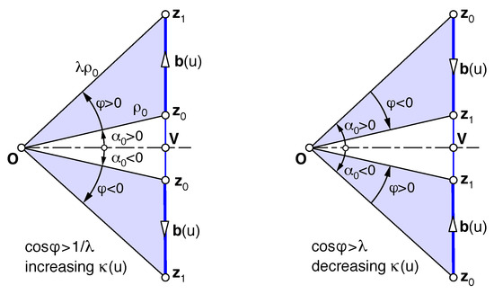
Figure 6. Condition for monotone curvature $\kappa \left(u\right)$: $\mathbf{b}\left(u\right)$ must not contain the vertex $\mathbf{V}$.

• Decreasing $\kappa \left(u\right)$: Since $\mathbf{b}\left(u\right)$ moves away from $\mathbf{V}$, the angles ${\alpha }_0,\phi$ must share their signs. This is tantamount to a positive numerator in the quotient (9), so that $cos\phi >1/\lambda$.
• Increasing $\kappa \left(u\right)$: Reverse the parameterization of $\mathbf{b}\left(u\right)$, by replacing $\left\{\phi ,\lambda \right\}\to \left\{-\phi ,1/\lambda \right\}$. The above condition transforms to $cos\phi >\lambda$.

4.2. Parameter Value u for the Vertex $\mathbf{V}$

To obtain the Bézier parameter u for $\mathbf{V}$, there is neither need to write out the curvature (4) as a function $\kappa \left(u\right)$ of u, find its derivative (already available in [19]) and then its zero, as done in [4,10]. Rather rewrite $u\left(\alpha \right)$ (6) in terms of the ratio $\lambda$, instead of the angle ${\alpha }_0$, by expanding $tan({\alpha }_0+\phi )$ and introducing relationship (9):

$$u\left(\alpha \right)=\frac{1-\lambda cos\phi +\lambda sin\phi tan\alpha }{1-2\lambda cos\phi +{\lambda }^2},u\in [0,1].$$

(10)

Substituting for $\alpha =0$, we obtain the formula in [4], previously derived by Bizzarri et al. [10]:

$$u\left(0\right)=\frac{1-\lambda cos\phi }{1-2\lambda cos\phi +{\lambda }^2}.$$

(11)

As anticipated, $u\left(0\right)$ does not depend on n, since it is determined by the geometry of $▵\mathbf{O}{\mathbf{z}}_0{\mathbf{z}}_1$. In particular, this general expression (11) furnishes the parameter value corresponding to the vertex $\mathbf{V}$ of a parabola $(n=2)$, already given by Choi et al. [35] or by Yan et al. [36] in terms of the control points instead of $\left\{\phi ,\lambda \right\}$.

4.3. Subdivision at an Arbitrary Point

Splitting a spiral at an arbitrary parameter value $\widehat{u}=u\left(\widehat{\alpha }\right)$ (10) generates two segments of the same spiral and trivially two typical curves I and II, with angles ${\phi }^{\mathrm{I}},{\phi }^{\mathrm{II}}$ such that $\phi ={\phi }^{\mathrm{I}}+{\phi }^{\mathrm{II}}$. The subdivision can be performed in a simple way without invoking the standard de Casteljau algorithm. Split $\mathbf{b}\left(u\right)$ at $\widehat{u}$, which yields the respective angles (Figure 7)

$${\alpha }_0^{\mathrm{I}}={\alpha }_0,{\phi }^{\mathrm{I}}=\widehat{\alpha }-{\alpha }_0,{\alpha }_0^{\mathrm{II}}=\widehat{\alpha },{\phi }^{\mathrm{II}}=\phi -{\phi }^{\mathrm{I}}.$$

(12)

These values, in turn, furnish the corresponding ratios ${\lambda }^{\mathrm{I}},{\lambda }^{\mathrm{II}}$ via (7) and the control points as the geometric progression (8). Once again, the degree n plays no role.

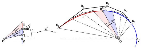
Figure 7. Subdividing a typical curve ($n=4$) at an arbitrary parameter value $\widehat{u}=u\left(\widehat{\alpha }\right)$.

He et al. [4] considered only the case of subdivision at $\mathbf{V}$, analytically proving that the resulting segments are still typical curves by confirming that, in characterization (1), the transformation matrices for each segment [6] express rotation plus uniform dilation. This special case $\widehat{\alpha }=0$ results in particular ratios (7):

$${\lambda }^{\mathrm{I}}=cos{\phi }^{\mathrm{I}};{\lambda }^{\mathrm{II}}=1/cos{\phi }^{\mathrm{II}},$$

and segments I, II display the geometry of Figure 4 (or its mirror).

5. Conclusions

Degree-n typical Bézier curves amount to segments of a classical family of sinusoidal spirals, of negative index $-1/n$, an elucidating relationship overlooked in the literature. Sinusoidal spirals are defined globally in polar coordinates, whereas typical curves are written as segments in Bézier form. This connection provides a deeper geometric insight into typical curves and makes their analysis for CAGD purposes notably simpler. As trivial consequences, they display at most a curvature extremum (the vertex), and subdividing a curve at an arbitrary point furnishes two typical curves.

Unsurprisingly, complex arithmetics facilitates the construction of typical curves, as usual with offset-rational curves. Any degree-n typical curve ${\mathbf{b}}^n\left(u\right)$ (aside from direct similarity) can be generated by raising to the nth power a linear segment $\mathbf{b}\left(u\right)$ in Bézier form, lying on a vertical line through the vertex. Thus, finding the parameter value for the vertex amounts through straightforward trigonometry. The complex power function $\mathbf{z}\to {\mathbf{z}}^n$ stretches $\mathbf{b}\left(u\right)$ and wraps it around the origin to create ${\mathbf{b}}^n\left(u\right)$, whose Bézier points form a (complex) geometric progression.

As one of the reviewers kindly observed, future work could be aimed at applying this complex power construction, along with subdivision, to find tight bounds of the spiral segments, improving those provided by spiral fat arcs [37]. Such bounds speed up curve–curve intersection, a fundamental task in geometry processing. The control polygon, connecting points ${\mathbf{b}}_k$ (8) evenly spaced by the polar angle $\phi$, furnishes an outer bounding polyline, whereas successive chords, connecting points on the spiral evenly spaced by the angle $\phi$, could provide an inner bound.

References

- Levien, R.; Séquin, C. Interpolating Splines: Which is the fairest of them all? Comput.-Aided Des. Appl. 2009, 6, 91–102. [Google Scholar] [CrossRef]
- Yoshida, N.; Saito, T. Interactive aesthetic curve segments. Vis. Comput. 2006, 15, 879–891. [Google Scholar] [CrossRef]
- Meek, M.; Walton, D.J. The use of Cornu spirals in drawing planar curves of controlled curvature. J. Comput. Appl. Math. 1989, 25, 69–78. [Google Scholar] [CrossRef][Green Version]
- He, C.; Zhao, G.; Wang, A.; Li, S.; Cai, Z. Planar typical Bézier curves with a Single Curvature Extremum. Mathematics 2021, 9, 2148. [Google Scholar] [CrossRef]
- Mineur, Y.; Lichah, T.; Castelain, J.M.; Giaume, H. A shape controled fitting method for Bézier curves. Comput. Aided Geom. Des. 1998, 15, 879–891. [Google Scholar] [CrossRef]
- Farin, G. Class A Bézier curves. Comput. Aided Geom. Des. 2006, 15, 573–581. [Google Scholar] [CrossRef]
- Mineur, Y. A Shape Constrained Curve Approximation Method for Styling Surfaces Modeling. In Proceedings of the Posters Papers proceedings of WSCG’ 2003, 11th International Conference in Central Europe on Computer Graphics, Visualization and Computer Vision’ 2003, Plzen, Czech Republic, 3–7 February 2003. [Google Scholar]
- Higashi, M.; Kaneko, K.; Hosaka, M. Generation of high quality curve and surface with smoothing varying curvature. In Eurographics’88: Proceedings of the European Computer Graphics Conference and Exhibition; Duce, D.A., Jancene, P., Eds.; Elsevier Science: Amsterdam, The Netherlands, 1988; pp. 79–92. [Google Scholar]
- Higashi, M. High-quality solid-modelling system with free-form surfaces. Comput.-Aided Des. 1993, 25, 172–183. [Google Scholar] [CrossRef]
- Bizzarri, M.; Lávička, M.; Vršek, J. Note on planar Pythagorean hodograph curves of Tschirnhaus type. Comput. Aided Geom. Des. 2021, 89, 102022. [Google Scholar] [CrossRef]
- Farouki, R.T. Pythagorean-Hodograph Curves: Algebra and Geometry Inseparable; Springer: Berlin, Germany, 2008. [Google Scholar]
- Farouki, R.T.; Giannelli, C.; Sestini, A. New Developments in Theory, Algorithms, and Applications for Pythagorean–Hodograph Curves. In Advanced Methods for Geometric Modeling and Numerical Simulation; Giannelli, C., Speleers, H., Eds.; Springer: Cham, Switzerland, 2019; pp. 127–177. [Google Scholar]
- Hoffmann, C.M.; Peters, J. Geometric constraints for CAGD. In Mathematical Methods for Curves and Surfaces; Daehlen, M., Lyche, T., Schumaker, L.L., Eds.; Vanderbilt University Press: Nashville, TN, USA, 1995; pp. 237–253. [Google Scholar]
- Meek, M.; Walton, D.J. Geometric Hermite interpolation with Tschirnhausen cubics. J. Comput. Appl. Math. 1997, 81, 299–309. [Google Scholar] [CrossRef]
- Meek, M.; Walton, D.J. Hermite interpolation with Tschirnhausen cubic spirals. Comput. Aided Geom. Des. 1997, 14, 619–635. [Google Scholar] [CrossRef]
- Byrtus, M.; Bastl, B. Hermite interpolation by PH cubics revisited. Comput. Aided Geom. Des. 2010, 27, 622–630. [Google Scholar] [CrossRef]
- Farouki, R.T.; Peters, J. Smooth curve design with double-Tschirnhausen cubics. Annals Num. Math. 1996, 3, 63–82. [Google Scholar]
- Bastl, B.; Slabá, K.; Byrtus, M. Planar C1 Hermite interpolation with uniform and non-uniform TC-biarcs. Comput. Aided Geom. Des. 2013, 30, 58–77. [Google Scholar] [CrossRef]
- Cantón, A.; Fernández-Jambrina, L.; Vázquez-Gallo, M.J. Curvature of planar aesthetic curves. J. Comput. Appl. Math. 2021, 381, 113042. [Google Scholar] [CrossRef]
- Coxeter, H.S.M.; Greitzer, S.L. Geometry Revisited; The Mathematical Association of America: Washington, DC, USA, 1967. [Google Scholar]
- Ueda, K. A Sequence of Bézier Curves Generated by Successive Pedal-Point Constructions. In Curves and Surfaces with Applications in CAGD; Le Méhauté, A., Rabut, C., Schumaker, L.L., Eds.; Vanderbilt University Press: Nashville, TN, USA, 1997; pp. 427–434. [Google Scholar]
- Ueda, K. Pedal Curves and Surfaces. In Mathematical Methods in CAGD: Oslo 2000 (Innovations in Applied Mathematics); Lyche, T., Schumaker, L.L., Eds.; Vanderbilt University Press: Nashville, TN, USA, 2001; pp. 497–506. [Google Scholar]
- Sánchez-Reyes, J. p-Bézier curves, spirals, and sectrix curves. Comput. Aided Geom. Des. 2002, 19, 445–464. [Google Scholar] [CrossRef]
- Sánchez-Reyes, J. Single-valued curves in polar coordinates. Comput.-Aided Des. 1990, 22, 19–26. [Google Scholar] [CrossRef]
- Sánchez-Reyes, J. Offset-rational sinusoidal spirals in Bézier form. Comput. Aided Geom. Des. 2007, 24, 142–150. [Google Scholar] [CrossRef]
- Gray, A.; Abbena, E.; Salomon, S. Modern Differential Geometry of Curves and Surfaces with Mathematica, 3rd ed.; Chapman & Hall/CRC: Boca Raton, FL, USA, 2006. [Google Scholar]
- Lawrence, J.D. A Catalog of Special Plane Curves; Dover: New York, NY, USA, 1972. [Google Scholar]
- Yates, R.C. Curves and Their Properties; The National Council of Teachers of Mathematics: Reston, VA, USA, 1974. [Google Scholar]
- Loria, G. Spezielle Algebraische und Transzendente Ebene Kurven: Theorie und Geschichte; Teubner: Leipzig, Germany, 1911. [Google Scholar]
- Gomes Teixeira, F. Traité des Courbes Spéciales, Remarquables Planes et Gauches, Tome II; Reprinted by Éditions Jacques Gabay: Paris, France, 1909. [Google Scholar]
- Shikin, E. Handbook and Atlas of Curves; CRC Press: Boca Raton, FL, USA, 1995. [Google Scholar]
- Weiss, G.; Martini, H. On Curves and Surfaces in Illumination Geometry. J. Geom. Graph. 2000, 2, 169–180. [Google Scholar]
- Kuczmarski, F. Rolling Sinusoidal Spirals. Amer. Math. Monthly 2012, 119, 451–467. [Google Scholar] [CrossRef]
- Rutter, J.W. Geometry of Curves; Chapman & Hall/CRC: Boca Raton, FL, USA, 2000. [Google Scholar]
- Choi, J.W.; Curry, R.E.; Elkaim, G.H. Minimizing the maximum curvature of quadratic Bézier curves with a tetragonal concave polygonal boundary constraint. Comput.-Aided Des. 2012, 44, 311–319. [Google Scholar] [CrossRef]
- Yan, J.; Schiller, S.; Wilensky, G.; Carr, N.; Schaefer, S. κ-Curves: Interpolation at Local Maximum Curvature. ACM Trans. Graph. 2017, 36, 1–7. [Google Scholar] [CrossRef]
- Bartoň, J.; Elber, G. Spiral fat arcs—Bounding regions with cubic convergence. Graph. Models 2011, 73, 50–57. [Google Scholar] [CrossRef]
Publisher’s Note: MDPI stays neutral with regard to jurisdictional claims in published maps and institutional affiliations. |
© 2021 by the author. Licensee MDPI, Basel, Switzerland. This article is an open access article distributed under the terms and conditions of the Creative Commons Attribution (CC BY) license (https://creativecommons.org/licenses/by/4.0/).