Article

Probability Models of Distributed Proof Generation for zk-SNARK-Based Blockchains

1
Bogolyubov Institute for Theoretical Physics, 03143 Kiev, Ukraine
2
Horizen, 20121 Milan, Italy
3
IOHK Research, Hong Kong
4
Department of Information Security, Zaporizhzhia Polytechnic National University, 69063 Zaporizhzhia, Ukraine
*
Authors to whom correspondence should be addressed.
Mathematics 2021, 9(23), 3016; https://doi.org/10.3390/math9233016
Submission received: 26 October 2021 / Revised: 16 November 2021 / Accepted: 18 November 2021 / Published: 24 November 2021
(This article belongs to the Special Issue Advances in Blockchain Technology)

Abstract

:
The paper is devoted to the investigation of the distributed proof generation process, which makes use of recursive zk-SNARKs. Such distributed proof generation, where recursive zk-SNARK-proofs are organized in perfect Mercle trees, was for the first time proposed in Latus consensus protocol for zk-SNARKs-based sidechains. We consider two models of a such proof generation process: the simplified one, where all proofs are independent (like one level of tree), and its natural generation, where proofs are organized in partially ordered set (poset), according to tree structure. Using discrete Markov chains for modeling of corresponding proof generation process, we obtained the recurrent formulas for the expectation and variance of the number of steps needed to generate a certain number of independent proofs by a given number of provers. We asymptotically represent the expectation as a function of the one variable n / m , where n is the number of provers m is the number of proofs (leaves of tree). Using results obtained, we give numerical recommendation about the number of transactions, which should be included in the current block, idepending on the network parameters, such as time slot duration, number of provers, time needed for proof generation, etc.

1. Introduction

Sidechains (SCs) [1,2,3,4], and also some similar tools, such as [5,6] are very suitable and prospective instrument in modern blockchains. They may be considered as some adjunct to the blockchain which allows one to obtain some additional features that are not implemented in initial blockchain (which is also called mainchain, not to be confused with sidechain).
Generally speaking, SCs may use an arbitrary consensus protocol with proved security—taking into account conditions in which its security was proved [7,8,9,10]. In what follows we will consider only SCs based on Latus Consensus Protocol [11], which isa hybrid PoS based on Ouroboros Praos [12], with additional binding to a PoW mainchain (MC). Binding to MC is a necessary requirement for SCs [1,2,3,4,11], to guarantee such blockchain properties as liveness and persistence [13]. To ensure security level of transactions in SC, some information should be regularly sent from SC to MC. One MC may have a plethora of SCs, so we need to reduce the volume of information sent, but in a such way that will not increase different risks for SC. In Latus consensus, this information contains a series of recursive zk-SNARK-proofs [14,15] that establish decentralized and verifiable cross-chain data transfers.
The abbreviation “zk-SNARK” means “zero-knowledge Succinct Non-interactive ARgument of Knowledge” [16]. This is a really ingenious technique for proving that somebody knows some information without revealing anything about this information, or for proving that some statement is true, without revealing its details. zk-SNARK may be considered as some kind of non-interactive zero-knowledge proof system, which was introduced about 40 years ago in [17] and has been intensively developing since then. For the first time term “zk-SNARK” itself was introduced in [18], based on [19]. In [20,21] the Pinoccio protocol was introduced, making zk-SNARKs more convenient and applicable for general purposes.
As it was mentioned, zk-SNARK is succinct argument, which means that the proof length is sufficiently small. For example, it may be constant, as in [22], i.e., its length depends only on the desirable security level and does not depend on the size of data which we prove to be true. That is why zk-SNARKs are a very attractive tool to be used in blockchains, where the problem of block size reduction is imminent. They are used, for example, in blockchains such as zCash [23], MINA [24], and Horizen [11], and even some special cryptographic primitives, like block ciphers and hash-functions, are created for using in zk-SNARKs [25,26].
Each blockchain choses variant of zk-SNARK, which is most suitable for it. Latus Consensus uses Darlin [27], which is advanced composition of Marlin [28] and Halo [29].
This work does not deal with developing of zk-SNARK topic, and, actually, for our investigations it does not matter what exactly zk-SNARK is used for in Latus. Similar to [1,2,3,4], it is devoted to providing of stable and correct functioning of SCs. However, unlike these works, we investigate these issues within each separate block, because block creation in Latus is a rather cumbersome procedure. In Latus, decentralized proofs generation use a special dispatching scheme, which allows all interested parties, or provers, to create a randomly chosen proof and then to submit it to the blockchain, getting some reward (incentive) for each accepted proof. If two or more provers created the same proof, blockforger (the entity who creates block) chooses one of them. In other words, Latus Consensus allows all interested parties to participate simultaneously in one-block generation. From the one hand, it increases decentralization; the need to create more complicated protocols of interaction between blockforger and provers, as well as the choice parameters of these protocols and justification of their correctness and robustness. The article is devoted just to these questions.
In Latus, decentralized proofs generation use a special dispatching scheme, which allows all interested parties, or provers, to create a randomly chosen proof and to then submit it to the blockchain, getting some reward (incentive) for each accepted proof. If two or more provers created the same proof, blockforger (the entity who creates block) chooses one of them.
The main feature of the Latus consensus is to reduce the volume of information sent to MC from SC, using a recursive composition of zk-SNARKs, which allows to construct a succinct proof of the correctness for sidechain state transitions for the period of a withdrawal epoch. At the end of an epoch, a zk-SNARK for a withdrawal certificate is constructed to prove correctness of sidechain state transitions for the whole epoch and validates backward transfers. Such a procedure allows the MC to efficiently verify the sidechain’s activity, without using any intermediary—such as certifiers [4]—and without delving into the details of the processes inside SC.
In SC, a blockforger collects the transactions he intends to include in his block, orders them and forms correspondent proposals for provers. Each block contains some totally ordered set of transactions (its size is the power of 2) and perfect binary tree, which nodes are zk-SNARK-proofs. In what follows we will call this tree “proof tree”. Each proof of the bottom of the tree proves some assertion about the correctness of transition from some state of UTXO (unspent transaction output) to its next state, which is the state after corresponding transaction. Such assertions we will call “base assertions”, and proofs of the bottom level, which are the leaves of the proof tree, we will call “base proofs”. Other, internal nodes of the proof tree are so-called “merge” proofs [4], which prove the correctness of two proofs in child nodes. Therefore proof in the root node proves correctness of transitions between UTXO states corresponding to the whole block.
All zk-SNARK-proofs for the proof tree are distributively constructed by proovers. Each prover, who creates zk-SNARK-proof, assigns the prices for his proofs within some interval or set, defined at the end of the previous epoch. If there is more than one proof for some node of the proof tree, the blockforger chooses the cheapest one. Under these conditions, the mutual activity of blockforger and provers should provide efficient and stable functioning of sidechain.
This work is a revised, corrected, and extended version of the conference thesis [30]. It contains the results which describe and explain the functioning of SCs, and first of all the blockforger’s and prover’s behavior, using probability theory and combinatorial apparatus. We use Markov chains for modeling distributed proof generation process in zk-SNARKs-based blockchains. The main purposes of our researches are:
  • To estimate the number of steps (or to find its expectation and variance) needed to build a complete set of zk-SNARK-proofs for base assertions corresponding to the transactions, which the blockforger includes in the block he creates;
  • Using these results, to recommend the maximal number of transactions that the blockforger should include in the block, to guarantee that the corresponding proof tree will be created with high probability during one time slot.
We consider two different models, which corresponds to two types of proof construction. The first model describes the the simpler case when all the proofs are built independently (like one level of the proof tree). The second model investigates a more complicated problem, when the proofs are located at nodes from the different levels of the proof tree. Such a set of proofs has the natural partial order, because the proofs from the upper level of the tree may be constructed only when the proofs from the previous levels are constructed.
The paper is organized as follows. At the beginning of the Section 2 we give some preliminary information from combinatorics, probability theory, and Markov chains technique, which is necessary for further researches. The notion of lumping for Markov chains is a special case regarding the general idea of factorization for mathematical structures. Unfortunately only a small part of textbooks pay attention to this concept. Our point of view here is that a problem can be described by several Markov chains with different level of factorization, depending on how many details we want to know at the moment. In Section 2.3 we illustrate this idea on the sample of coupon collector’s problem.
Then, in Section 3 we analyse the number of steps needed to construct a complete set of proofs, which are the leaves of the unproved part of the proof tree. In this case they may be generated independently and simultaneously. We give a series of examples of different stochastic models, which are helpful in our researches. We prove that two models, described in Examples 5 and 6, are stochastically equivalent, although the first one was initially formulated as non-Markovian, and the second one was formulated in terms of the Markov chain. We study the lumped form of this model in Example 7. Using this technique we obtained the recurrent formulas for the expectation and variance of the number of steps, depending on the number of provers n and the number of leaves m, and then asymptotically reduce the expectation to a function h of single parameter n / m and describe its behavior.
Finally in Section 4 we research the process of proof creation for the entire perfect binary tree and show that this construction is convenient to generalize the previously investigated models for the case of a partially ordered set. Some useful insights emerged from this generalization, such as a more appropriate probability distribution on poset items. We conclude our article with Section 4.6 which contains numerical results regarding the number of transactions, which the blockforger should include in the current block. Such a number depends on the network parameters, such as time slot duration, number of active provers, time needed for prove generation, and so on. We present a few tables with these recommended numbers of transactions for the different preset probabilities of successful block generation.

2. Preliminaries

Here we provide the necessary facts about lumping for Markov chains and describe the Markov chain corresponding to the coupon collector problem as a result of two subsequent lumping constructions. These technique and examples are important for our main models.
Notation 1.
For cardinality of finite set S, we use two notations (depending on convenience):
# S = | S | .
Notation 2.
For non-negative integer m, by the corresponding boldface letter m we denote (depending on context) the totally ordered poset { 1 < 2 < < m } or its underlying set { 1 , 2 , , m } .
Notation 3.
Iverson bracket for statement P turns boolean value into the corresponding number:
[ [ P ] ] : = 1 , i f   P   i s   t r u e , 0 , i f   P   i s   f a l s e .
Notation 4.
We use the generally accepted notations for
  • falling factorials:
    n r ̲ = ( n ) r = n ( n 1 ) ( n r + 1 ) ;
  • binomial and multinomial coefficients:
    m k : = m ! k ! ( m k ) ! ; m m 1 , , m n : = m ! m 1 ! m n ! , where m 1 + + m n = m .

2.1. Stirling Numbers of the Second Kind

The “twelve-fold way” of combinatorics ([31], 1.9) counts the number of mappings (injections, surjections, or all possible) between two finite sets, distinguishing or not distinguishing elements in each of them. For example, the symmetric groups S m and S n act on the set Sur ( m , n ) of surjections m n via pre- and post- composition, respectively. The Stirling partition numbers (or Stirling numbers of the second kind) can be defined as a number of orbits:
S ( m , n ) = m n : = | S n Sur ( m , n ) | ,
i.e., this is the number of partitions of the m labeled elements into n non-empty non-labelled blocks, or the number of ways to nest m Matryoshka dolls so you can still see n (matryoshkas are linear, ordered by size).
The action S n on Sur ( m , n ) is free, so
| Sur ( m , n ) | = n ! m n .
On the other hand, given a surjection π : m n , elements of the orbit π S m are identified with cosets from S m / St π = S m / ( S m 1 × × S m n ) , where m i = # π 1 ( i ) . All surjections can be calculated via the sum over n-compositions of m:
n ! m n = | Sur ( m , n ) | = m 1 + + m n = m m 1 , , m n 1 S m S m 1 × × S m n = m 1 + + m n = m m 1 , , m n 1 m m 1 , , m n .
Multiplying both parts of (2) by z m / m ! and taking the sum over m one can obtain the exponential generating function for n ! m n
m = 0 n ! m n z m m ! = ( e z 1 ) n .
Each map f : m n is factorised as f = ( m Im f n ) . Then the total number of functions m n
n m = S n | S | ! m | S | = r = 0 n m r ( n ) r .
One can consider (4) as an identity between integer polynomial in a free variable n. So we get an alternative definition of Stirling numbers as coefficients of the transition matrix between two polynomial bases.
Möbius inversion [31] (3.7) in the case of power-set P m admits a simpler formulation as the inclusion-exclusion principle [31] (2.1). It allows, on the contrary to (4), to express the number of surjections in terms of the numbers of all functions:
n ! m n = S n ( 1 ) n | S | | S | m = r = 0 n ( 1 ) r n r ( n r ) m .
The (forward) difference operator acts on numerical sequences ( x k ) as Δ : x k x k + 1 x k . Its powers are expressed by binomial formula Δ n x k = r = 0 n ( 1 ) r n r x k + n r . It allows to rewrite the previous formula (5) as:
n ! m n = Δ n 0 m = Δ n k m | k = 0 .
Stirling numbers of the second kind appear in [32] as a double sequence A008277, where one can find some additional information, references, and links.

2.2. Factorisation of Markov Chains

In what follows, we assume that Markov chains are discrete-time, time-homogeneous and with finite or countable state-space S. Elements of transition matrix p are written as
p i j = p ( i , j ) = Pr ( X ( n + 1 ) = j X ( n ) = i ) , i , j S .
A such position of indexes corresponds to the right action of p on the row vector of states. This is a right stochastic matrix, i.e., with j S p i j = 1 .
Here we consider the notion of lumping for Markov chains; see, for example [33] (§6.3). The general mathematical idea of transferring a structure from a set to a factor-set also works in the case of Markov chains. Given a surjection π : S T , consider the corresponding logical matrix v π and its Moore–Penrose inverse v π (see [34]).
v π : = ( δ π ( s ) , t ) s S , t T , v π : = ( v π t v π ) 1 v π t .
In our special case: the logical matrix corresponding to surjection isa projection and, hence, Moore–Penrose inverse v π is a real one-side inverse: v π v π = 1 .
Lemma 1.
Let p = ( p s s ) s , s S be a right stochastic matrix over a state-space S. For surjection π : S T the following conditions are equivalent:
1.
for any t T the sum s π 1 ( t ) p s s is locally constant on s π 1 ( t ) for each t T ;
2.
v π v π p v π = p v π .
Definition 1.
Let p = ( p s s ) s , s S be a right stochastic matrix over a state-space S. A surjection π : S T satisfying the conditions of the previous lemma is called a lumping map (and the corresponding partition S = t T π 1 ( t ) is called lumpable).
Proposition 1.
Let p = ( p s s ) s , s S be a stochastic matrix and π : S T a lumping map.
1.
Then, one can define a new stochastic matrix p π over a state-space T with entries
p t t π : = s π 1 ( t ) p s s , s π 1 ( t ) .
2.
The lumped k-fold transition matrix can be written as
( p π ) k = ( v π p v π ) k = v π p k v π .
We believe that the following statement is a kind of “folkloric” result.
Proposition 2.
Suppose that a finite group G acts on the set of states S by the rule S × G ( s , g ) s g S and the stochastic matrix p = ( p ( s , s ) ) s , s S is G-invariant, i.e.,
p ( s 1 g , s 2 g ) = p ( s 1 , s 2 ) , s 1 , s 2 S , g G .
Then, the canonical projection π : S S / G to the set of orbits is a lumping map.
Proof. 
Denote St s : = { g G s g = s } the stabilizer subgroup of state s. For an orbit s G : = { s g g G } the sum from Lemma 1 takes the form
s π 1 ( s G ) p ( s 1 , s ) = 1 | St s | g G p ( s 1 , s g ) .
Then, the standard argument shows that the last sum is G-invariant as a function on s 1 :
g G p ( s 1 h , s g ) = g G p ( s 1 , s g h 1 ) = g G p ( s 1 , s g ) .

2.3. Coupon Collector Model via Products and Factorizations

The classical coupon collector problem can be described as follows.
Example 1.
There are n distinct coupons in the urn. A collector draws with return one random coupon in a step. The subjects of interest are the following random variables:
  • The number of distinct coupons selected after m steps;
  • The number of steps required to obtain exactly r distinct coupons.
Crossed products of Markov chains (and their generalizations) are described in [35]. We obtain a version of the coupon collector model as the crossed power of a simple deterministic process. The other two versions are results of its subsequent factorizations. It leads to the classical occupancy distribution described via Stirling partition numbers. This context is closely related to our further models.
Example 2
(Hyperoctant-full information). Consider a fully deterministic Markov chain that counts natural numbers: X 0 = 0 , X 1 = 1 , X 2 = 2 , Its transition matrix is a semi-infinite Jordan cell:
J = 0 1 0 0 0 0 1 0 0 0 0 1 .
The n-th crossed power of the above Markov chain has the set of states Z 0 n and transition matrix
p = 1 n i = 1 n 1 Z 0 1 Z 0 i 1 J 1 Z 0 1 Z 0 n i ,
where 1 Z 0 is the identity matrix on the basis Z 0 .
This is a random walk over the n-dimensional hyperoctant Z 0 n with nonzero transition probabilities
p ( a , a + e i ) = 1 / n , a Z 0 n , e i = ( 0 , , 0 i 1 , 1 , 0 , , 0 n i ) .
Then nonzero entries of m-fold transition matrix are
p m ( a , a + h ) = n m m h 1 , , h n , where h i 0 and h 1 + + h n = m .
So each row of this matrix represents a multinomial distribution on vectors h.
The next step is when a collector wants to remember whether each fixed coupon was drawn, no matter how many times.
Notation 5.
For a Z 0 N or a { 0.1 } N the support of a is defined as follows.
supp a : = { i N a i 0 } .
Example 3
(Hypercube-partial information). Iverson bracket (1) applied to each coordinate ( a i ) i n ( [ [ a i > 0 ] ] ) i n gets a lumping map Z 0 n { 0 , 1 } n for the previous Markov chain. According to (7) for the obtained Markov chain on the hypercube { 0 , 1 } n m-step transition matrix p m is the following: if p m ( a , b ) > 0 then a i b i for all i; and by inclusion-exclusion principle
p m ( a , b ) = n m m 1 + + m n = m m 1 , , m n 0 m i > 0 i supp b i supp a m i > 0 m m 1 , , m n = n m r = | supp a | | supp b | ( 1 ) supp | b | r | supp ( b a ) | r | supp a | r m .
In particular,
p m ( a , a ) = ( | supp a | / n ) m , p m ( 0 , b ) = n m | supp b | ! m | supp b | .
If the collector is able to keep only one number in memory, we continue the lumping.
Example 4
(Only number of samples). The projection of hypercube to the main diagonal
{ 0 , 1 } n { 0 , 1 , , n } , ( a i ) 1 i n i a i
is a lumping map. Combining the states, we get so called coupon collecting Markov chain [36] (2.2), where nonzero m-step transition probabilities are the following:
p m ( k , k + r ) = n m n k r s = 0 r ( 1 ) r s r s ( k + s ) m .
The number ξ m = ξ 0 p m of distinct coupons selected after m steps has the classical occupancy distribution [37]:
Pr ( ξ m = r ) = p m ( 0 , r ) = ( n ) r n m m r .
The expectation of number ζ r n of steps required to obtain exactly r distinct coupons is described via harmonic numbers H n = 1 + 1 / 2 + + 1 / n :
E ζ r n = n ( H n H n r ) .

3. Distributed Generation of Sets of Proofs

This section presents the main results about the distributed generation of sets of separate independent proofs. This is the simplified model, where all proofs may be generated simultaneously and independently. This model corresponds, in particular, to the case of the generation of proofs which are on the same level as proof tree.

3.1. Models of Distributed Generation of Sets of Proofs

The further two examples show two possible approaches to the description of this model, which then appear equivalent.
Example 5
(States are subsets). Let provers be special nodes in the peer-to-peer network. They need to construct zk-SNARK-proofs for finite set N of so called proof-candidates.
We describe this process as a Markov chain, whose states are subsets of N N of proof-candidates not yet proved. The number of provers m > 0 is fixed. On each step, beginning in the state N , each prover independently and with equal probabilities selects a single proof-candidate from N and construct its proof, so the selection is given by a function g : m N uniformly distributed among all functions m N . The resulting state is the difference N : = N Im g obtained by removing just the proved elements. Nonzero transition probabilities p ( N , N ) equal the part of all functions m N which come from surjections to N N i.e., g = m N N N .
p ( N , N ) = | Sur ( m , N N ) | | N | m = | N N | ! | N | m m | N N | , N N .
An alternative way is to define a probability measure on trajectories:
Notation 6.
A linear ordering of a set N is a bijection σ : N { 1 , 2 , , | N | } . Denote Ord N the set of linear orderings on N.
Example 6
(Non-Markovian model). Let at the beginning each prover for 1 i m independently select its own so-called priority ordering σ i Ord N with equal probability 1 / | Ord N | = 1 / | N | ! . This determines the chain of states, i.e., the subsets together with linear orderings:
N = N 0 N 1 N k 1 N k = , σ i ( j ) Ord ( N j ) , σ i ( 0 ) = σ i , 1 i m , 0 j k .
In jth step, 1 j k , being in the state N j 1 ith prover select proof-candidate according to the function g j : m N j 1 given by g j ( i ) : = σ i ( j 1 ) 1 ( 1 ) . The next state is N j = N j 1 Im ( g j ) . There is the natural projection ρ N N : Ord ( N ) Ord ( N ) , which removes elements of N N from an ordering. Then, we put
σ i ( j ) = ρ N j N ( σ i ) .
Proposition 3.
The models from Examples 5 and 6 are stochastically equivalent.
Proof. 
We give a sketch of the proof. A more general situation is described in Example 12. Selections of ( σ i ) 1 i m are uniformly distributed on ( Ord N ) m . This implies
  • uniform distribution of g j in the set of functions m N j 1 , and
  • uniform distribution of σ i ( j ) Ord ( N j ) .
The second item follows from the definition (11) and from the fact that the fiber of ρ N N over each point has the same cardinality | Ord N | / | Ord N | = | N | ! / | N | ! . □
Example 7
(States are numbers). The cardinality function N | N | is a lumping map for the Markov chain from Example 5. The states of the factorized Markov chain are { 0 , 1 , , | N | } , the only nonzero elements of transition matrix are the following:
p ( 0 , 0 ) = 1 , p ( n , n r ) = 1 n m n r r ! m r = ( n ) r n m m r , n > 0 , 1 r m .
Note that each row this matrix coincides with the classical occupancy distribution from Example 4.
Let the initial state be ξ 0 m n n . The evolution is described via powers of transition matrix:
ξ k m n = ξ 0 m n p k .
The absorbing state is 0. All trajectories are strictly decreasing and ξ k m n 0 for k n .
The absorption time τ m n is a random variable which measures the exact number of steps m provers needs to generate all n proofs. i.e., τ m n = k + 1 iff ξ k + 1 m n = 0 and ξ k m n 0 .
Taking into account the lower triangular form of our transition matrix, we get recurrent and explicit formulas for probabilities:
Pr ( τ m n = 0 ) = δ n 0 , Pr ( τ m n = k + 1 ) = r = 1 min ( m , n ) p n n r Pr ( τ m n r = k ) = r = 0 min ( m , n ) ( n ) r n m m r Pr ( τ m n r = k )
Pr ( τ m n = k ) = 0 < n k < < n 2 < n 1 = n p n 1 n 2 p n k 1 n k p n k 0 = 0 < n k < < n 2 < n 1 = n n ! ( n 1 n 2 n k ) m m n 1 n 2 m n k 1 n k m n k = r 1 + + r k = n r 1 , , r k > 0 n ! ( r 1 ( r 1 + r 2 ) n ) m m r 1 m r k = s 1 + , s 2 k = n s 1 , s 3 , , s 2 k 1 0 s 2 , s 4 , , s 2 k > 0 n s 1 , , s 2 k ( 1 ) s 1 + s 3 + + s 2 k 1 ( s 2 s 4 s 2 k ) m ( ( s 1 + s 2 ) ( s 1 + s 2 + s 3 + s 4 ) n ) m .
Multiplying (13) by k and taking a sum over k we get the recurrent formula for th moment:
E ( τ m n 1 ) = r = 1 min ( n , m ) p m n r E ( τ m n r ) .
In particular, this allows one to get the next formulas for calculating expectation and variance.
Proposition 4.
Let m > 0 . Then τ m 0 0 and for n > 0
E τ m n = 1 + r = 1 min ( n , m ) ( n ) r n m m r E τ m n r , E ( τ m n ) 2 = 1 + 2 E τ m n + r = 1 min ( n , m ) ( n ) r n m m r E ( τ m n r ) 2 , Var τ m n = E ( τ m n ) 2 ( E τ m n ) 2 .
In Table 1 at the end of the paper we present probability distributions of τ m n accurate to 10 6 (except of the last column). A cell contains the list of pairs k ; p k m n of value k and the corresponding probability p k m n (nonzero up to accuracy). The number of proofs n runs through powers of 2, which corresponds to the number of leaves of a perfect binary tree.
We compare the values of E τ m n as results of infinite-precision calculations according (15) using Wolfram Mathematica and of 10 5 random tests written on C++ of model from Example 6. For m , n { 10 , 20 , 30 , 40 , 50 , 100 , 200 , 300 } the numerical results obtained by these two different ways match up to 2 digits after the dot.
Remark 1.
For fixed positive integer m we consider two modifications of the coupon collector model from Example 4:
1.
After m, 2 m , 3 m , steps all coupons drown, during the last m steps, which are removed from the urn permanently.
2.
Each time when collector drown m new distinct coupons, these m coupons are removed from the urn permanently.
Note that if for the first modification we apply time scaling i.e., consider a subprocess at moment 0 , m , 2 m , , we obtain the proofs generation model from Example 7. The second modification is slightly slower than the first, i.e., the expectation of the number of steps to obtain exactly the r distinct coupons in the second modification is no less than in the first modification. These observations show that the expectation of the time τ m n of proof generation from Example 7 can be majorized by the expectation of the time ζ r n from coupon collector model from Example 4:
E τ m b m E τ m m ( E ζ m b m + E ζ m ( b 1 ) m + + E ζ m 2 m ) / m = b ( H b m H ( b 1 ) m ) + ( b 1 ) ( H ( b 1 ) m H ( b 2 ) m ) + + 2 ( H 2 m H m ) = b H b m ( H ( b 1 ) m + H ( b 2 ) m + + H 2 m + 2 H m ) ln b b ( b 1 ) ! b 1 b + 1 2 ln b 2 π .

3.2. Asymptotics of τ m n

For the general Formula (14) for the probabilities Pr ( τ m n = k ) it seems very difficult to obtain approximation in an explicit form. However, Pr ( τ m n = 1 ) is just a fraction of surjective maps m n among all such maps:
Pr ( τ m n = 1 ) = n ! S ( m , n ) n m .

3.2.1. Large Number of Provers

Firstly we consider the case of large number of provers, i.e., m n . Equivalently this means Pr ( τ m n = 1 ) 1 or E τ m n 1 . Note that τ m n = 1 iff on the first step the corresponding map m n from provers to proof-candidates is surjective.
Proposition 5.
For fixed number n > 0 of proof-candidates the next asymptotic hold:
Pr ( τ m n = 1 ) m 1 n n 1 n m + o n 1 n m .
E τ m n m 1 + n n 1 n m + o n 1 n m .
Proof. 
For each proof-candidate i let A i be the event that i is not proved on the first step, Pr A i = n 1 n m , with complement A i ¯ . From the inclusion-exclusion principle:
Pr ( τ m n = 1 ) = Pr i A i ¯ = 1 i Pr A i + i < j Pr A i A j ,
where the next sums are small with respect to the first. To calculate expectation E τ m n we can take into account only values τ = 1 , 2 ; the contribution of other values is asymptotically small. □
Remark 2.
In blog post [38] it is observed that the upper bound
Pr ( τ m n = 1 ) 1 ( 1 1 / n ) m n
can be derived from the inequality between usual and conditional probabilities.
Pr i A i ¯ = i Pr A i ¯ | j < i A j ¯ i Pr A i ¯
Note that the right hand side of (17) has the same asymptotic as Pr ( τ m n = 1 ) in (19), so one can consider it as asymptotical upper bound for Pr ( τ m n = 1 ) .

3.2.2. Asymptotics of the Stirling Numbers and Probabilities Pr ( τ m n = 1 )

The asymptotics of the Stirling numbers of the second kind have been studied since Laplace (1814). From a long list of publications we consider only results related with our context.
A usual way is to apply Cauchy’s integration formula to the generating function (3):
n ! S ( m , n ) = m ! [ z m ] ( e z 1 ) n = m ! 2 π i C ( e z 1 ) n z ( m + 1 ) d z = m ! 2 π i C e ϕ ( z ) d z z ,
where C is a suitable contour around the origin and ϕ ( z ) = n ln ( e z 1 ) m ln ( z ) . The saddle point ρ solves the equation ϕ ( ρ ) = 0 or ρ 1 e ρ = m n , or, finally,
ρ = m n + W 0 m n e m / n .
Lambert W function or product logarithm is a multivalued function inverse to w w e w , and W 0 is its principal branch; see [39].
The following expression coincides with the first term of [40] (5.1) or with [41] (5.9) derived in the context local limit theorem or with [42] (2.9):
S ( m , n ) m ! ( e ρ 1 ) n + 1 n ! ρ m + 1 e ρ σ 2 π m ,
where σ 2 = n m 2 1 ρ e ρ 1 is a variance of the limiting normal distribution. This approximation is uniform for n / m in each closed subinterval of ( 0 , 1 ) .
Using Stirling formula for m ! we can obtain asymptotic probability as a function of two parameters n / m and m:
Pr ( τ m n = 1 ) = n ! S ( m , n ) n m α γ m ,
where α and γ depends only on the ratio n / m :
α = 1 1 ρ e ρ 1 1 / 2 , γ = e ρ 1 ( e ρ 1 ) 1 n / m .
This dependencies are shown on Figure 1 and Figure 2. One can see that when n / m run from 0 to 1, the functions α ( n / m ) and γ ( n / m ) change respectively from 1 to and from 1 to 1 / e .

3.2.3. Dependence on the Ratio n / m

Next we research asymptotical behaviour of τ m n depending on m and n, and formulate related results as conjectures. At the moment we can prove only some transitions, as others comes from infinite-precision calculations. Note that E τ m n for large m and n asymptotically depends only on the ratio n / m and we study the character of this dependence.
A series of calculations with infinite precision allows one to formulate the following sequence of hypotheses.
Hypothesis 1.
For each fixed m , n Z > 0 the sequence Z > 0 k E τ k m k n is increasing and upper bounded.
Remark 3.
Recall that Remark 1 states a connection between coupon collector and proof generation models. Taking into account (16) and that for ζ r n from Example 4 the sequence k ζ k r k n is increasing and upper bounded, we can prove the following. If the sequence Z > 0 k E τ k k is increasing and upper bounded, then for each fixed m , n Z > 0 with n > m the sequence Z > 0 k E τ k m k n is increasing and upper bounded.
So under assumptions of Hypothesis 1 there exists a function h : Q 0 R 1 defined by the limit
h ( n / m ) = lim k E τ k m k n , in particular , h ( 0 ) = 1 .
The function h ( x ) is non-decreasing because E τ m n strictly increases by n and strictly decreases by m.
For the case of m = 750 provers, points ( n 750 , E τ 750 n ) of graph on Figure 3 approximate the corresponding points of the imaging graph of function h ( x ) . For small x it looks like a flight of stairs with steps of height 1 starting at point ( 0 , 1 ) .
Asymptotic (20) for Pr ( τ m n = k ) , k = 1 implies that h ( x ) cannot be (right) continuous at 0: lim q 0 h ( q ) > h ( 0 ) . Our further calculations of asymptotics for k 2 indicate the occurrence of a break point for each k. One would hope that the function h ( x ) is left-continuous.
Hypothesis 2.
There exists a left-continuous non-decreasing function h : R 0 R 1 defined by the limit
h ( x ) : = lim m n / m x E τ m n = sup m / n x lim k E τ k m k n .
Hypothesis 3.
There exists an increasing sequence of real numbers 0 = ζ 1 < ζ 2 < with ζ k < k , such that the following two equivalent statements are true:
1.
h ( x ) is a sum of Iverson brackets
h ( x ) = 1 + k = 1 [ [ x > ζ k ] ] = 1 , i f x = 0 , k , i f ζ k 1 < x ζ k f o r k 2 .
2.
lim m n / m x Pr ( τ m n = k ) = 1 iff ( k = 1 x = 0 ) ( k 2 x ( ζ k 1 , ζ k ] )
Hypothesis 4.
The function h ( x ) admits the asymptotic for x + :
h ( x ) = x + 1 2 ln ( x ) + o ( ln ( x ) ) ,
or equivalently:
ζ k = k 1 2 ln ( k ) + o ( ln ( k ) ) .
Moreover,
ζ 1 = 0 , ζ 2 = 1 / 3 , ζ 3 = 1 .
Remark 4.
For the case of m = 50 provers, points ( n 50 , E τ 50 n n 50 1 2 ln ( n 50 ) ) of graph on Figure 4 approximate the corresponding points of the imaging graph of function h ( x ) x 1 2 ln ( x ) .
The approximation (24) for h ( x ) agrees with estimation (16).
To approve (25) one can calculate:
Pr ( τ 3 n n 2 ) | n = 2000 3.5 · 10 21 , E τ 900 300 1.99999994 ; Pr ( τ n n 3 ) | n = 900 3.7 · 10 10 , E τ 500 500 2.999994 .
We would like to obtain asymptotics for all probabilities Pr ( τ m n = k ) similar to the case k = 1 . Note that Pr ( τ m n = k ) 0 when n / m ( 0 , k ] , and according to Hypothesis 3 the limit of this probability is either 1 or 0. Our calculations show that in both cases one can expect asymptotics in the form similar to (20).
Hypothesis 5.
For n , m and n / m x
Pr ( τ m n = k ) γ k ( x ) m , x h 1 ( k ) , 1 Pr ( τ m n = k ) λ k ( x ) m , x ( 0 , k ] h 1 ( k ) ,
for some γ k , λ k ( 0 , 1 ) .
Results of calculations are presented as graphs of γ k ( x ) , λ k ( x ) on Figure 5 and Figure 6 for k = 2 and on Figure 7, Figure 8 and Figure 9 for k = 3 .
Hypothesis 6.
For k 2
λ k ( x ) = γ k 1 ( x ) > γ k ( x ) , for k { k 1 , k } , x ( ζ k 1 , ζ k ) .
Remark 5.
The inequalities (26) mean that for m large enough and n / m x ( ζ k 1 , ζ k ) the distribution of τ m n tends to Bernoulli distribution with values k 1 , k . One can see this in Table 1, where for large numbers of provers m and proof-candidates n lists of values and probabilities contain at most two items (i.e., for other values probabilities are very small).
Moreover, the variance of τ m n tends to the variance of Bernoulli distribution:
Var τ m n Pr ( τ m n = k 1 ) · Pr ( τ m n = k ) 1 / 4 .
Indeed, our numerical calculations allow to suppose that Var τ m n < 1 if m 10 , n / m < 10 4 .

4. Distributed Generation of Proof Trees

This subsection deals with more complicated and, at the same time, more useful real application models of proof generation. In Latus consensus, zk-SNARK-proofs form perfect binary trees (proof trees), like the hashes of transactions form similar trees in the mainchain. The nodes of the tree form a partially ordered set (poset) whose Hasse diagram is the tree itself. So it is natural to formulate a part of our results in terms of general posets.

4.1. Ordered Sets and Lattices

Basic facts about posets mentioned below can be found in [31,43] (ch.3).
A poset is a set equipped with a partial order, i.e., a binary relation which is transitive, reflexive, and antisymmetric.
Let P be a poset. A chain in P is a subset with total induced order. An antichain in P is a subset where any two distinct elements are incomparable. The height  ht ( P ) of finite poset P is the maximum cardinality of a chain in P. The width  wd ( P ) of finite poset P is the maximum cardinality of a antichain in P.
A subset I P in a poset P is called a down-set (resp. up-set) if for each x I and y P with y x (resp. y x ) we have y I . Note that down-sets in P are up-sets in the opposite poset P op and vice versa.
Denote O d ( P ) (resp. O u ( P ) ) the lattice of down-sets (resp. up-sets). A subset I P is a down-set if its complement P I is an up-set. The set of up-sets in P form a distributive lattice ordered by inclusion. The map O d ( P ) O u ( P ) , I P I is an anti-isomorphism of lattices.
Denote Min I (resp. Max I ) the set of minimal (resp. maximal) elements in I P . Note that Min I and Max I are antichains. For an arbitrary subset X P , we denote X (resp. X ) the down closure (resp. (up closure), i.e., the smallest down-set (resp. greatest up-set) containing X. In the case of a singleton the down-set { x } is called principle.
I = ( Min I ) for I O u ( P ) , J = ( Max J ) for J O d ( P ) .
In this way up-sets (resp. down-sets) are in one-to-one correspondence with antichains.
Note that the above correspondence P O u ( P ) , O d ( P ) is a part of Birkhoff’s representation theorem, which in modern formulation states the antiequivalence of categories of finite posets and finite distributive lattices.
A direct corollary of Birkhoff’s theorem states that the symmetry group Aut P of a finite poset P is naturally isomorphic to the symmetry group Aut O ( P ) of the corresponding lattice O ( P ) = O d ( P ) or O u ( P ) .
Corollary 1.
The canonical map α : Aut P Aut O ( P ) , Q α ( g ) = { p g p Q } , g Aut P , Q O ( P ) is a group isomorphism.
For two posets P and Q there exist new posets
  • the product P × Q , where ( p , q ) ( p , q ) iff p p in P and q q in Q. The product of distributive latices is a distributive lattice;
  • the co-product P Q which is the disjoint union, orders restricted on P and Q coincide with the initial, the elements from different sets are incomparable;
  • linear sum P + Q which is disjoint union where, orders restricted on P and Q coincide with initial and p < q for each p P , q Q . The linear sum of distributive latices is a distributive lattice;
For two posets P and Q there exist the following natural isomorphisms of lattices:
O d ( P Q ) O d ( P ) × O d ( Q ) , O u ( P Q ) O u ( P ) × O u ( Q ) ,
O d ( P + Q ) O d ( P ) + O d ( Q ) O d ( P ) O d ( Q ) , O u ( P + Q ) O u ( Q ) + O u ( P ) O u ( Q ) O u ( P ) ,
where the top element of one sublattice is glued with the bottom element of another.
Definition 2.
Let P be a finite poset. A compatible total ordering of P is a monotone bijection to finite ordinal σ : P { 1 < 2 < < | P | } . Denote Ord ( P ) the set of all compatible total orderings of P.
For finite posets P and Q there exist natural bijections
Ord ( P + Q ) Ord ( P ) × Ord ( Q ) , Ord ( P Q ) Ord ( P ) × Ord ( Q ) × Ord ( p q ) , p = | P | , q = | Q | .
Compatible total orderings Ord ( p q ) , p , q Z 0 for a coproduct of two chains are in one-to-one correspondence with shuffle permutations σ S p , q S p + q , i.e., such that σ ( i ) < σ ( j ) for i < j p or p < i < j . The number of such a permutation is given by binomial coefficient ( p + q ) ! p ! q ! .
Definition 3.
For a poset P and a subset Q P with induced order there exists the natural restriction map Ord ( P ) Ord ( Q ) , σ σ | Q , where a pair of monotone bijection σ | Q and monotone injection ι is uniquely determined from the following commutative diagram
Mathematics 09 03016 i001
Proposition 6.
Let P be a finite poset. Then Ord ( Q ) for Q P with a natural restriction maps form a presheaf on subsets of P ordered by inclusion.
Proof. 
One can directly check that for a chain of subsets Q Q Q P and σ Ord ( Q ) we have σ | Q | Q = σ | Q . □
Note that very similar constructions around Birkhoff’s duality describe shapes of cells of higher categories in [44].

4.2. Poset Version of Coupon Collector Model

Coupon Collector’s Process on Posets was considered in the PhD thesis [45]. Here we describe generalisations of Markov chains from Examples 2–4 to the case of poset N.
Notation 7.
For a Z 0 N or a { 0.1 } N the set of elements accessible from a is defined as follows:
acc ( a ) : = supp ( a ) Min ( N supp ( a ) ) .
Example 8
(Hyperoctant with forbidden dimensions). Consider the asymmetric random walk on the | N | -dimensional integer hyperoctant Z 0 N with nonzero transition probabilities
p ( a , a + e i ) = 1 | acc ( a ) | , a Z 0 N , e i = ( 0 , , 0 i 1 , 1 , 0 , , 0 | N | i ) for i acc ( a ) .
Example 9
(Hypercube with forbidden dimensions). Iverson bracket (1) applied to each coordinate ( a i ) i n ( [ [ a i > 0 ] ] ) i n gets a lumping map Z 0 n { 0 , 1 } n for the previous Markov chain. For the obtained Markov chain on the hypercube { 0 , 1 } N nonzero transition probabilities are the following:
p ( a , a + e i ) = 1 / | acc ( a ) | , a , a + e i { 0 , 1 } N , i Min ( N supp ( a ) ) p ( a , a ) = | supp ( a ) | | acc ( a ) | = i a i | acc ( a ) | .
Note that the vertex a { 0 , 1 } N is accessible from 0 iff supp ( a ) is a down-set. So we can reduce a graph of Markov chain (without loops) to the corresponding subgraph of the hypercube, which coincides with the Hasse diagram of the lattice of down-sets.
Example 10
(Factorization by symmetries). Consider the symmetry group Aut O d ( N ) Aut N of the down-set lattice O d ( N ) . By Proposition 2, the canonical projection π : O d ( N ) O d ( N ) / Aut O d ( N ) to the orbit set is a lumping map.
The special cases:
  • If N is a discrete poset (where any two distinct elements are incomparable), then elements of O d ( N ) are arbitrary subsets of N. The symmetry group Aut O d ( N ) is isomorphic to a full permutation group of N and acts transitive on subsets of fixed cardinality, and orbits are identified with cardinalities 0 , 1 , , | N | . So this is the Coupon collector’s model from Example 4.
  • Consider the cases when N = N are natural numbers with the usual linear order. The lattice O d ( N ) can be naturally identified with N via cardinality. The symmetry group Aut O d ( N ) is trivial, all orbits are singletons. The non-zero transition probabilities are:
    p ( k , k ) = k / ( k + 1 ) , p ( k , k + 1 ) = 1 / ( k + 1 ) .
    p m ( k , k ) = k m / ( k + 1 ) m , p m ( k , k + m ) = 1 / ( k + m ) m .
    p m ( k , k + 1 ) = i = 0 m 1 k i ( k + 1 ) i + 1 ( k + 1 ) m i 1 ( k + 2 ) m i 1 = ( k + 1 ) 2 m k m ( k + 2 ) m ( k + 1 ) m ( k + 2 ) m 1

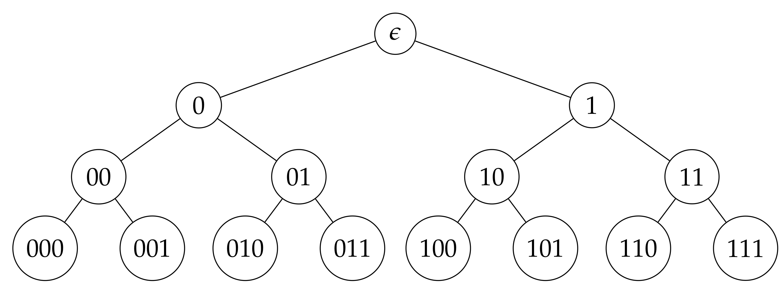
4.3. Around Perfect Binary Trees

Definition 4.
A rooted binary tree is called perfect if all its interior nodes have two children and all leaves have the same depth or same level.
A perfect binary tree is completely determined by the number of its leaves. To produce a perfect binary tree with levels we need to create 2 1 proofs.
A perfect binary tree M with 2 1 nodes as a poset consists of words of length < in an alphabet of two letters, say { 0 , 1 } ; and w w iff w begins with w. So the empty word ϵ corresponds to the greatest element, the root. Figure 10 illustrates the case of M 4 .
Each perfect binary tree M + 1 with + 1 levels as a poset is the disjoint sum of two copies of one level smaller trees with the greatest element added
M + 1 ( M M ) + { ϵ } .
The last identity together with (28) and (29) implies
O u ( M + 1 ) { } + ( O u ( M ) × O u ( M ) ) , O d ( M + 1 ) ( O d ( M ) × O d ( M ) ) + { M } ,
i.e., up-set in ether empty or consists of ϵ and any up-sets in left and right subtrees. Note that for two incomparable nodes x and y the corresponding subtrees are disjoint: { x } { y } = . So down-sets in a tree are forests, i.e., disjoint unions of subtrees.
Proposition 7.
The following sequences are described recursively.
1.
The number u = | O u ( M ) | of up-sets in the perfect binary tree M :
u 1 = 0 , u + 1 = u 2 + 1
This is the sequence A003095 in [32]: 0 , 1 , 2 , 5 , 26 , 677 , 458330 , .
2.
The number v = | O u ( M ) / Aut M | of the orbits of such up-sets:
v 0 = 1 , v + 1 = v + 1 2 + 1 .
This is the sequence A006894 in [32]: 1 , 2 , 4 , 11 , 67 , 2279 , .
Proposition 8.
Each compatible total ordering on M + 1 given by (32), according to (30) can be obtained as a shuffle of two orderings on M . So the number of compatible total orderings of a perfect binary tree satisfies the recurrent relations
| Ord ( M + 1 ) | = | Ord ( M ) | 2 2 2 2 1 1
and, hence, admits the explicit formula
| Ord ( M + 1 ) | = ( 2 1 ) ! / k = 1 ( 2 k 1 ) 2 k ,
which can be interpreted as the number of all permutations on nodes of the tree multiplied the probability that the random permutation of nodes is compatible order on tree. This is the sequence A056972 in [32]: 1 , 2 , 80 , 21964800 , 74836825861835980800000 , .
Proposition 9.
The symmetry group of a perfect binary tree can be described recursively as a wreath product i.e., a semidirect product:
Aut ( M + 1 ) S 2 ( Aut ( M ) × Aut ( M ) ) ,
where the symmetric group S 2 = { e , τ } acts from the right by permutation on factors Aut ( M ) . So
M S 2 S 2 ( ( S 2 ) × ( S 2 ) ) × S 2 ( ( S 2 ) × ( S 2 ) ) ,
where copies of S 2 are indexed by internal nodes of M , i.e., by words w { 0 , 1 } * of length < 1 . Denote τ w the transposition from the corresponding copy of S 2 , the ‘symmetry in w’. It swaps between left and right subtrees at w (i.e. ( w 0 v ) τ w = w 1 v and ( w 1 v ) τ w = w 0 v for v { 0 , 1 } * ) and leaves the rest immobile.
The symmetry group Aut M admits a presentation with all of the above symmetries τ w as generators and relations are:
  • τ w 2 = e ;
  • τ w τ w = τ w τ w whenever w and w are incomparable in M (in this case τ w and τ w lives in two different factors of a direct product in (33));
  • τ w v τ w = τ w τ ( w v ) τ w (this is the multiplication rule for semidirect product in (33)).
The presentation (33) of elements of Aut M means that in each position corresponding to the internal node labeled by a word w one can put either transposition τ or the neutral element e. So Aut M has 2 2 1 1 elements τ W which are in one-to-one correspondence with subsets W on internal nodes (where transpositions τ are located). For any compatible total ordering σ Ord ( W ) ,
τ W : = τ σ 1 ( | W | ) τ σ 1 ( | W | 1 ) τ σ 1 ( 1 ) .

4.4. Distributed Generation of Posets

First we consider models from Examples 11–13 which are generalizations of models from Examples 5–7. We switch from sets to posets.
Notation 8.
Given finite poset N, denote M ( N ) = N O u ( N ) M ( Min N ) the Cartesian product of sets of probabilities distributions on all nonempty anti-chains Min N .
Example 11.
Let N be a poset and μ = ( Pr Min ( N ) ) N O u ( N ) M ( N ) are fixed probability distributions. We consider a Markov chain, where states are up-sets in N. Non-zero elements of transition matrix are
p ( N , N ) = g Sur ( m , N N ) i = 1 m Pr Min ( N ) ( g ( i ) ) , N Min N N N ,
and existence of surjection m N N implies | N N | m .
In the case of uniform distributions non-zero elements of transition matrix are
p ( N , N ) = | N N | ! · m | N N | · | Min N | m .
If N is a discrete poset then Min N = N are arbitrary subsets and we obtain a Markov chain from Example 5.
For this Markov chain the empty set is the absorbing state and all trajectories are strictly decreasing by inclusion. The subject of our interest is the absorption time τ m N = τ μ m N , a random variable which is equal to the number of steps it takes m provers to create all the proofs in up-set N . Note that τ m N = k iff p N k 1 = 0 and p N k = 1 The random variable τ m N takes values in the interval [ ht ( N ) , | N | ] , i.e., p N n = 0 for n < ht ( N ) and p N n = 1 for n | N | . S,o one can express the expectation of the absorption time via elements of powers of the transition matrix:
E τ m N = k = | N | k ( p N k p N k 1 ) = | N | 1 k = | N | 1 p N k .
From the other hand we have a recurrent formula involving matrix elements of the top raw of p as coefficients:
E τ m N = 1 + M Min N p N N M E τ m N M .
Now we can extend Example 6 and Proposition 3 about stochastic equivalence of two models to the case of posets. To do this, we need to go from a uniform distribution of probabilities to an arbitrary one.
Example 12
(Non-Markovian model). Let a probability distribution Pr Ord ( N ) on the set of compatible total orderings Ord ( N ) be given. Then, for each up-set N O u ( N ) the probability distributions on Ord ( N ) and on Min N
Pr Ord ( N ) ( σ ) : = σ Ord ( N ) σ | N = σ Pr Ord ( N ) ( σ ) , Pr Min N ( a ) : = σ Ord ( N ) σ ( a ) = 1 Pr Ord ( N ) ( σ ) ,
are unique, turning the maps N σ σ | N N σ ( σ ) 1 ( 1 ) Min N into morphisms of probability spaces. (Here the restriction σ | N is defined by (31).) Then we can consider the Markov chain from the previous Example 11 with probability distributions on anti-chains Min N obtained by composing of (37)
Pr Min N ( a ) : = σ Ord ( N ) σ | N ( a ) = 1 Pr Ord ( N ) ( σ ) .
An element of Cartesian degree ( Ord N ) m corresponds to the choice of a ranging σ i Ord ( N ) by each prover 1 i m . It completely determines a trajectory for this Markov chain, i.e., strongly decreasing sequence of up-sets of not yet proven candidates
N = N 0 N 1 N 2 N k = , N j + 1 = N j σ i | N j 1 ( 1 ) | 1 i m ,
together with selection in each moment 0 j < k by each prover 1 i m the first possible proof-candidate σ i | N j 1 ( 1 ) Min N j according to its own ranging. Directly from the definition one can see that conditional probabilities of such selections are given by (38).
Consider the case when N is a discrete poset and, hence, Min N = N are arbitrary subsets. If we additionally suppose that the initial distribution Pr Ord N is uniform, then for each N the matched distributions Pr Ord N and Pr Min N are also uniform because the numbers of summands in (37) are independent on σ N and a Min N respectively. They are naturally indexed in the first case by | N | ! / | N | ! permutations of N preserving order between elements of N and in the second case by ( | N | 1 ) ! permutations preserving a. So, this covers the case of Example 6 and Proposition 3.
It should be emphasized that the construction in this example is less universal than the general case of Example 11. For instance in the case of N = { a } { b < c } from (38) we obtain Pr { a , b } ( a ) = Pr N ( a < b < c ) , Pr { a , c } ( a ) = Pr N ( a < b < c , b < a < c ) and the restriction Pr { a , b } ( a ) Pr { a , c } ( a ) . In particular, the probability distributions μ = ( Pr Min N ) N O u ( N ) minimizing E τ μ m N do not come from this example.
Example 13
(Factorization by the symmetry group). Consider the data from Example 11 in the case when all probability measures ( Pr Min N ) N O u ( N ) are Aut N -invariant, i.e.
Pr Min N σ = Pr Min N , σ Aut N .
By Proposition 2, the canonical projection π : O u ( N ) O d ( N ) / Aut O u ( N ) to the orbit set is a lumping map.
So we obtain a Markov chain with the set of states O u ( N ) / Aut N the transition probabilities between orbits are given by sums (6) applied to (34)
p ( [ N ] , [ N ] ) = N [ N ] p ( N , N ) = N [ N ] N Min N N N g : m N N i = 1 m Pr Min ( N ) ( g ( i ) )
  • In the case of discrete poset N, elements of O u ( N ) are all subsets of N, the symmetry group Aut N consists of all permutations and orbits O u ( N ) / Aut N are just integers 0 , 1 , , | N | identified with cardinalities of subsets. So we obtain a Markov chain from Example 7.
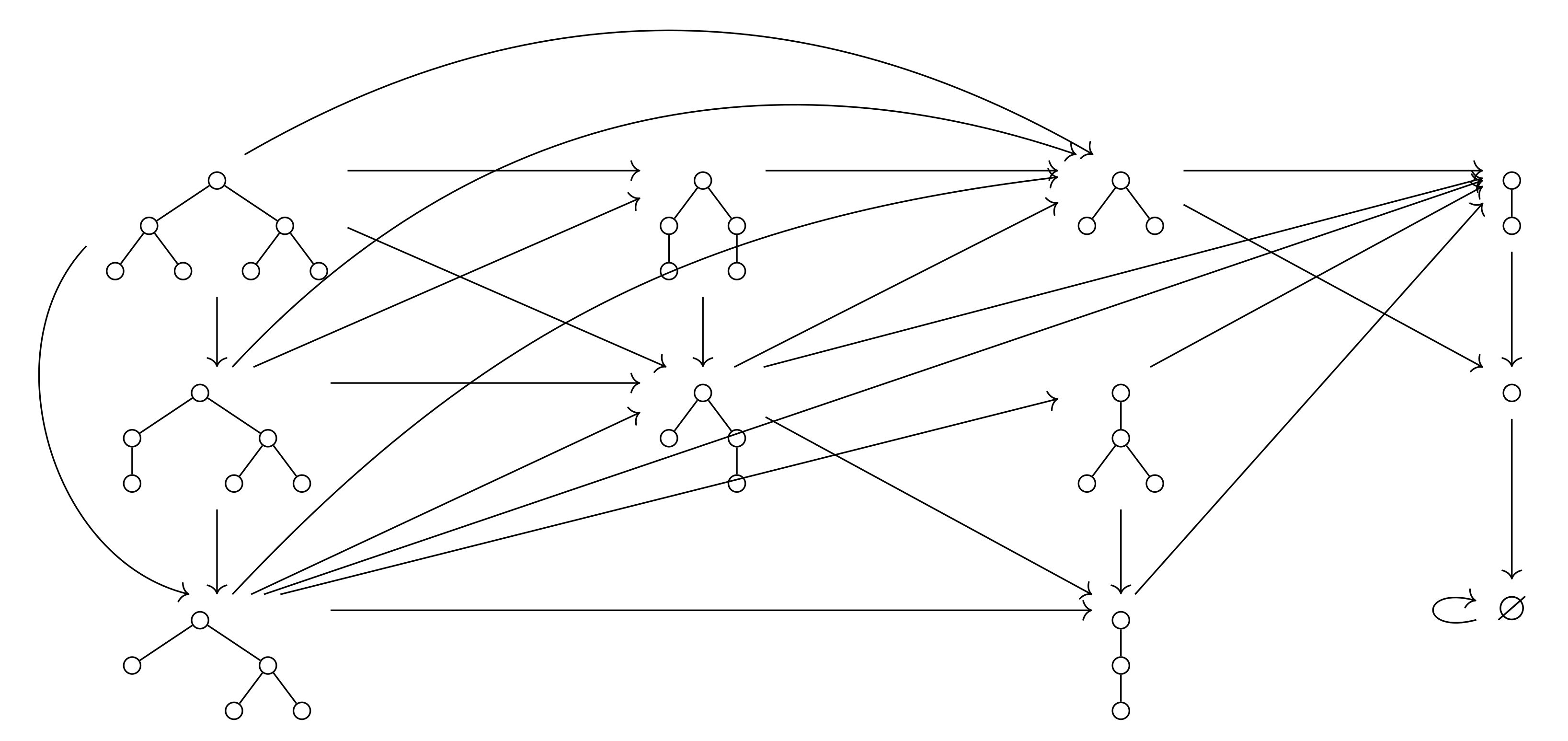
  • In the case N = M of perfect binary tree with levels the states of the Markov chain from Example 11 (resp. from Example 13) are up-sets in M (res. orbits of such up-sets under action of Aut M ). According to Proposition 7 the numbers of such up-sets N or orbits of up-sets grow rapidly depending on . Moreover, if we decide to consider not only uniform probability distributions on anti-chains Min N we obtain a lot of additional parameters.
    For the case = 3 , the oriented graph of the Markov chain from Example 13 for M 3 is presented on Figure 11. It has 11 states, has no cycles including loops (except of the loop for the final state ⌀); the transition matrix is triangular; Aut M 3 -invariant probability measures on different Min N depends totally on 3 parameters.

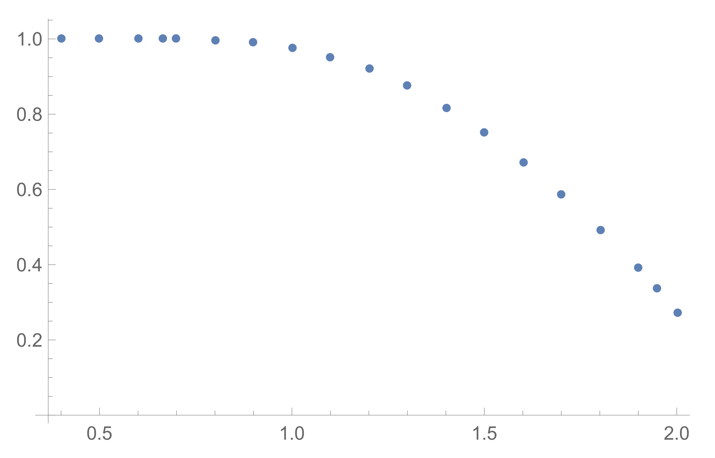
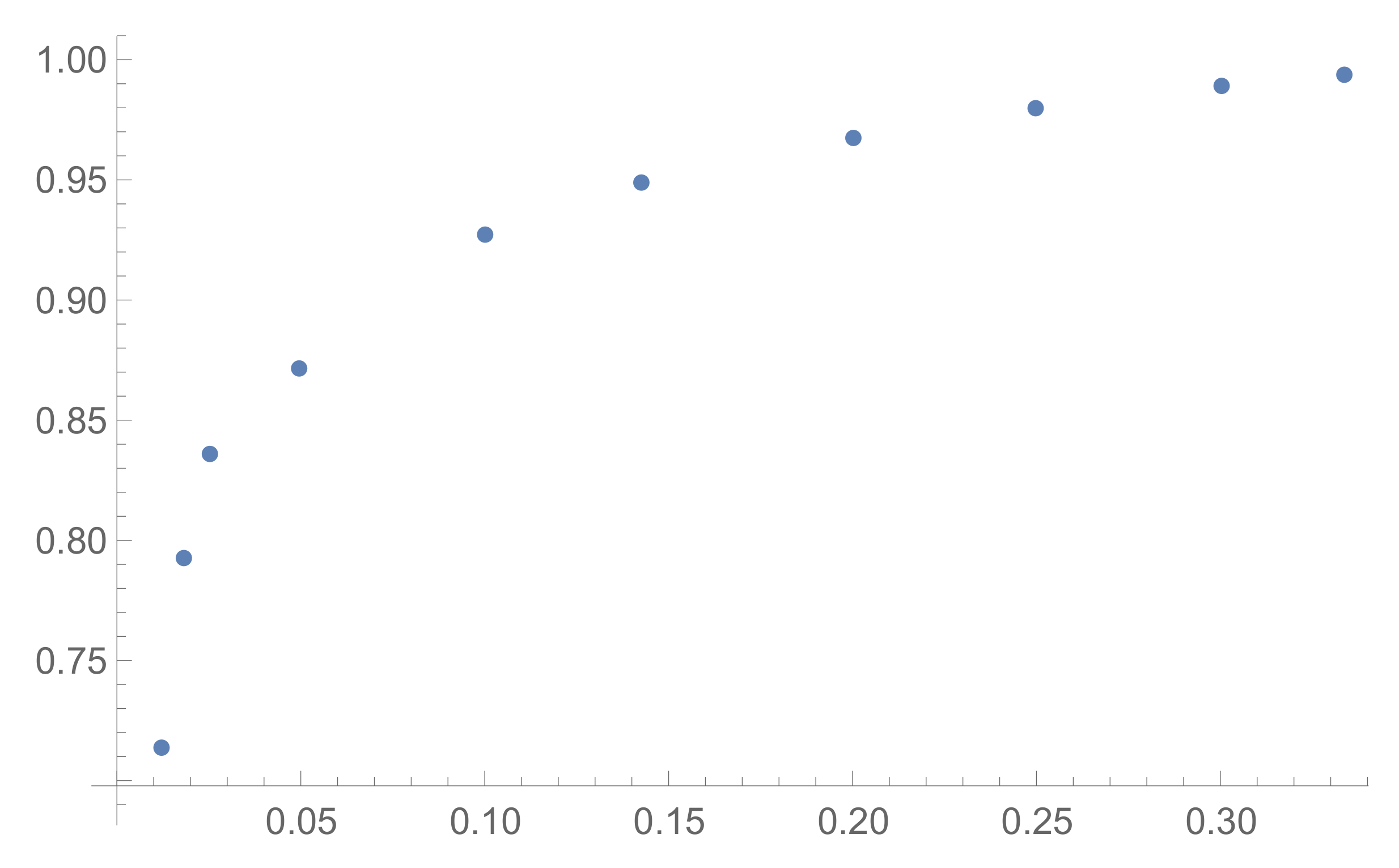
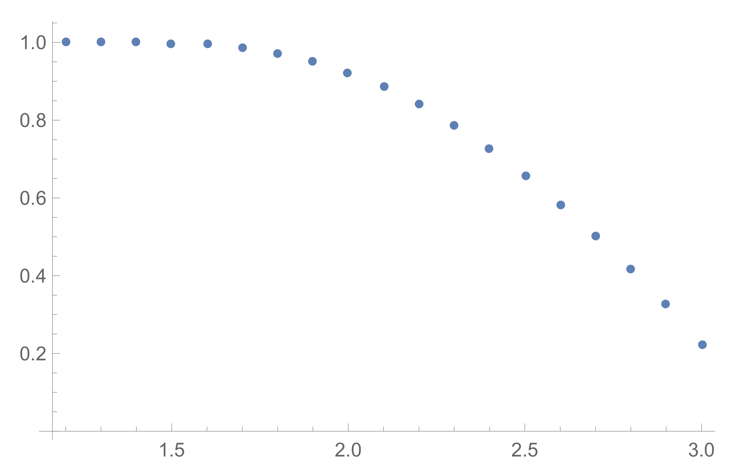
4.5. Some Asymptotics for τ m N

For fixed finite poset N and a fixed number of provers m 2 the subject of our interest is to find minimum of E τ μ m N over all possible ( Aut N -invariant) measures μ = ( Pr Min N ) N N , and their limits when m . We describe this asymptotic behavior in terms of heights of up-sets.
Next we show that expectation E τ m N tends to its minimal possible value (equal the height ht ( N ) ) when the number of provers m rise. Note that each finite poset N can represented as disjoint union
N = k = 0 ht ( N ) 1 Min N / k , N / 0 : = N , N / ( k + 1 ) = N / k Min N / k .
Proposition 10.
Let Pr Min N / k ( a ) > 0 for all integers k [ 0 , ht ( N ) 1 ] and for all a Min N k . Then
lim m E τ m N = ht ( N ) .
Proof. 
For each ε > 0 there exists m 0 N such that for all m m 0 for all k from [ 0 . . ht N ) all elements of Min N / k will be proved on ( k + 1 ) th step with probability > 1 ε . □
Some types of posets N we will obtain asymptotic in the form
min μ M ( N ) E τ μ m N m ht ( N ) + α N γ N m + o ( γ N m ) , 0 γ N < 1 .
The case is suitable when N admits a rich symmetry enough.
Proposition 11.
Let N be a finite poset such that in notations of (40) for each N / k , k = 0 , 1 , , ht N 1 its symmetry group Aut N / k acts transitive on Min N / k . In this case for large number of provers m accurate to o ( 1 1 / wd N ) m we have
min μ M ( N ) E τ μ m N m ht N + κ N · wd N · ( 1 1 / wd N ) m ,
where κ N is a number of such k that # Min N / k = wd N .
Proof. 
Transitivity of the action of Aut N / k on Min N / k implies that uniform probability distribution on Min N / k is optimal. Denote the right hand side of (42) by Φ ( N ) and n k = | Min N / k | . By induction, we can write min μ M ( N / k ) E τ μ m N / k as a sum
1 + n k ! m n k n k m min μ M ( N / ( k + 1 ) ) E τ μ m N / ( k + 1 ) + n k ( n k 1 ) ! m n k 1 n k m min μ M ( N / ( k + 1 ) + ) E τ μ m N / ( k + 1 ) + + ,
where N / ( k + 1 ) + is N / ( k + 1 ) with one additional element from Min N / k (in all cases we obtain isomorphic posets); and “⋯” means summands which are small with respect to ( 1 1 / wd N ) m . Next we remove small terms from inclusion-exclusion formula (5) for Striling numbers:
min μ M ( N / k ) E τ μ m N / k m 1 + 1 n k ( 1 1 / n k ) m Φ ( N / ( k + 1 ) ) + n k ( 1 1 / n k ) m · ht N / k + m Φ ( N / ( k + 1 ) ) + Φ ( Min N / k ) .
Then, in all three possible cases wd N / ( k + 1 ) = wd N / k , n k = wd N / k or wd N / ( k + 1 ) < wd N / k , n k = wd N / k or wd N / ( k + 1 ) = wd N / k , n k < wd N / k we have Φ ( N / ( k + 1 ) ) + Φ ( Min N / k ) Φ ( N / k ) accurate to o ( 1 1 / wd N ) m . □
The perfect binary tree M satisfies assumptions of Proposition 11; we have ht M = , wd M = 2 1 and κ M = 1 .
Corollary 2.
For perfect binary tree M and for a large number of provers m:
min μ M ( M ) E τ μ m M m + 2 1 2 1 1 2 1 m ,
and the corresponding probability
Pr ( τ m M = ) m 1 2 1 2 1 1 2 1 m .
Next we consider the case of coproducts of chains
N = 1 i k n i = { ( i , j ) | 1 i k 1 j n i } , n i > 0 .
A kth copower N = 1 i k n of a chain n satisfies assumptions of Proposition 11. We have ht N = κ N = n and wd N = k .
Corollary 3.
For positive integer k and n
min μ M ( 1 i k n ) E τ μ m 1 i k n m n + k n ( 1 1 / k ) m + o ( 1 1 / k ) m .
If assumptions of Proposition 11 about symmetry of poset N are violated, asymptotic formulas (41) become more complicated. We can obtain explicit formula for the simplest such case.
Proposition 12.
For positive integers n 1 , n 2 with accuracy o ( | n 2 n 1 | + 2 ) m
min μ M ( n 1 n 2 ) E τ μ m n 1 n 2 m n 1 n 2 + n 1 n 2 n 1 n 2 n 1 + n 2 + 1 | n 1 n 2 | + 1 1 1 | n 2 n 1 | + 2 m ,
where n 1 n 2 = max { n 1 , n 2 } and n 1 n 2 = min { n 1 , n 2 }
Proof. 
Firstly we show that if n 2 > n 1 > 0 , then numbers α n 1 n 2 + 1 satisfy Pascal recursive rule and boundary conditions
α n 1 n 2 + 1 = ( α ( n 1 1 ) ( n 2 1 ) + 1 ) + ( α n 1 ( n 2 1 ) + 1 ) ,
α 0 n = α n = 0 , α n n = 2 n .
(The second boundary condition comes from (46).)
Suppose that n 2 > n 1 and probability distribution Pr Min n 1 n 2 on Min n 1 n 2 = { ( 1 , 1 ) , ( 1 , 2 ) } is given by Pr Min n 1 n 2 ( 1 , j ) = p j , j = 1 , 2 and p 1 + p 2 = 1 . Then by induction E τ m n 1 n 2 can be written as
1 + p 1 m min E τ m n 1 1 n 2 + p 2 m min E τ m n 1 n 2 1 + ( 1 p 1 m p 2 m ) min E τ m n 1 1 n 2 1 .
Removing a priori small terms, one rewrite this expression as
n 2 + α n 1 1 n 2 1 1 n 2 n 1 + 2 m + p 1 m + α n 1 n 2 1 1 n 2 n 1 + 1 m p 2 m .
The method of Lagrange multipliers for m gets p 1 = 1 / ( n 2 n 1 + 2 ) and
min E τ m n 1 n 2 n 2 + ( 1 + α n 1 1 n 2 1 + α n 1 n 2 1 ) 1 n 2 n 1 + 2 m .
And so we obtain Pascal rule (47).
Next we find the generating function for the double sequence α n 1 n 2 + 1 :
f ( x , y ) = k = 0 n = k ( α k n + 1 ) x k y n k = 1 + x ( 1 x ) ( 1 x y ) .
This explicit expression can be obtained from simplification of ( 1 x y ) f ( x , y ) using recurrent relation (47) and boundary conditions (48).
Finally we extract coefficients α k n + 1 = [ x k y n k ] f ( x , y ) from
n = 0 k = 0 n ( α k n + 1 ) x k y n k = ( 1 + x ) ( 1 + x + x 2 + ) 1 + ( x + y ) + ( x + y ) 2 + .
The next step would be:
Problem 1.
Find asymptotic formula (41) for arbitrary finite coproduct (45) of finite chains.
For each fixed finite poset N one can consider its nth copowers i n N and then study the dependence of absorption time τ m i n N on the number of copies n and number of provers m. If N is a singleton we obtain a random variable τ m n from Example 7.
Hypothesis 7.
For finite poset N, there exists a generalization of function h ( x ) from Hypothesis 2, given by the limit
h N ( x ) : = lim m , n n / m x min E τ m i n N .
This function has a number of properties that generalize the properties of h ( x ) .

4.6. Practical Realization of Proof Trees Generation

For the stable and efficient functioning of the sidechain, it is necessary that the following conditions are met:
  • All transactions that the blockforger plans to include in the issued block must be processed within the time slot, i.e., the time allotted for the creation of this block, and the correspondent proof tree must be completely built;
  • The number of these transactions should be the maximum possible, for which the probability of constructing the corresponding proof tree is close to 1.
The first condition is necessary in order to minimize or reduce to zero the number of proofs that will be created but not used, i.e., so that the work of the provers is not done in vain. The second condition is necessary to maximize the sidechain throughput.
Therefore, it is necessary to define, given the network parameters (such as the length of the time slot and the number of active provers), such a maximum number of leaves so that the corresponding proof tree is completely built in a time slot with a probability of at least 1 ε for sufficiently small ε > 0 .
We assume that the time slot length is fixed throughout the life of the sidechain. We also assume that the time required to form one proof is the same throughout the lifetime of the sidechain for all miners. This time will be called a tick. The whole part of dividing the time slot duration by the tick duration is equal to the number of proofs that each active miner can build in one time slot. Since the lengths of the time slot and tick are fixed, the number of such proofs during the time slot is also fixed. However, the number of provers may vary.
The task is to determine the maximum number of transactions in a block for a given numbers k of ticks in a time slot, m of provers, for which the corresponding proof tree will be built with a probability of at least 1 ε .
To solve this problem, we will use the results of Section 3, and also make the following assumptions.
We will assume that provers build all levels of the proof tree sequentially, from leaves to root. First probabilities are calculated so that the corresponding level will be completely built in 1 , 2 , 3 , etc., ticks (for a given number of proofs and provers). Then, using these probabilities we find the number of levels that will be built with probability 1 ε in k tics:
Pr ( τ m M k ) k 1 + + k k k 1 , , k 1 1 r Pr ( τ m 2 r 1 = k r ) .
If Pr ( τ m 2 1 = 1 ) 1 , we can reduce the previous formula as
Pr ( τ m M k ) k + 1 + + k k k + 1 , , k 1 < r Pr ( τ m 2 r 1 = k r ) .
Table 1, which indicates the probabilities of constructing a given number of proofs for a given number of provers for a given number of ticks, is auxiliary for solving our problem.
Each row in Table 1 corresponds to a certain fixed number of provers. The columns correspond to the levels of the proof tree, starting from the second from the root. For example, in a cell with coordinates 512 provers, 32 proofs there is a list of two pairs of numbers: 1 ; 0 : 999997 2 ; 0.000003 . This means that 512 provers will build 32 proofs in exactly 1 tick with a probability of 0.999997 and in exactly 2 ticks with a probability of 0.000003 . Therefore, the probability of building 32 proofs in no more than 2 ticks is non-distinguished from 1.
Let us calculate the maximum number of transactions in a block that 512 provers can process with a probability of at least 0.95 in 9 ticks.
The first 5 levels (including the root) will be processed each in 1 tick with a probability almost equal to 1. Therefore, we have at most 4 ticks for building the remaining levels. Note that the eighth level can be built in 1 tick with a very small probability of 0.088899 , so this level requires two ticks. The probability of building it in no more than two ticks will be 0.088899 + 0.911101 , which is practically equal to 1. That is, if there are 8 levels in the tree, then 2 ticks remain for the 6th and 7th levels, 1 tick for each level. According to the results in Table 1, the probability of building these two levels in 2 ticks is 0.999997 · 0.980019 = 0.980016 , which is more than 0.95 , therefore, a block with 128 transactions will be released with a probability of at least 0.95 , which satisfies our requirements.
Similarly, it can be shown that the probability of a block with 256 transactions being released is significantly less than 0.95 . Therefore, if there are 512 active provers, it is recommended to issue a block with 128 transactions.
Based on Table 1, Table 2 was built, which shows the recommended number of transactions in a block for a different number of provers. All possible values of the number of provers are divided here into intervals, in accordance with the number of transactions in the block. For example, 2176 provers will build a block with 512 transactions with a probability of 0.95001 , and 2175 provers with a probability of 0.949825 . Therefore, if the number of provers is at least 2176, then the recommended number of transactions in a block is 512, and if the number of provers is from 998 to 2175, then the recommended number of transactions is 256.
Remark 6.
One can solve (44) as equation with respect to the number of provers:
m ln n ln ε ln ( 1 1 / n ) , n = 2 1 , ε = 1 Pr ( τ m M = ) .
In our case n = 256 and ε = 0.05 and we have m 2182 . This coincides with the last boundary 2176 in Table 2 with accuracy ( 2182 2176 ) / 2176 0.3 % .

5. Conclusions

This paper is a part of series of works concerning the sidechains with Latus consensus and zk-SNARKs. The previous works were [30], which may be considered as a restricted preimage of this one, and [46], which researches some game theoretical aspects, occurring when provers set prices for their proofs. All articles from the series are devoted to some concrete practical problems, which may be formulated, in general, as conditions of fully decentralized sidechains based on the Latus consensus protocol. We partially solved these problems analyzing existed mathematical models and methods and creating our specific ones, like probability distributions on partially ordered sets, which are the most suitable for existing purposes. The specific characteristics of this work is some numbers of hypothesis, which were formulated based on a large amount of numerical results obtained using infinite-precision calculations. For our opinion, the task to prove all them seems to be rather non-trivial. The numerical results, obtained at the end of the article, allows to chose correct values of some parameters to achieve stability and high throughput in sidechains. The further researches, which continue the series, are planned to be devoted to a more general, more efficient, and more complicated approach, when a series of blocks are built simultaneously, allowing provers to create proofs for several sequential blocks. Note that this approach allows one to increase essentially without losing stability in the sidechain, and it is therefore useful and interesting.

Author Contributions

Conceptualization, R.O.; Data curation, A.G.; Formal analysis, Y.B. and L.K.; Software, H.N. All authors have read and agreed to the published version of the manuscript.

Funding

This work was supported in part by the National Research Foundation of Ukraine under Grant 2020.01/0351.

Institutional Review Board Statement

Not applicable.

Informed Consent Statement

Not applicable.

Data Availability Statement

Not applicable.

Acknowledgments

We would like to thanks Ulrich Haboeck for the fruitful discussion and comments.

Conflicts of Interest

The authors declare that they have no conflict of interest.

Abbreviations

The following abbreviations are used in this manuscript:
zk-SNARKZero-Knowledge Succinct Non-Interactive Argument of Knowledge
SCSidechain
MCMainchain
PoWProof of work
PoSProof of stake
UTXOUnspent transaction output
iffif and only if
posetpartially ordered set
ppmparts per million

References

  1. Rootstock: Smart Contracts on Bitcoin Network. 2018. Available online: https://www.rsk.co/ (accessed on 10 October 2021).
  2. Back, A.; Corallo, M.; Dashjr, L.; Friedenbach, M.; Maxwell, G.; Miller, A.; Poelstra, A.; Timón, J.; Wuille, P. Enabling Blockchain Innovations with Pegged Sidechains. 2014. Available online: https://blockstream.com/sidechains.pdf (accessed on 10 October 2021).
  3. Kiayias, A.; Zindros, D. Proof-of-Work Sidechains. 2018. Available online: https://ia.cr/2018/1048 (accessed on 11 October 2021).
  4. Garoffolo, A.; Kaidalov, D.; Oliynykov, R. Zendoo: A zk-SNARK Verifiable Cross-Chain Transfer Protocol Enabling Decoupled and Decentralized Sidechains. arXiv 2020, arXiv:2002.01847. [Google Scholar]
  5. Pass, R.; Shi, E. FruitChains: A Fair Blockchain. Cryptology ePrint Archive, Report 2016/916. 2016. Available online: https://ia.cr/2016/916 (accessed on 11 October 2021).
  6. VeriBlock Inc. Proof-of-Proof and VeriBlock Blockchain Protocol Consensus Algorithm and Economic Incentivization Specifications. 2019. Available online: http://bit.ly/vbk-wp-pop (accessed on 12 October 2021).
  7. Gaži, P.; Kiayias, A.; Russell, A. Tight consistency bounds for bitcoin. In Proceedings of the 2020 ACM SIGSAC Conference on Compute and Communications Security, Virtual Event, 9–13 November 2020; pp. 819–838. [Google Scholar]
  8. Karpinski, M.; Kovalchuk, L.; Kochan, R.; Oliynykov, R.; Rodinko, M.; Wieclaw, L. Blockchain Technologies: Probability of Double-Spend Attack on a Proof-of-Stake Consensus. Sensors 2021, 21, 6408. [Google Scholar] [CrossRef] [PubMed]
  9. Kovalchuk, L.; Kaidalov, D.; Nastenko, A.; Rodinko, M.; Oliynykov, R. Probability of double spend attack for network with non-zero synchronization time. In Proceedings of the 21th Central European Conference on Cryptology (CECC 2021), Budapest, Hungary, 23–25 June 2021; pp. 52–54. [Google Scholar]
  10. Kovalchuk, L.; Kaidalov, D.; Nastenko, A.; Rodinko, M.; Shevtsov, O.; Oliynykov, R. Decreasing security threshold against double spend attack in networks with slow synchronization. Comput. Commun. 2020, 154, 75–81. [Google Scholar] [CrossRef]
  11. Garoffolo, A.; Viglione, R. Sidechains: Decoupled Consensus Between Chains. arXiv 2018, arXiv:1812.05441. [Google Scholar]
  12. Kiayias, A.; Russell, A.; David, B.; Oliynykov, R. Ouroboros: A provably secure proof-of-stake blockchain protocol. In CRYPTO 2017, Part I; Lecture Notes in Computer Science; Springer: Heidelberg, Germany, 2017; Volume 10401, pp. 357–388. [Google Scholar]
  13. Garay, J.; Kiayias, A.; Leonardos, N. The bitcoin backbone protocol: Analysis and applications. In Advances in Cryptology-EUROCRYPT 2015, Part II; Lecture Notes in Computer Science; Springer: Berlin/Heidelberg, Germany, 2015; Volume 9057, pp. 281–310. [Google Scholar]
  14. Ben-Sasson, E.; Chiesa, A.; Tromer, E.; Virza, M. Succinct Non-Interactive Zero Knowledge for a von Neumann Architecture. 2013. Available online: https://ia.cr/2013/879 (accessed on 10 October 2021).
  15. Bowe, S.; Gabizon, A. Making Groth’s zk-SNARK Simulation Extractable in the Random Oracle Model. 2018. Available online: https://ia.cr/2018/187 (accessed on 10 October 2021).
  16. Reitwiessner, C. zkSNARKs in a Nutshell. 2016. Available online: https://blog.ethereum.org/2016/12/05/zksnarks-in-a-nutshell/ (accessed on 17 October 2021).
  17. Goldwasser, S.; Micali, S.; Rackoff, C. The knowledge complexity of interactive proofs. SIAM J. Comput. 1989, 18, 186–208. [Google Scholar] [CrossRef]
  18. Bitansky, N.; Canetti, R.; Chiesa, A.; Tromer, E. From Extractable Collision Resistance to Succinct Non-Interactive Arguments of Knowledge, and Back Again. Cryptology ePrint Archive, Report 2011/443. 2011. Available online: https://ia.cr/2011/443 (accessed on 10 October 2021).
  19. Groth, J. Short pairing-based non-interactive zero-knowledge arguments. In ASIACRYPT 2010; Abe, M., Ed.; Lecture Notes in Computer Science; Springer: Berlin/Heidelberg, Germany, 2010; Volume 6477, pp. 321–340. [Google Scholar]
  20. Gennaro, R.; Gentry, C.; Parno, B.; Raykova, M. Quadratic Span Programs and Succinct NIZKs without PCPs. Cryptology ePrint Archive, Report 2012/215. 2012. Available online: https://ia.cr/2012/215 (accessed on 12 October 2021).
  21. Parno, B.; Gentry, C.; Howell, J.; Raykova, M. Pinocchio: Nearly Practical Verifiable Computation. Cryptology ePrint Archive, Report 2013/279. 2013. Available online: https://ia.cr/2013/279 (accessed on 12 October 2021).
  22. Groth, J. On the Size of Pairing-Based Non-interactive Arguments. In Advances in Cryptology–EUROCRYPT 2016; Fischlin, M., Coron, J.S., Eds.; Lecture Notes in Computer Science; Springer: Berlin/Heidelberg, Germany, 2016; Volume 9666, pp. 305–326. [Google Scholar]
  23. Hopwood, D.; Bowe, S.; Hornby, T.; Wilcox, N. Zcash Protocol Specification: Version 2021.2.16 [NU5 Proposal]. 2021. Available online: https://zips.z.cash/protocol/protocol.pdf (accessed on 12 October 2021).
  24. Mina. Started by O(1) Labs. 2021. Available online: https://minaprotocol.com (accessed on 17 October 2021).
  25. Grassi, L.; Khovratovich, D.; Rechberger, C.; Roy, A.; Schofnegger, M. Poseidon: New Hash Functions for Zero Knowledge Proof Systems. Cryptology ePrint Archive, Report 2019/458. 2019. Available online: https://ia.cr/2019/458 (accessed on 12 October 2021).
  26. Kovalchuk, L.; Oliynykov, R.; Rodinko, M. Security of the Poseidon Hash Function Against Non-Binary Differential and Linear Attacks. Cybern Syst. Anal. 2021, 57, 268–278. [Google Scholar] [CrossRef]
  27. Haböck, U.; Garoffolo, A.; Benedetto, D.D. Darlin: Recursive Proofs using Marlin. Cryptology ePrint Archive, Report 2021/930. 2021. Available online: https://ia.cr/2021/930 (accessed on 12 October 2021).
  28. Chiesa, A.; Hu, Y.; Maller, M.; Mishra, P.; Vesely, N.; Ward, N. Marlin: Preprocessing zkSNARKs with Universal and Updatable SRS. In Proceedings of the Advances in Cryptology-EUROCRYPT 2020-39th Annual International Conference on the Theory and Applications of Cryptographic Techniques, Part I, Zagreb, Croatia, 10–14 May 2020; Canteaut, A., Ishai, Y., Eds.; Lecture Notes in Computer Science. Springer: Berlin/Heidelberg, Germany, 2020; Volume 12105, pp. 738–768. [Google Scholar]
  29. Boneh, D.; Drake, J.; Fisch, B.; Gabizon, A. Halo Infinite: Recursive zk-SNARKs from Any Additive Polynomial Commitment Scheme. Cryptology ePrint Archive, Report 2020/1536. 2020. Available online: https://ia.cr/2020/1536 (accessed on 12 October 2021).
  30. Bespalov, Y.; Garoffolo, A.; Kovalchuk, L.; Nelasa, H.; Oliynykov, R. Models of distributed proof generation for zk-SNARK-based blockchains. In Theoretical and Applied Cryptography; Belarusian State University: Minsk, Belarus, 2020; pp. 112–120. [Google Scholar]
  31. Stanley, R.P. Enumerative Combinatorics, 2nd ed.; Cambridge Studies in Advanced Mathematics, 49; Cambridge University Press: Cambridge, UK, 2011; Volume 1. [Google Scholar]
  32. The OEIS Foundation Inc. The On-Line Encyclopedia of Integer Sequences. Available online: https://oeis.org (accessed on 17 October 2021).
  33. Kemeny, J.G.; Snell, J.L. Finite Markov Chains; Undergraduate Texts in Mathematics; Springer: Berlin/Heidelberg, Germany, 1976. [Google Scholar]
  34. Ben-Israel, A.; Greville, T.N. Generalized Inverses: Theory and Applications, 2nd ed.; CMS Books in Mathematics; Springer: Berlin/Heidelberg, Germany, 2003. [Google Scholar]
  35. D’Angeli, D.; Donno, A. Crested products of Markov chains. Ann. Appl. Probab. 2009, 19, 414–453. [Google Scholar] [CrossRef]
  36. Levin, D.A.; Peres, Y.; Wilmer, E.L. Markov Chains and Mixing Times, 2nd ed.; AMS: Providence, RI, USA, 2017. [Google Scholar]
  37. O’Neill, B. The Classical Occupancy Distribution: Computation and Approximation. Am. Stat. 2021, 75, 364–375. [Google Scholar] [CrossRef]
  38. Jiang, Z. An Upper Bound on Stirling Number of the Second Kind. 2015. Available online: https://blog.zilin.one/2015/02/25/an-upper-bound-on-stirling-number-of-the-second-kind/ (accessed on 12 October 2021).
  39. Corless, R.; Gonnet, G.; Hare, D.; Jeffrey, D.; Knuth, D. On the Lambert W function. Adv. Comput. Math. 1996, 5, 329–359. [Google Scholar] [CrossRef]
  40. Moser, L.; Wyman, M. Stirling numbers of the second kind. Duke Math. J. 1958, 25, 29–48. [Google Scholar] [CrossRef]
  41. Bender, E.A. Central and local limit theorems applied to asymptotic enumeration. J. Combin. Theory Ser. A 1973, 15, 91–111. [Google Scholar] [CrossRef] [Green Version]
  42. Temme, N.M. Asymptotic estimates of Stirling numbers. Stud. Appl. Math. 1993, 89, 233–243. [Google Scholar] [CrossRef] [Green Version]
  43. Roman, S. Lattices and Ordered Sets; Springer: Berlin/Heidelberg, Germany, 2008. [Google Scholar]
  44. Bespalov, Y. Categories: Between Cubes and Globes. Sketch I. Ukr. J. Phys. 2019, 64, 1125–1128. [Google Scholar] [CrossRef]
  45. Sidenko, S. Kac’s Random Walk and Coupon Collector’s Process on Posets. Ph.D. Thesis, MIT, Cambridge, MA, USA, 2008. [Google Scholar]
  46. Bespalov, Y.; Garoffolo, A.; Kovalchuk, L.; Nelasa, H.; Oliynykov, R. Game-Theoretic View on Decentralized Proof Generation in zk-SNARK Based Sidechains. In Proceedings of the Cybersecurity Providing in Information and Telecommunication Systems (CPITS 2021), CEUR Workshop Proceedings 2021, Online, 7–8 January 2021; Volume 2923, pp. 47–59. [Google Scholar]
Figure 1. α ( n / m ) .
Mathematics 09 03016 g001
Figure 2. γ ( n / m ) .
Mathematics 09 03016 g002
Figure 3. Graph of the function n 750 E τ 750 n as an approximation for h ( x ) .
Mathematics 09 03016 g003
Figure 4. Graph of the function n 50 E τ 50 n n 50 1 2 ln ( n 50 ) as an approximation for h ( x ) x 1 2 ln ( x ) .
Mathematics 09 03016 g004
Figure 5. λ 2 ( n / m ) .
Mathematics 09 03016 g005
Figure 6. γ 2 ( n / m ) .
Mathematics 09 03016 g006
Figure 7. γ 3 ( n / m ) .
Mathematics 09 03016 g007
Figure 8. λ 3 ( n / m ) .
Mathematics 09 03016 g008
Figure 9. γ 3 ( n / m ) .
Mathematics 09 03016 g009
Figure 10. Labeling of nodes for the perfect binary tree M 4 .
Mathematics 09 03016 g010
Figure 11. Markov chain for M 3 generation (factorized by Aut M 3 ).
Mathematics 09 03016 g011
Table 1. Probability distributions for τ m n accurate to ppm ( 10 6 ) and probabilities of tree creation for 9 tics.
m\n2481632641282569 tics
31;0.750000
2;0.250000
2;0.810764
3;0.187500
4;0.001736
3;0.346759
4;0.598575
5;0.054020
6;0.000643
7;0.000003
= 4
0.948934
41;0.875000
2;0.125000
1;0.093750
2;0.856554
3;0.049624
2;0.038452
3;0.791998
4;0.167602
5;0.001946
6;0.000002
= 4
0.998582
91;0.996094
2;0.003906
1;0.711365
2;0.288588
3;0.000047
1;0.010815
2;0.928031
3;0.061145
4;0.000009
2;0.006789
3;0.824258
4;0.168743
5;0.000210
= 5
0.892535
101;0.998047
2;0.001953
1;0.780602
2;0.219387
3;0.000011
1;0.028163
2;0.944047
3;0.027789
4;0.000001
2;0.036465
3;0.901558
4;0.061960
5;0.000017
= 5
0.951990
161;0.999969
2;0.000031
1;0.960000
2;0.040000
1;0.306798
2;0.693034
3;0.000168
1;0.000001
2;0.720767
3;0.279205
4;0.000027
3;0.323989
4;0.673970
5;0.002041
321;1.0000001;0.999598
2;0.000402
1;0.891278
2;0.108722
1;0.073443
2;0.926430
3;0.000127
2;0.490645
3;0.509350
4;0.000005
= 6
0.948374
331;1.0000001;0.999699
2;0.000301
1;0.904520
2;0.095480
1;0.089692
2;0.910235
3;0.000073
2;0.561396
3;0.438602
4;0.000002
= 6
0.961682
641;1.0000001;1.0000001;0.998446
2;0.001554
1;0.765182
2;0.234818
1;0.004182
2;0.995734
3;0.000084
2;0.226404
3;0.773595
4;0.000001
941;1.0000001;1.0000001;0.999972
2;0.000028
1;0.963319
2;0.036681
1;0.163487
2;0.836513
2;0.969308
3;0.030692
= 7
0.944377
951;1.0000001;1.0000001;0.999975
2;0.000025
1;0.965585
2;0.034415
1;0.173944
2;0.826056
2;0.973714
3;0.026286
= 7
0.950428
1281;1.0000001;1.0000001;1.0000001;0.995870
2;0.004130
1;0.562887
2;0.437113
1;0.000013
2;0.999930
3;0.000057
2;0.048095
3;0.951905
2561;1.0000001;1.0000001;1.0000001;0.999999
2;0.000001
1;0.990585
2;0.009415
1;0.304309
2;0.695691
2;0.999956
3;0.000044
4511;1.0000001;1.0000001;1.0000001;1.0000001;0.999981
2;0.000019
1;0.948528
2;0.051472
1;0.018313
2;0.981687
= 8
0.949452
4521;1.0000001;1.0000001;1.0000001;1.0000001;0.999981
2;0.000019
1;0.949314
2;0.050686
1;0.018930
2;0.981070
= 8
0.950256
5121;1.0000001;1.0000001;1.0000001;1.0000001;0.999997
2;0.000003
1;0.980019
2;0.019981
1;0.088899
2;0.911101
10241;1.0000001;1.0000001;1.0000001;1.0000001;1.0000001;0.999994
2;0.000006
1;0.959185
2;0.040815
21751;1.0000001;1.0000001;1.0000001;1.0000001;1.0000001;1.0000001;0.999995
2;0.000005
1;0.949825
2;0.050175
= 9
0.949820
21761;1.0000001;1.0000001;1.0000001;1.0000001;1.0000001;1.0000001;0.999995
2;0.000005
1;0.950016
2;0.049984
= 9
0.950011
Table 2. Recommended number of transactions in a block 2 1 , corresponding to the probability of block creation 1 ε = 0.95 (for a different numbers of provers).
m[1..3][4..9][10..32][33..94][95..451][452..2175]⩾2176
2 1 48163264128256
Publisher’s Note: MDPI stays neutral with regard to jurisdictional claims in published maps and institutional affiliations.

