Asymptotic Properties of One Mathematical Model in Food Engineering under Stochastic Perturbations

Abstract

For the example of one nonlinear mathematical model in food engineering with several equilibria and stochastic perturbations, a simple criterion for determining a stable or unstable equilibrium is reported. The obtained analytical results are illustrated by detailed numerical simulations of solutions of the considered Ito stochastic differential equations. The proposed criterion can be used for a wide class of nonlinear mathematical models in different applications.

1. Introduction

The aim of this paper is to show a simple criterion to determine a stable or unstable equilibrium for nonlinear systems with several equilibria under stochastic perturbations.

Different types of food models are popular in food engineering research (see, for instance, [1,2,3,4,5,6,7,8,9,10] and the references therein). To demonstrate the proposed criterion, the following mathematical model from the food engineering that is described by a nonlinear system with fractional nonlinearity [5]

$$\begin{array}{c}\frac{dA\left(t\right)}{dt}=r_{1}A\left(t\right)(1-kA\left(t\right))-\frac{\mu A\left(t\right)P\left(t\right)}{\beta +P\left(t\right)},\\ \frac{dP\left(t\right)}{dt}=r_{2}P\left(t\right)-\alpha A\left(t\right)P\left(t\right),t\ge 0,\end{array}$$

(1)

and the positive initial conditions $A\left(0\right)>0$ and $P\left(0\right)>0$ was chosen. Here, $A\left(t\right)$ and $P\left(t\right)$ are the concentration of aflatoxins and probiotics in a given food matrix, respectively. All parameters are positive constants and mean the following: $r_1$ is the intrinsic production rate of aflatoxins, $1/k$ is hte concentration of aflatoxins that can be formed within food matrix, $\mu$ is the detoxification ability of probiotics, $\beta$ is the half-saturation for the association term, $r_2$ is the rate of the occurrence/application of probiotics, and $\alpha$ is the rate of formation of aflatoxin–probiotics complexes.

Below, all non-negative equilibria of model (1) are considered and the property of stability or instability of each from these equilibria under stochastic perturbations is investigated. The obtained results refine and generalize the results of [5], where model (1) is investigated from the point of view of improving food systems and in the deterministic case only.

The proposed criterion can be used for a wide class of nonlinear mathematical models in different applications.

The remainder of the paper is organized as follows: In Section 2, three possible equilibria of model (1) are described with the necessary and sufficient conditions for the existence of the third equilibrium. In Section 3, a method of stochastic perturbations of model (1) is presented, and the linearization of the considered system of Ito’s stochastic differential equations for each from the possible equilibria of model (1) is obtained; in Section 4, some necessary auxiliary definitions and statements from the theory of stability of Ito’s stochastic differential equations are included, sufficient conditions of stability or instability for each from three possible equilibria are obtained, and a detail numerical analysis of model (1) under stochastic perturbations is presented via numerical simulations of its solutions. In Section 5, the conclusions are presented, and in Appendix A the standard method used in the paper for the linearization of a nonlinear system is shown.

2. Equilibria

The equilibria of the system (1) are defined by the conditions $A\left(t\right)=A=const$ and $P\left(t\right)=P=const$, i.e., by the system of two algebraic equations

$$\begin{array}{c}\left(r_1(1-kA)-\frac{\mu P}{\beta +P}\right)A=0,\hfill \\ \hfill (r_2-\alpha A)P=0,\end{array}$$

(2)

which has the following three solutions:

$$\begin{array}{ccc}{E}_0=(0,0),& E_1=\left(\frac{1}{k},0\right),& E_2=\left(\frac{r_2}{\alpha }, and\frac{\beta (\alpha -k{r}_2)}{k{r}_2-\alpha (1-\mu r_1^{-1})}\right).\end{array}$$

(3)

Note that the equilibria $E_0$ and $E_1$ always exist and, from (3), it follows that the positive equilibrium $E_2$ exists if and only if

$$\alpha >k{r}_2>\alpha \left(1-\frac{\mu }{r_1}\right).$$

(4)

Remark 1.

Note that in [5], one of the conditions for the existence of equilibrium $E_2$ is considered in the form $\alpha <k{r}_2$ and $r_{1}k{r}_2+\mu \alpha <r_1\alpha$, which is equivalent to $\alpha <k{r}_2<\alpha \left(1-{\displaystyle \frac{\mu }{r_1}}\right)$, which is evidently impossible.

3. Stochastic Perturbations and Linearization

Let $E^{*}=(A^{*},P^{*})$ be one from the equilibria (3) of system (1). Let us suppose that the system (1) is exposed to stochastic perturbations that are of the white noise type and are proportional to the deviation in the system state $\left(A\right(t),P(t\left)\right)$ from the equilibrium $E^{*}=(A^{*},P^{*})$. Then, the system (1) transforms to the following system of Ito’s stochastic differential equations [11]:

$$\begin{array}{c}dA\left(t\right)=\left(r_{1}A\left(t\right)(1-kA\left(t\right))-\frac{\mu A\left(t\right)P\left(t\right)}{\beta +P\left(t\right)}\right)dt+{\sigma }_1(A\left(t\right)-A^{*})d{w}_1\left(t\right),\hfill \\ dP\left(t\right)=(r_{2}P\left(t\right)-\alpha A\left(t\right)P\left(t\right))dt+{\sigma }_2(P\left(t\right)-P^{*})d{w}_2\left(t\right),\hfill \end{array}$$

(5)

where ${\sigma }_1$ and ${\sigma }_2$ are constants and $w_1\left(t\right)$ and $w_2\left(t\right)$ are the mutually independent standard Wiener processes.

Note that the equilibrium $E^{*}=(A^{*},P^{*})$ of initial system (1) is the solution of the stochastic system (5) too.

Calculating the Jacobian matrix for the system (5), we obtain the linear approximation (see (A3) in the Appendix A) of the nonlinear system (5) in the form

$$\begin{array}{c}d{z}_1\left(t\right)=\left(\left(r_1(1-2k{A}^{*})-\frac{\mu P^{*}}{\beta +P^{*}}\right)z_1\left(t\right)-\frac{\mu \beta A^{*}}{{(\beta +P^{*})}^2}{z}_2\left(t\right)\right)dt+{\sigma }_1{z}_1\left(t\right)d{w}_1\left(t\right),\hfill \\ d{z}_2\left(t\right)=(-\alpha P^{*}{z}_1\left(t\right)+(r_2-\alpha A^{*})z_2\left(t\right))dt+{\sigma }_2{z}_2\left(t\right)d{w}_2\left(t\right).\hfill \end{array}$$

(6)

Using (2). rewrite the linear system (6) separately for each equilibrium (3):

-

for $E_0$, the system (6) splits into two separate unrelated equations:

$$\begin{array}{c}d{z}_1\left(t\right)=r_1{z}_1\left(t\right)dt+{\sigma }_1{z}_1\left(t\right)d{w}_1\left(t\right),\\ d{z}_2\left(t\right)=r_2{z}_2\left(t\right)dt+{\sigma }_2{z}_2\left(t\right)d{w}_2\left(t\right);\end{array}$$

(7)

-

for $E_1$,

$$\begin{array}{c}d{z}_1\left(t\right)=\left(-r_1{z}_1\left(t\right)-\frac{\mu }{k\beta }{z}_2\left(t\right)\right)dt+{\sigma }_1{z}_1\left(t\right)d{w}_1\left(t\right),\hfill \\ d{z}_2\left(t\right)=-\left(\frac{\alpha }{k}-r_2\right)z_2\left(t\right)dt+{\sigma }_2{z}_2\left(t\right)d{w}_2\left(t\right);\hfill \end{array}$$

(8)

-

for $E_2$,

$$\begin{array}{c}d{z}_1\left(t\right)=\left(-\frac{k{r}_1{r}_2}{\alpha }{z}_1\left(t\right)-\frac{r_1^2{r}_2{(k{r}_2-\alpha (1-\mu r_1^{-1}))}^2}{{\alpha }^3\beta \mu }{z}_2\left(t\right)\right)dt+{\sigma }_1{z}_1\left(t\right)d{w}_1\left(t\right);\hfill \\ d{z}_2\left(t\right)=-\frac{r_1\alpha \beta (\alpha -k{r}_2)}{k{r}_2-\alpha (1-\mu r_1^{-1})}{z}_1\left(t\right)dt+{\sigma }_2{z}_2\left(t\right)d{w}_2\left(t\right).\hfill \end{array}$$

(9)

4. Stability

Let $\{\Omega ,\mathcal{F},\mathbf{P}\}$ be a complete probability space; $\{{\mathcal{F}}_t,t\ge 0\}$ be a nondecreasing family of sub-$\sigma$-algebras of $\mathcal{F}$, i.e., ${\mathcal{F}}_{t_1}\subset {\mathcal{F}}_{t_2}$ for $t_1<t_2$; and $\mathbf{E}$ be the mathematical expectation with respect to the measure $\mathbf{P}$.

Consider the system of two linear stochastic differential equations [12]

$$\begin{array}{c}{\dot{x}}_1\left(t\right)=a_{11}{x}_1\left(t\right)+a_{12}{x}_2\left(t\right)+{\sigma }_1{x}_1\left(t\right){\dot{w}}_1\left(t\right),\hfill \\ {\dot{x}}_2\left(t\right)=a_{21}{x}_1\left(t\right)+a_{22}{x}_2\left(t\right)+{\sigma }_2{x}_2\left(t\right){\dot{w}}_2\left(t\right),\hfill \end{array}$$

(10)

where $a_{ij}$ and ${\sigma }_i$, $i,j=1,2$ are constants; and $w_1\left(t\right)$ and $w_2\left(t\right)$ are the mutually independent standard Wiener processes.

Definition 1.

The zero solution of the system (6) is called stable in probability if for any ${\epsilon }_1>0$ and ${\epsilon }_2>0$, there exists $\delta >0$ such that the solution $z\left(t\right)=(z_1\left(t\right),z_2\left(t\right))$ of the system (6) satisfies the condition $\mathbf{P}\{{sup}_{t\ge 0}\left|z\left(t\right)\right|>{\epsilon }_1\}<{\epsilon }_2$, provided that $\mathbf{P}\left\{\right|z\left(0\right)|<\delta \}=1$.

Definition 2.

The zero solution of the system (10) is called:

-

mean square stable if for each $\epsilon >0$, there exists a $\delta >0$ such that ${\mathbf{E}\left|x\left(t\right)\right|}^2<\epsilon$, $x\left(t\right)=(x_1\left(t\right),x_2\left(t\right))$, and $t\ge 0$, provided that ${\left|x\left(0\right)\right|}^2<\delta$;

-

asymptotically mean square stable if it is mean square stable and, for each initial value $x\left(0\right)$, the solution $x\left(t\right)$ of the system (10) satisfies the condition $\underset{t\to \infty }{lim}\mathbf{E}{\left|x\left(t\right)\right|}^2=0$.

Remark 2.

Note that the level of nonlinearity of the system (5) is higher than one. It is known [12] that, in this case, a sufficient condition for asymptotic mean square stability of the zero solution of the linear approximation (6) at the same time is a sufficient condition for stability in probability of the appropriate equilibrium of the system (5). Therefore, to obtain the conditions for stability in probability of each from equilibria (3), it is enough to obtain the conditions for asymptotic mean square stability of the zero solution for each from the linear systems (7)–(9). On the other hand, the instability of one of the linear systems (7), (8), or (9) means the instability of the corresponding equilibrium of the system (5).

Remark 3.

In the deterministic case (${\sigma }_1={\sigma }_2=0$), the zero solution of the system (10) is asymptotically stable if and only if [12]

$$\begin{array}{c}Tr\left(A\right)=a_{11}+a_{22}<0,\\ det\left(A\right)=a_{11}{a}_{22}-a_{12}{a}_{21}>0.\end{array}$$

(11)

Lemma 1

([12]). Put $A=\parallel a_{ij}\parallel$, $i,j=1,2$, ${\delta }_i=\frac{1}{2}{\sigma }_i^2$, $i=1,2$. Suppose that the conditions (11) hold, $a_{12}\ne 0$, and

$$\begin{array}{cc}{\delta }_1<\frac{\left|Tr\right(A\left)\right|det\left(A\right)}{A_2},& {\delta }_2<\frac{\left|Tr\left(A\right)\right|det\left(A\right)-A_2{\delta }_1}{A_1-\left|Tr\left(A\right)\right|{\delta }_1},\\ A_1=det\left(A\right)+a_{11}^2,& A_2=det\left(A\right)+a_{22}^2.\end{array}$$

(12)

Then, the zero solution of the system (10) is asymptotically mean square stable.

Remark 4.

The proof of Lemma 1 is based on using the Lyapunov function $v=x^{\prime }Px$, where $P>0$ is the positive definite solution of the matrix equation $PA+A^{\prime }P=-Q$, $Q>0$, and estimating the negative definite square form $Lv<0$, where L is the generator [11] of the system (10). (For more details, see [12], p. 48.)

Corollary 1.

If $a_{12}{a}_{21}=0$, then the conditions (11) and (12) take the form

$$\begin{array}{cc}{a}_{11}<0,& a_{22}<0.\\ {\delta }_1<-a_{11},& {\delta }_2<-a_{22}.\end{array}$$

(13)

If $a_{22}=0$, then the conditions (11) take the form

$$a_{11}<0,a_{12}{a}_{21}<0.$$

(14)

4.1. Equilibrium $E_0$

From (11), it follows that in the deterministic case (${\sigma }_1={\sigma }_2=0$), the zero solution of the system (7) is unstable. However, under the conditions

$${\sigma }_1^2>2r_1,{\sigma }_2^2>2r_2,$$

(15)

the so-called “stabilization by noise” occurs [13,14].

In Figure 1, 25 trajectories of the solution of Equation (5) are shown with $r_1=0.1$, $r_2=0.15$, $\mu =0.1$, $k=2.5$, $\alpha =0.9$, $\beta =0.1$, $A\left(0\right)=0.15$, $P\left(0\right)=0.2$, ${\sigma }_1=0.18$, and ${\sigma }_2=0.19$. The equilibrium $E_0(0,0)$ is unstable, so the trajectories fill the whole space.

Figure 1. The 25 trajectories of $A\left(t\right)$ (blue) and $P\left(t\right)$ (green) of a solution of the system (5), with $r_1=0.1$, $r_2=0.15$, $\mu =0.1$, $k=2.5$, $\alpha =0.9$, $\beta =0.1$, $A\left(0\right)=0.15$, $P\left(0\right)=0.2$, ${\sigma }_1=0.18$, and ${\sigma }_2=0.19$.

In Figure 2, 25 trajectories of the solution of Equation (5) are shown with $A\left(0\right)=0.4$, $P\left(0\right)=0.6$, ${\sigma }_1=1.1$, and ${\sigma }_2=1.2$, and the same values of all other parameters as in Figure 1. The conditions (15) hold, stabilization by noise’ occurs, and all trajectories converge to the unstable equilibrium $E_0(0,0)$.

Figure 2. The 25 trajectories $A\left(t\right)$ (blue) and $P\left(t\right)$ (green) of a solution of the system (5), with $r_1=0.1$, $r_2=0.15$, $\mu =0.1$, $k=2.5$, $\alpha =0.9$, $\beta =0.1$, $A\left(0\right)=0.4$, $P\left(0\right)=0.6$, ${\sigma }_1=1.1$, and ${\sigma }_2=1.2$.

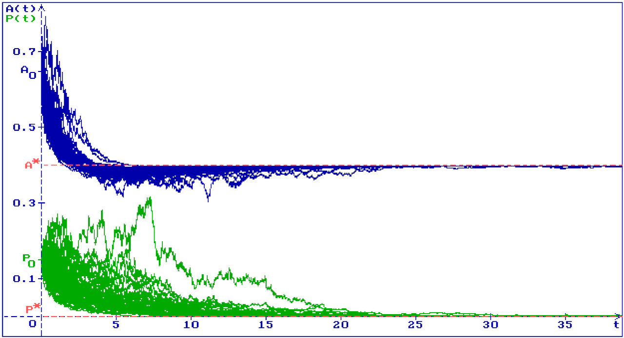
4.2. Equilibrium $E_1$

For system (8), the conditions (13) take the form

$${\displaystyle \frac{1}{2}}{\sigma }_1^2<r_1,{\displaystyle \frac{1}{2}}{\sigma }_2^2+r_2<{\displaystyle \frac{\alpha }{k}}.$$

(16)

So, by conditions (16), the equilibrium $E_1$ is stable in probability.

In Figure 3, three trajectories of the solution of Equation (5) are shown with $r_1=0.6$, $r_2=0.2$, $\mu =0.1$, $k=2.5$, $\alpha =0.9$, $\beta =0.1$, ${\sigma }_1=0.1$, and ${\sigma }_2=0.4$, and different initial conditions: $M_1(0.15,0.4)$, $M_2(0.5,0.6)$, and $M_3(0.9,0.5)$. The conditions (16) hold, and all trajectories converge to the stable equilibrium $E_1=(A^{*},P^{*})$ with $A^{*}=0.4$, and $P^{*}=0$.

Figure 3. Three trajectories of a solution $\left(A\right(t),P(t\left)\right)$ of the system (5) are shown with $r_1=0.6$, $r_2=0.2$, $\mu =0.1$, $k=2.5$, $\alpha =0.9$, $\beta =0.1$, ${\sigma }_1=0.1$, and ${\sigma }_2=0.4$, for different initial conditions: $M_1(0.15,0.4)$, $M_2(0.5,0.6)$, and $M_3(0.9,0.5)$.

In Figure 4, 50 trajectories of the solution of Equation (5) are shown with $A\left(0\right)=0.65$, $P\left(0\right)=0.15$, ${\sigma }_1=0.6$, and ${\sigma }_2=0.4$, and the same values of all other parameters as in Figure 3. All trajectories converge to the stable equilibrium $E_1=(A^{*},P^{*})=(0.4,0)$.

Figure 4. Fifty trajectories $A\left(t\right)$ (blue) and $P\left(t\right)$ (green) of a solution of the system (5) are shown with $r_1=0.6$, $r_2=0.2$, $\mu =0.1$, $k=2.5$, $\alpha =0.9$, $\beta =0.1$, $A\left(0\right)=0.65$, $P\left(0\right)=0.15$, ${\sigma }_1=0.6$, and ${\sigma }_2=0.4$.

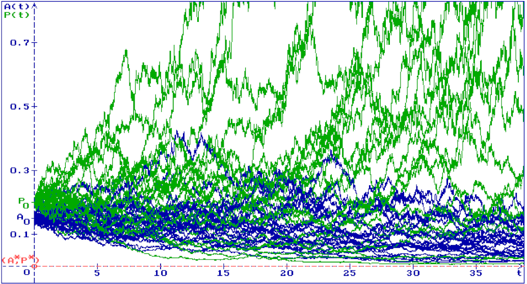
4.3. Equilibrium $E_2$

In the system (9), $a_{22}=0$ and $a_{12}{a}_{21}>0$, i.e., the second condition (14) does not hold. So, in the deterministic case, the equilibrium $E_2$ is unstable.

In Figure 5, three trajectories of the solution $\left(A\right(t),P(t\left)\right)$ of the system (5) are shown with $r_1=0.6$, $r_2=0.21$, $\mu =0.6$, $k=2.5$, $\alpha =0.7$, $\beta =0.1$, ${\sigma }_1=0.12$, ${\sigma }_2=0.03$, $A^{*}=0.3$, and $P^{*}=0.0333$, and different initial conditions: $M_1(0.28,0.035)$, $M_2(0.31,0.035)$, $M_3(0.3,0.031)$. One can see that the all initial conditions are close enough to the equilibrium $(A^{*},P^{*})$, but all trajectories move away from the equilibrium, since this equilibrium is unstable.

Figure 5. Three trajectories of a solution $\left(A\right(t),P(t\left)\right)$ of the system (5) with $r_1=0.6$, $r_2=0.21$, $\mu =0.6$, $k=2.5$, $\alpha =0.7$, $\beta =0.1$, ${\sigma }_1=0.12$, and ${\sigma }_2=0.03$, and initial conditions $M_1(0.28,0.035)$, $M_2(0.31,0.035)$, and $M_3(0.3,0.031).$

In Figure 6, 25 trajectories of the solution of Equation (5) are shown with $A\left(0\right)=0.31$, $P\left(0\right)=0.0433$, ${\sigma }_1=0.1$, and ${\sigma }_2=0.1$, and the same values of all other parameters as in Figure 5. All trajectories move away from the equilibrium $E_2=(A^{*},P^{*})=(0.3,0.0333)$, since this equilibrium is unstable.

Figure 6. Twenty-five trajectories $A\left(t\right)$ (blue) and $P\left(t\right)$ (green) of the solution of system (5) with $r_1=0.6$, $r_2=0.21$, $\mu =0.6$, $k=2.5$, $\alpha =0.7$, $\beta =0.1$, $A\left(0\right)=0.31$, $P\left(0\right)=0.0433$, ${\sigma }_1=0.1$, and ${\sigma }_2=0.1$.

Remark 5.

Note that to simulate solutions of the considered Ito stochastic differential equations in Figure 1, Figure 2, Figure 3, Figure 4, Figure 5 and Figure 6, a special algorithm for modeling trajectories of the standard Wiener process was used, as described in [12].

5. Conclusions

Systems of nonlinear differential equations are used to describe mathematical models in many different applications. As a rule, such models can have several equilibria, each of which can be stable or unstable. A simple criterion was proposed in this paper that can define the stability or instability of each considered equilibrium under the presence of stochastic perturbations around of this equilibrium. Additionally, we showed how the classical “stabilization by noise” can be applied for stabilization of an unstable equilibrium. We also showed how the properties of the nonlinear model equilibria under stochastic perturbations can be demonstrated via numerical simulations of solutions of the considered Ito stochastic differential equations. The obtained results can be applied to many other nonlinear models in different applications.

References

- Bueno, D.J.; Casale, C.H.; Pizzolitto, R.P.; Salvano, M.A.; Oliver, G. Physical adsorption of aflatoxin B1 by lactic acid bacteria and Saccharomyces cerevisiae: A theoretical model. J. Food Prot. 2007, 70, 2148–2154. [Google Scholar] [CrossRef]
- Garcia, D.; Ramos, A.J.; Sanchis, V.; Marín, S. Predicting mycotoxins in foods: A review. Food Microbiol. 2009, 26, 757–769. [Google Scholar] [CrossRef] [PubMed]
- Gibson, A.M.; Hocking, A.D. Advances in the predictive modelling of fungal growth in food. Trends Food Sci. Technol. 1997, 8, 353–358. [Google Scholar] [CrossRef]
- Kademi, H.I.; Baba, I.A.; Saad, F.T. Modelling the dynamics of toxicity associated with aflatoxins in foods and feeds. Toxicol. Rep. 2017, 4, 358–363. [Google Scholar] [CrossRef] [PubMed]
- Kademi, H.I.; Saad, F.T.; Ulusoy, B.H.; Baba, I.A.; Hecer, C. Mathematical model for aflatoxins risk mitigation in food. J. Food Eng. 2019, 263, 25–29. [Google Scholar] [CrossRef]
- Molina, M.; Giannuzzi, L. Modelling of aflatoxin production by Aspergillus parasiticus in a solid medium at different temperatures, pH and propionic acid concentrations. Food Res. Int. 2002, 35, 585–594. [Google Scholar] [CrossRef]
- Pitt, R.E. A descriptive model of mold growth and aflatoxin formation as affected by environmental conditions. J. Food Prot. 1993, 56, 139–146. [Google Scholar] [CrossRef] [PubMed]
- Prandini, A.; Sigolo, S.; Filippi, L.; Battilani, P.; Piva, G. Review of predictive models for Fusarium head blight and related mycotoxin contamination in wheat. Food Chem. Toxicol. 2009, 47, 927–931. [Google Scholar] [CrossRef] [PubMed]
- Van Eijkeren, J.C.; Bakker, M.I.; Zeilmaker, M.J. A simple steady-state model for carry-over of aflatoxins from feed to cow’s milk. Food Addit. Contam. 2006, 23, 833–838. [Google Scholar] [CrossRef] [PubMed] [Green Version]
- Zwietering, M.H.; den Besten, H.M. Modelling: One word for many activities and uses. Food Microbiol. 2011, 28, 818–822. [Google Scholar] [CrossRef] [PubMed]
- Gikhman, I.I.; Skorokhod, A.V. Stochastic Differential Equations; Springer: Berlin, Germany, 1972. [Google Scholar]
- Shaikhet, L. Lyapunov Functionals and Stability of Stochastic Functional Differential Equations; Springer Science & Business Media: Berlin, Germany, 2013. [Google Scholar]
- Khasminskii, R.Z. Stochastic Stability of Differential Equations; Springer: Berlin, Germany, 2012; (In Russian, Moscow, Nauka, 1969). [Google Scholar]
- Korobeinikov, A.; Shaikhet, L. Global asymptotic properties of a stochastic model of population growth. Appl. Math. Lett. 2021, 121, 107429. [Google Scholar] [CrossRef]
Publisher’s Note: MDPI stays neutral with regard to jurisdictional claims in published maps and institutional affiliations. |
© 2021 by the author. Licensee MDPI, Basel, Switzerland. This article is an open access article distributed under the terms and conditions of the Creative Commons Attribution (CC BY) license (https://creativecommons.org/licenses/by/4.0/).
Share and Cite
Shaikhet, L. Asymptotic Properties of One Mathematical Model in Food Engineering under Stochastic Perturbations. Mathematics 2021, 9, 3013. https://doi.org/10.3390/math9233013
Shaikhet L. Asymptotic Properties of One Mathematical Model in Food Engineering under Stochastic Perturbations. Mathematics. 2021; 9(23):3013. https://doi.org/10.3390/math9233013
Chicago/Turabian StyleShaikhet, Leonid. 2021. "Asymptotic Properties of One Mathematical Model in Food Engineering under Stochastic Perturbations" Mathematics 9, no. 23: 3013. https://doi.org/10.3390/math9233013
APA StyleShaikhet, L. (2021). Asymptotic Properties of One Mathematical Model in Food Engineering under Stochastic Perturbations. Mathematics, 9(23), 3013. https://doi.org/10.3390/math9233013