Randomized Projection Learning Method for Dynamic Mode Decomposition

Abstract

A data-driven analysis method known as dynamic mode decomposition (DMD) approximates the linear Koopman operator on a projected space. In the spirit of Johnson–Lindenstrauss lemma, we will use a random projection to estimate the DMD modes in a reduced dimensional space. In practical applications, snapshots are in a high-dimensional observable space and the DMD operator matrix is massive. Hence, computing DMD with the full spectrum is expensive, so our main computational goal is to estimate the eigenvalue and eigenvectors of the DMD operator in a projected domain. We generalize the current algorithm to estimate a projected DMD operator. We focus on a powerful and simple random projection algorithm that will reduce the computational and storage costs. While, clearly, a random projection simplifies the algorithmic complexity of a detailed optimal projection, as we will show, the results can generally be excellent, nonetheless, and the quality could be understood through a well-developed theory of random projections. We will demonstrate that modes could be calculated for a low cost by the projected data with sufficient dimension.

1. Introduction

Modeling real-world phenomena in physical sciences to engineering, videography, and economics is limited due to computational costs. Real-world systems require dynamic nonlinear modeling. Dynamic mode decomposition (DMD) [1,2,3] is an emerging tool in this area that could use the data directly rather than intermediary differential equations. However, the data in real-world applications is enormous. The DMD algorithm’s reliance on a singular value decomposition (SVD) appears to be a limiting factor due to storing and calculating the SVD of such a matrix. One can notice that SVD calculations of snapshot matrices in big projects would require the use of supercomputers or days of computation. To allow processing on small-scale computers and in a shorter time frame, we propose developing an algorithm based on a randomized projection [4], which is used to reduce the dimension of observable space in DMD, which we call rDMD. In order to utilize and carefully analyzed the rDMD, we will use the Johnson–Lindenstrauss lemma. It is clear that a random projection is simple as compared to a detailed optimal projection method, but our analysis and examples demonstrate, nonetheless, the quality and efficiency.

Strong theoretical support from Johnson–Lindenstrauss(JL) lemma [5] makes the random projection method reliable and has extensive utilization in the field of data science. According to the JL lemma, if data points lie in a sufficiently high-dimensional space, then those data points may be projected into a sufficiently low-dimensional space while approximately preserving the distance of the data points. Furthermore, the projection can be done by a random matrix, which makes algorithms based on the JL lemma both past and simple. Hence, this tool is more powerful and adopted heavily in data science. JL lemma-based random projection and SVD-based projection can be used to project N dimensional data into a lower dimension $L<<N$. Data matrix $X_{N\times M}$ can be projected (by random projection) into a lower dimension (L) subspace as $X_L:=RX$, where R is a random matrix with unit length. Hence, the random projection is very simple because it relies only on matrix multiplication. Moreover, computational complexity is $\mathcal{O}\left(MLN\right)$, while SVD has computational complexity $\mathcal{O}\left(N{M}^2\right)$ when $M<N$ [6]. We will use the random projection to project high-dimensional snapshot matrices into a manageable low-dimensional space. In a theoretical perspective, the dimensions of the input and output spaces in the Koopman operator can be reduced by the random projection method; thus, reducing the storage and computational cost of the DMD algorithm.

Both DMD [2] and rDMD are grounded in theory through the application of the Koopman operator. They are numerical methods used to estimate the Koopman operator that identifies spatial and temporal patterns from a dynamical system. Theoretical support of the Koopman operator theory makes the these algorithms strong. A major objective of the DMD method is to isolate and interpret the spatial features of a dynamical system through the associated eigenvalues of the DMD operator (see Section 4.3). Our new randomized DMD (rDMD) algorithm targets to address issues that arise in SVD-based existing DMD methods by reducing the dimensionality of the matrix just by using matrix multiplication. rDMD can achieve very accurate results with low-dimensional data embedded in high-dimensional observable space.

This paper will summarize the Koopman operator theory, existing DMD algorithms, and random projection theory in Section 2. Then we will discuss our proposed randomized DMD algorithm in Section 3, and finally, in Section 4, we will provide examples that support our approach. Major notations and abbreviations used in this article are listed in Table 1.

Table 1. Major notations and abbreviations used in the article.

Notation and Abbreviations	Meaning
$\mathcal{K}$	Koopman operator
M	Number of snapshots
N	Number of observable
L	Dimension of the projected observable space
$\mathbb{K}$	DMD on original space
$\widehat{\mathbb{K}}$	DMD on projected space
X	Snapshot matrix: time stape 0 to M
Y	Snapshot matrix: time stape 0 to M
$X_L,Y_L$	Projected snapshot matrices
P	Projection matrix of dimension $L\times N$
R	Random projection matrix
$(\lambda ,\varphi )$	Eigenvalue and eigenvector of $\mathbb{K}$
$({\lambda }_L,{\varphi }_L)$	Eigenvalue and eigenvector of $\widehat{\mathbb{K}}$
DMD	Dynamic Mode Decomposition
SVD	Extended Dynamic Mode Decomposition
rDMD	randomized Dynamic Mode Decomposition
RP	Random Projection
JL	Johnson–Lindenstrauss

Remark 1

(Problem Statement). In this article, we investigate the estimation of Koopman modes by the computationally efficient method. Standard existing methods calculate the SVD of the snapshot matrix. However, direct SVD calculations of such matrices can be quite large and computationally intensive. Here, we propose a simple method based on the JL lemma to perform calculations simply on random subsamples, doing so in an analytically rigorous and controlled way. In addition, we will generalize the current SVD-based methods as a DMD in a projected space. This allows extension of choices that can be used in DMD algorithms. We will show the quality of our theoretical results through the well-developed theory of random projections in high-dimensional geometry. In addition, experimental and real-world examples validate excellent results with the theory underlying our method.

2. Dynamic Mode Decomposition and Background Theory

The focus of this paper is to approximate the eigenpairs of the Koopman operator based on the randomized dynamic mode decomposition method. We will first review the underlining theory about the Koopman operator.

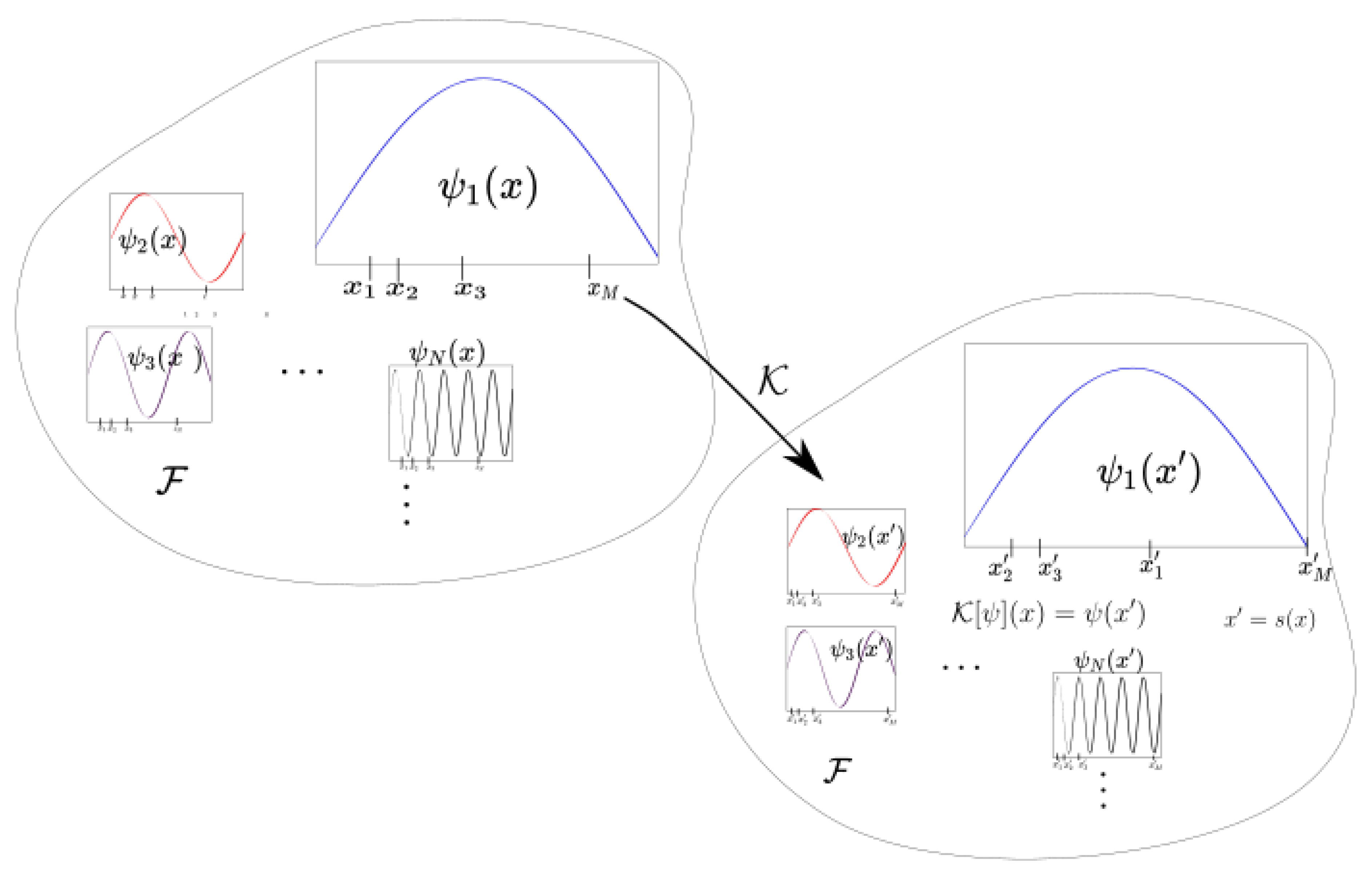
2.1. Koopman Operator

Consider a discrete-time dynamical system

$$\begin{array}{c}\hfill x_{n+1}=S\left(x_n\right),\end{array}$$

(1)

where $S:\mathcal{M}\to \mathcal{M}$ and $\mathcal{M}$ is a finite dimensional manifold. (If we have a differential equation or continuous time dynamical system, the flow map can be considered.) The variable x is often recognized as a state variable and $\mathcal{M}$ as phase space. The associated Koopman operator is described as the evaluation of observable functions (Figure 1) $\psi :\mathcal{M}\to \mathbb{R}$ in function space $\mathcal{F}$. Instead of analyzing the individual trajectories in phase space, the Koopman operator operates on the observations [2,3,7,8].

Figure 1. This figure shows the behavior of the Koopman operator $\mathcal{K}$ in observable space $\mathcal{F}$ associated with a dynamical system S. The Koopman operator evaluates the observable $\psi$ at downstream or future $x^{\prime }=x_{n+1}=s\left(x_n\right)$.

Definition 1

(Koopman operator [7]). The Koopman operator $\mathcal{K}$ for a map S is defined as the following composition,

$$\begin{array}{cc}\hfill \mathcal{K}& :\mathcal{F}\to \mathcal{F}\hfill \\ \hfill \psi \mapsto \mathcal{K}\left[\psi \right]& =\psi \circ S\hfill \end{array}$$

(2)

on the function space $\mathcal{F}$.

It is straightforward, to prove [7],

$$\begin{array}{c}\hfill \mathcal{K}[a{\psi }_1+b{\psi }_2]=a({\psi }_1\circ S)+b({\psi }_2\circ S)=a\mathcal{K}\left[{\psi }_1\right]+b\mathcal{K}\left[{\psi }_2\right]\end{array}$$

(3)

for ${\psi }_1,{\psi }_2\in \mathcal{F}$ and $a,b\in \mathbb{C}$ and, therefore, the Koopman operator is linear on $\mathcal{F}$. This is an interesting and important property of the operator because the associated map S most probably will be non-linear. Even though the operator is associated with a map that evolves in a finite dimensional space, $\mathcal{F}$ the function space in which the operator acts on could possibly be an infinite dimensional. This is the trade-off between costs for the linearity [8].

Spectral analysis of the Koopman operator can be used to decompose the dynamics, which is the key success in the DMD. Assuming the spectrum of the Koopman operator $\mathcal{K}$ is given by

$$\begin{array}{c}\hfill \mathcal{K}{\psi }_i\left(x\right)={\lambda }_i{\psi }_i\left(x\right)i=1,2,3,\cdots \end{array}$$

(4)

then vector-valued observables $\mathit{g}:\mathcal{M}\to {\mathbb{R}}^N$(or ${\mathbb{C}}^N$) can be represented by

$$\begin{array}{c}\hfill \mathit{g}\left(\mathit{x}\right)=\sum _{i=1}^{\infty }{\psi }_i\left(\mathit{x}\right){\mathit{\varphi }}_{\mathit{i}},\end{array}$$

(5)

where ${\mathit{\varphi }}_{\mathit{i}}\in {\mathbb{R}}^N$(or ${\mathbb{C}}^N$) are the vector coefficients of the expansion and called “Koopman modes”(here we assumed that components of $\mathit{g}$ lie within the span of the eigenfunctions of $\mathcal{K}$). Note that the observable value at time $n+1$ is given by

$$\begin{array}{c}\hfill \mathit{g}\left({\mathit{x}}_{\mathit{n}+\mathbf{1}}\right)=\sum _{i=1}^{\infty }{\lambda }_i^n{\psi }_i\left({\mathit{x}}_{\mathbf{0}}\right){\mathit{\varphi }}_{\mathit{i}}.\end{array}$$

(6)

This decomposition can be used to separate the spacial and time components of the dynamical system and can be used to isolate the specific dynamics.

2.2. Dynamic Mode Decomposition

The dynamic mode decomposition is a data-driven method to estimate the Koopman modes from numerical or experimental data [2]. Suppose dynamics are governed by Equation (1) for any state $\mathit{x}$ and vector valued measurements are given by observable $\mathit{g}\left(\mathit{x}\right)\in {\mathbb{R}}^N$. For a given set of data $X=[\mathit{g}\left({\mathit{x}}_{\mathbf{0}}\right)\mathit{g}\left({\mathit{x}}_{\mathbf{1}}\right)\cdots \mathit{g}\left({\mathit{x}}_{\mathit{M}-\mathbf{1}}\right)],Y=[{\mathit{y}}_{\mathbf{0}}{\mathit{y}}_{\mathbf{1}}\cdots {\mathit{y}}_{\mathit{M}-\mathbf{1}}]$ where ${\mathit{y}}_{\mathit{i}}=\mathit{g}\left(\mathit{s}\left({\mathit{x}}_{\mathit{i}}\right)\right)$, the Koopman modes and eigenvalues of the Koopman operator can be estimated through solving the least-squares problem

$$\begin{array}{c}\hfill \mathbb{K}=\underset{K}{arg\; min}\left|\right|KX-{Y\left|\right|}_F^2=\underset{K}{arg\; min}\sum _{i=0}^{M-1}\left|\right|K\mathit{g}\left({\mathit{x}}_{\mathit{i}}\right)-{\mathit{y}}_{\mathit{i}}{\left|\right|}_2^2\end{array}$$

(7)

and $\mathbb{K}=Y{X}^{†}$ (here $X^{†}$ is the pseudo-inverse of X) is defined as the “Exact DMD” operator [3]. The eigenvalue ($\widehat{\lambda }$) of $\mathbb{K}$ is an approximation of an eigenvalue ($\lambda$) of $\mathcal{K}$; the corresponding right eigenvector($\widehat{\varphi }$) is called the DMD mode and approximates the Koopman mode ($\varphi$). Then the observable value $\mathit{g}\left(\mathit{x}\right(\mathit{t}\left)\right)$ at time t can be modeled as

$$\begin{array}{c}\hfill \mathit{g}\left(\mathit{x}\left(\mathit{t}\right)\right)=\sum _{i=1}^r{\psi }_i\left({\mathit{x}}_{\mathbf{0}}\right){\widehat{\mathit{\varphi }}}_{\mathit{i}}{\widehat{\lambda }}_i^t\end{array}$$

(8)

where r is the number of selected DMD modes and demonstrates the finite dimensional approximation for vector-valued observable $\mathit{g}$ under the Koopman operator. Based on this decomposition, data matrices can be expressed as

$$\begin{array}{cc}\hfill X_{N\times M}& ={\Phi }_{N\times r}{T}_{r\times M}\hfill \\ \hfill Y_{N\times M}& ={\Phi }_{N\times r}{\Lambda }_{r\times r}{T}_{r\times M}\hfill \end{array}$$

(9)

where $\Phi =[{\psi }_1\left(x_0\right){\mathit{\varphi }}_1{\psi }_2\left(x_0\right){\mathit{\varphi }}_2\cdots {\psi }_r\left(x_0\right){\mathit{\varphi }}_r]$, T is a Vandermonde matrix with $T_{ij}={\lambda }_i^{j-1}$ for $i=1,2,\cdots r$, $j=1,2,\cdots ,M$ and $\Lambda =diag\{{\lambda }_1,{\lambda }_2,\cdots ,{\lambda }_r\}$. Note that with the above decomposition $\mathbb{K}=Y{X}^{†}=\Phi \Lambda T{T}^{†}{\Phi }^{†}$. We will suppose $\mathbb{K}$ has distinct eigenvalues ${\lambda }_i$, columns of X are linearly independent and $r\le M$. In practical applications, we are expected to fully understand the data set by relatively few ($r<<M$) modes. This can be considered one of the dimension reduction steps of the algorithm. Additionally, the dimension of columns of the data matrix need to be reduced.

In practice, the columns of data matrix X (and Y) are constructed by the snapshot matrices of spatial observable data. More often, those snapshots lie in a high-dimensional space ${\mathbb{R}}^N$ ($N>>1$ and roughly $\mathcal{O}\left({10}^{15}\right)$ to $\mathcal{O}\left({10}^{10}\right)$), but the number of snapshots or time steps (M) are small and often it is $\mathcal{O}\left({10}^3\right)$ to $\mathcal{O}\left({10}^1\right)$ [9]. Hence, computing the spectrum of matrix $\mathbb{K}$ by direct SVD is computationally intensive, even though most of the eigenvalues will be zero. Method-of-snapshot, parallel version of SVD, or randomized SVD can be used to attack this difficulty [10,11]. In this project, we use a more simple randomized method by generalizing the DMD algorithm. We can project our data matrices $X,Y$ into a low-dimensional space $R^L$ with $r\le L\le M<<N$; therefore, we need to estimate the spectrum of $\mathbb{K}$ based on the computation on the projected space. Our proposed rDMD method is focused on this dimension reduction step.

In the next section (Section 3), we will discuss more details about the calculation. Note that the current methods are based on the singular value decomposition of the data matrix X to construct a projection, and our proposed algorithm is based on the random projection method to project data into a low-dimensional space.

2.3. Random Projection

The random projection method is based on the Johnson–Lindenstrauss lemma, which is applied by many data analysis methods. In this article, we use a random matrix R generated by a Gaussian distribution, such that each element $r_{ij}\stackrel{iid}{\sim }\mathcal{N}(0,1)$ with a normalize column is of unit length.

Theorem 1

(Johnson–Lindenstrauss lemma [5]). For any $0<ϵ<1$ and any integer $M>1,$ let L be a positive integer, such that $L\ge L_0$ with $L_0=\frac{ClnM}{{ϵ}^2},$ where C is a suitable constant ($C\approx 8$ in practice, $C=2$ is good enough). Then for any set X of M data points in ${\mathbb{R}}^N$, there exists a map $f:{\mathbb{R}}^N\to {\mathbb{R}}^L$ such that for all $x_1,x_2\in X$,

$$(1-ϵ)\left|\right|x_1-x_2{\left|\right|}^2\le \left|\right|f\left(x_1\right)-f\left(x_2\right){\left|\right|}^2\le (1+ϵ)\left|\right|x_1-x_2{\left|\right|}^2.$$

Theorem 2

(Random Projection [4]). For any $0<ϵ,\delta <\frac{1}{2}$ and positive integer N, there exists a random matrix R of size $L\times N$ such that for $L\ge L_0$ with $L_0=\frac{Cln(1/\delta )}{{ϵ}^2}$. and for any unit-length vector $x\in R^N$

$$Pr\left\{\right|\left|\right|Rx|{|}^2-1|>ϵ\}\le \delta$$

or

$${Pr\left\{\right|\left|\right|Rx\left|\right|}^2-1|>ϵ\}\le e^{-CL{ϵ}^2}$$

A low rank approximation for both $X,Y$ can be found using the random projection method. Notice that both these matrices have M points from N dimensional observable space and, therefore, we can use random projection matrix R of size $L\times N$ with the $L\ge \frac{ClnN}{{ϵ}^2}$, which provides $ϵ-$ isometry to ${\mathbb{R}}^N$. (See Figure 2 for details).

Figure 2. DMD operator on the projected space. This figure shows the relationship between the DMD operator on original space and DMD on projected space. The operator $\widehat{\mathbb{K}}$ on the projected space is defined in Equation (10) and can be calculated by Equation (10).

3. Randomized Dynamic Mode Decomposition

In this section, we generalize currently used DMD algorithms and then discuss our proposed randomized DMD algorithm.

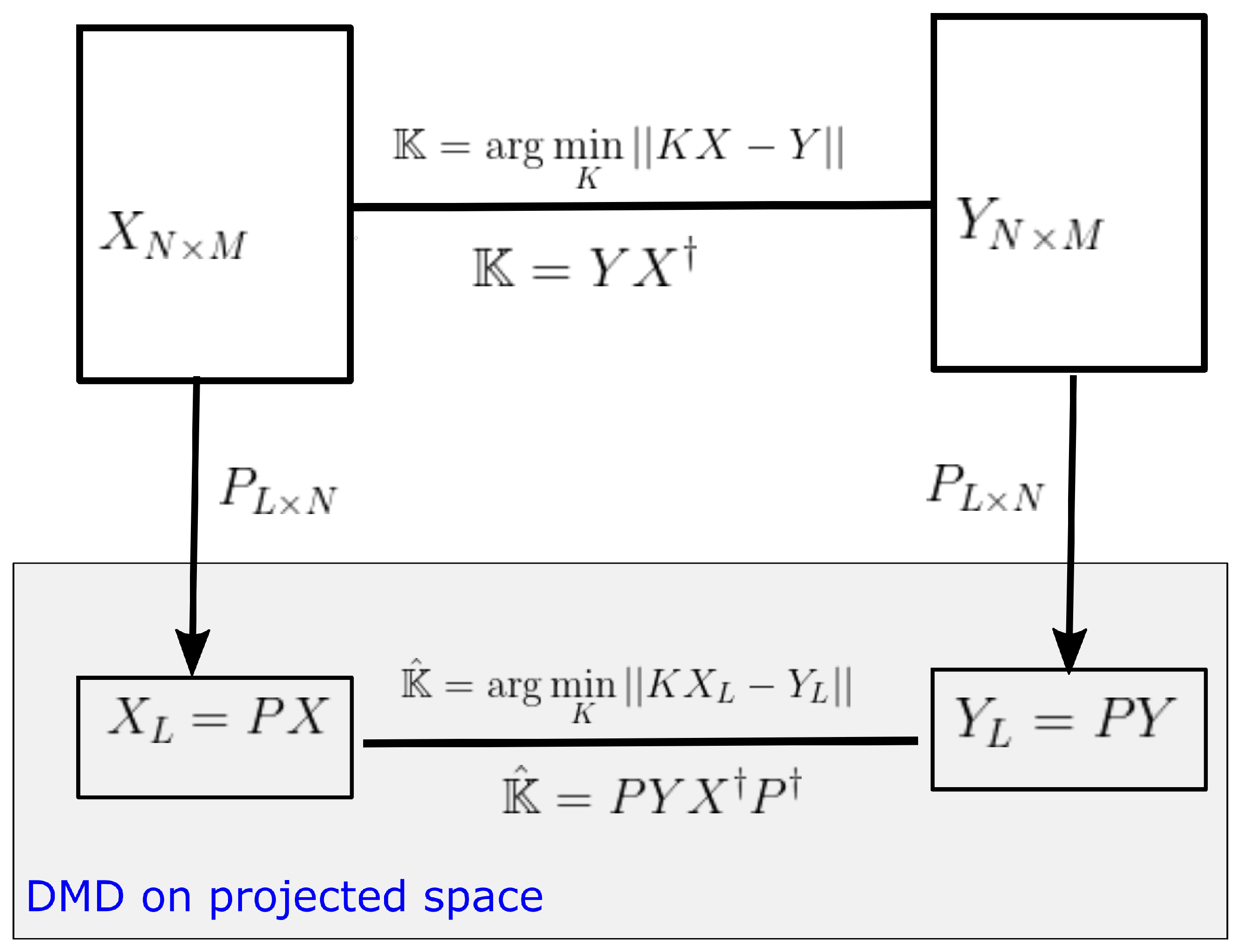
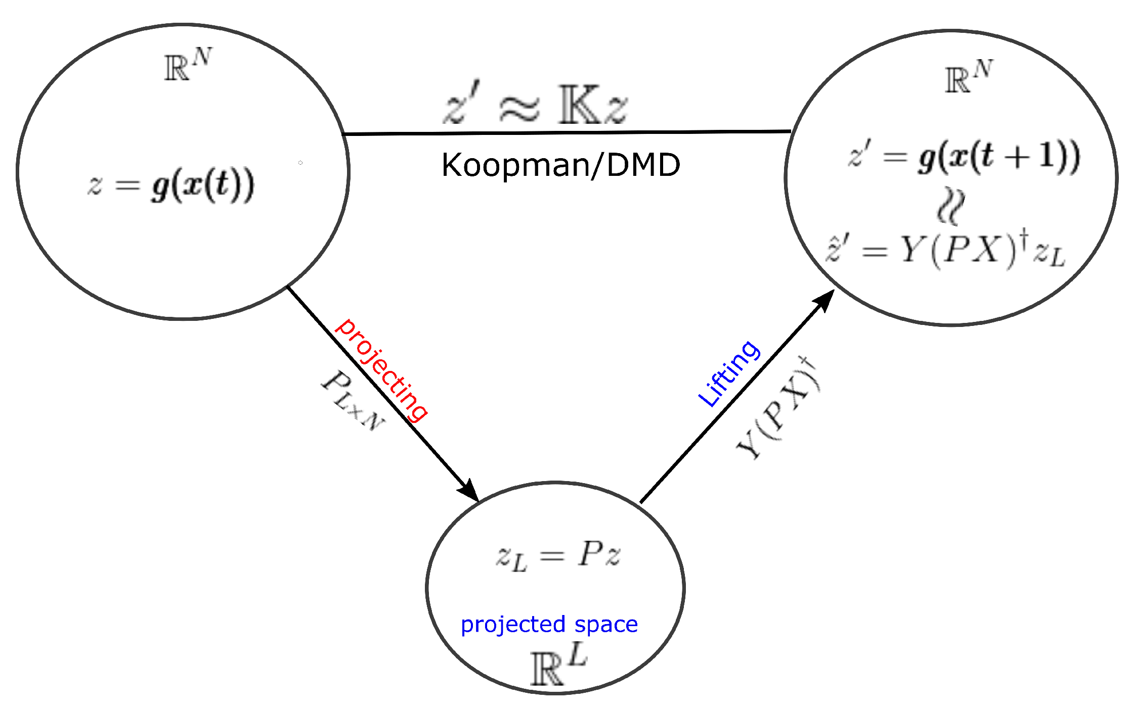
3.1. DMD on Projected Space

As mentioned in Section 2.2, computational and storage costs of DMD can be reduced by projecting data into a low-dimensional observable space. Let $P\in {\mathbb{R}}^{L\times N}$ be any rank L projection matrix, then dimension of data matrices $X,Y\in {\mathbb{R}}^{N\times M}$ can be reduced to $L\times M$ by the projection $X_L=PX,Y_L=PY$. The DMD operator on the projected space (see Figure 2) is given by,

$$\begin{array}{c}\hfill \widehat{\mathbb{K}}=\underset{K\in {\mathbb{R}}^{L\times L}}{arg\; min}\left|\right|K{X}_L-Y_L{\left|\right|}_F^2=\underset{K\in {\mathbb{R}}^{L\times L}}{arg\; min}\left|\right|KPX-{PY\left|\right|}_F^2\end{array}$$

(10)

and $\widehat{\mathbb{K}}=PY{\left(PX\right)}^{†}$. Therefore

$$\begin{array}{c}\hfill \widehat{\mathbb{K}}=PY{\left(PX\right)}^{†}=PY{X}^{†}{P}^{†}=P\mathbb{K}{P}^{†}\end{array}$$

(11)

where $\mathbb{K}=Y{X}^{†}$ is the DMD operator on the original space.

Proposition 1.

Some eigenpairs $(\lambda ,\varphi )$ of $\mathbb{K}$ can be obtain by $({\lambda }_L,{\varphi }_L)$ of projected DMD $\widehat{\mathbb{K}}$ with $\lambda ={\lambda }_L$ and $\varphi =P^{†}{\varphi }_L$.

Proof. 

Let $({\lambda }_L,{\varphi }_L)$ be an eigenpair of $\widehat{\mathbb{K}}$. Then $\widehat{\mathbb{K}}{\varphi }_L={\lambda }_L{\varphi }_L$ and by Equation (11), $P\mathbb{K}{P}^{†}{\varphi }_L={\lambda }_L{\varphi }_L$. Now let $P^{†}{\varphi }_L=\varphi$, then ${\varphi }_L=P\varphi$ because $P{P}^{†}=I$. Hence, $P\mathbb{K}{P}^{†}{\varphi }_L=P\mathbb{K}\varphi ={\lambda }_{L}P\varphi$ and $P(\mathbb{K}\varphi -{\lambda }_L\varphi )=0$. Since $\mathbb{K}\varphi -{\lambda }_L\varphi =0$ is a solution to the above equation, ${\lambda }_L$ is an eigenvalue and the corresponding eigenvector is $\varphi =P^{†}{\varphi }_L$ of $\mathbb{K}$.    □

In other words, we can lift up the dimension of eigenvectors in a projected space by $P^{†}$ to obtain an eigenvector in the original data space. However to avoid the direct calculation of the pseudo-inverse of the projection matrix, we can calculate the eigenvector in the output space $Y_L$ of the DMD operator and lift up the vector into the original output space Y. We can easily show that $\widehat{\varphi }=Y{\left(PX\right)}^{†}{\varphi }_L$ is an eigenvector of $\mathbb{K}$ for corresponding non-zero eigenvalues.

$$\begin{array}{cc}\hfill \mathbb{K}\widehat{\varphi }& =\mathbb{K}Y{\left(PX\right)}^{†}{\varphi }_L=\mathbb{K}Y{X}^{†}{P}^{†}{\varphi }_L\hfill \\ \hfill & =\mathbb{K}\mathbb{K}{P}^{†}{\varphi }_L\hfill \\ \hfill & =\mathbb{K}\lambda P^{†}{\varphi }_L\hfill \\ \hfill & =\lambda Y{X}^{†}{P}^{†}{\varphi }_L\hfill \\ \hfill & =\lambda Y{\left(PX\right)}^{†}{\varphi }_L\hfill \\ \hfill & =\lambda \widehat{\varphi }\hfill \\ \hfill \end{array}$$

(12)

Moreover, notice, $P\widehat{\varphi }=PY{\left(PX\right)}^{†}{\varphi }_L=\widehat{\mathbb{K}}{\varphi }_L$ and, therefore, $\widehat{\varphi }$ estimates the eigenvector on the output space Y. A detailed view of this lifting operator is shown in Figure 3. It provides the relationship of the lifting operator with the DMD operator acting on any general observable vector $z=\mathit{g}\left(\mathit{x}\left(\mathit{t}\right)\right)\in {\mathbb{R}}^N$.

Figure 3. The figure shows the projecting operator P and DMD related lifting operator $Y{\left(PX\right)}^{†}=\mathbb{K}{P}^{†}$, which should be used in DMD algorithms. Instead of using $P^{†}$ as the lifting operator, $Y{\left(PX\right)}^{†}$ can be used for efficient calculations. Moreover, notice that ${\widehat{z}}_L^{\prime }:=P{\widehat{z}}^{\prime }=\widehat{\mathbb{K}}{z}_L$.

Next, the focus moves to the spatial–temporal decomposition of the projected data matrices by spectrum of the DMD operator. Note that the observable value $\mathit{g}\left(\mathit{x}\right(\mathit{t}\left)\right)$ at time t can be modeled as $\mathit{g}\left(\mathit{x}\left(\mathit{t}\right)\right)={\sum }_{i=1}^r{\psi }_i\left({\mathit{x}}_{\mathbf{0}}\right)P^{†}{\left({\mathit{\varphi }}_{\mathit{L}}\right)}_i{\widehat{\lambda }}_i^t$ and similar to the Equation (9), data can be decomposed as

$$\begin{array}{cc}\hfill X_{N\times M}& =P_{N\times L}^{†}{\tilde{\Phi }}_{L\times r}{T}_{r\times M}\hfill \\ \hfill Y_{N\times M}& =P_{N\times L}^{†}{\tilde{\Phi }}_{L\times r}{\Lambda }_{r\times r}{T}_{r\times M}.\hfill \end{array}$$

(13)

This decomposition leads to $\mathbb{K}=Y{X}^{†}=P^{†}\tilde{\Phi }\Lambda T{T}^{†}{\tilde{\Phi }}^{†}P$ and if $r\le L$ all the non-zero eigenvalues and corresponding eigenvectors of $\mathbb{K}$ can be constructed by the projected DMD operator. Further, Equation (13) can be use to isolate the spatial profile of interesting dynamical compotes, such as attractors, periodic behaviors, etc.

Based on the choice of the projection matrix, we have alternative ways to estimate the spectrum of the DMD operator.

Remark 2

(Projection by SVD). A commonly used projection matrix is based on SVD of the input matrix $X=U\Sigma V^{*}$ and the projection matrix is chosen to be $P=U^{*}$, here, ${}^{*}$ represents the conjugate transpose of a matrix. Using Equation (11) and SVD of X, the operator on the projected space can be formulated as $\widehat{\mathbb{K}}=U^{*}YV{\Sigma }^{-1}$.

Remark 3

(Standard DMD and Exact DMD). Let eigenpair of an SVD-based $\widehat{\mathbb{K}}=U^{*}YV{\Sigma }^{-1}$ be given by $(\lambda ,{\varphi }_L)$. In a standard DMD (Reference Schmid’s paper and Tu’s paper) use the eigenvector $P^{†}{\varphi }_L=U{\varphi }_L$ to estimate eigenvectors of $\mathbb{K}$. On the other hand, in the exact DMD (reference Tu’s paper) this eigenvector is estimated by $Y{\left(PX\right)}^{†}{\varphi }_L=YV{\Sigma }^{-1}{\varphi }_L$.

Remark 4.

One can also use QR decomposition-based projection methods. QR decomposition of the input–output snapshot data matrix $\left[XY\right]$ is used in some existing methods [3], and so our philosophy of random projection methods used here will greatly improve efficiency, but, nonetheless, with quality that is controlled in an analytically rigorous way.

In this paper, we propose a simple random projection-based method to estimate the spectrum of the DMD operator.

3.2. Randomized Methods

Our suggested randomized dynamic mode decomposition(rDMD) is based on the random projection applied to the theory of DMD on a projected space. We can reduce the dimension of the data matrix $X,Y$ in DMD by using a random projection matrix $R_{L\times N}$. In other words, we construct a projection matrix P discussed in Section 3.1 as a random matrix R whose columns have unit lengths and entries that are selected independently and identically from a probability distribution. Therefore, the rDMD matrix on the projected space is given by $\widehat{\mathbb{K}}=RY{\left(RX\right)}^{†}$, and if an eigenpair of $\widehat{\mathbb{K}}$ is given by $(\lambda ,{\varphi }_L)$, then the eigenpair of $\mathbb{K}$ is given $(\lambda ,Y{\left(RX\right)}^{†}{\varphi }_L)$. Algorithm 1 represents the major steps needed to estimate the eigenvalues and corresponding eigenvectors of the DMD operator with the random projection method.In addition, Figure 4 shows the details of the input–output variables of the algorithm, spatiotemporal decomposition of the data, and how to use the eigendecomposition of the Koopman operator to isolate and interpret the spatial features of a dynamical system.

Figure 4. The figure summarize the rDMD algorithm, its input data, and the output variables. This also explains how to use the eigendecomposition of the Koopman operator to isolate and interpret the spatial features of a dynamical system. This figure is new from the previous manuscript.

The calculation of the projection matrix of a standard or exact DMD algorithm based on the SVD of the snapshot matrix X is needed to store a full high-resolution data matrix, which leads to memory issues. Our proposed rDMD algorithm can avoid these storage issues, because low-dimensional matrices $X_L,Y_L$ obtained by matrix multiplications only need to store one row and one column of each matrix at a time. Additionally, this algorithm reduces the computational cost, since we only need to calculate the pseudo-inverse of comparatively lower dimensional matrix. The choice of the distribution of R can further reduce the computational cost [12].

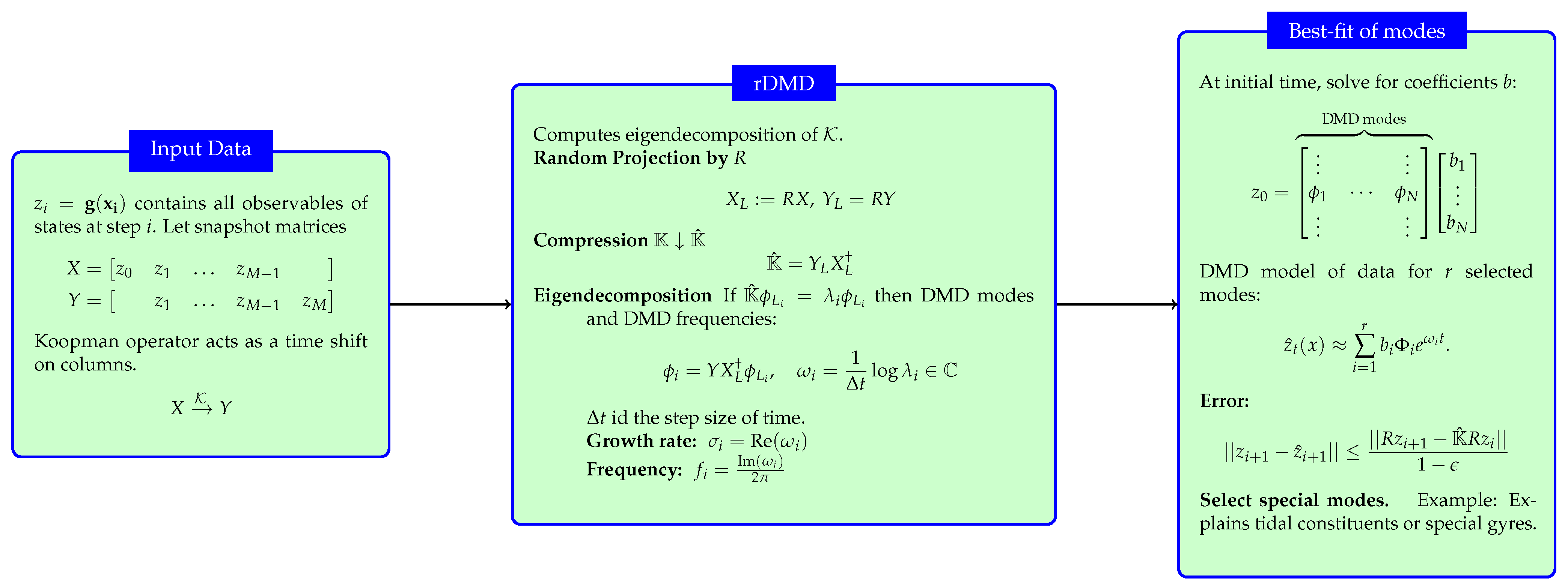
Algorithm 1 Randomized DMD (rDMD). Figure 4 shows the details of the input and output variable

Data: $X,Y\in {\mathbb{R}}^{N\times M}$ Input: $ϵ$ $L_0=\frac{ClnM}{{ϵ}^2}$; Choose L such that $L\ge L_0$; Construct a random matrix $R=\frac{1}{\sqrt{L}}\left(r_{ij}\right)\in {\mathbb{R}}^{L\times N}$ such that $r_{ij}\sim \mathcal{N}(0,1)$; Calculate $X_L:=RX,Y_L:=RY$; Calculate $\widehat{\mathbb{K}}=Y_L{X}_L^{†}$; [$\Lambda$${\Phi }_L$]=eigs($\widehat{\mathbb{K}}$); Result: $diag(\Lambda )$, $Y{X}_L^{†}{\Phi }_L$

One time step forecasting error for any given snapshot by using the rDMD algorithm can be bounded by using the JL theory.

Theorem 3

(Error Bound). Let $z=\mathit{g}\left(\mathit{x}\left(\mathit{t}\right)\right),z^{\prime }=\mathit{g}\left(\mathit{x}(\mathit{t}+\mathbf{1})\right)\in {\mathbb{R}}^N$. Error bound of estimating $z^{\prime }$ by using the rDMD as ${\widehat{z}}^{\prime }=Y{X}^{†}{R}^{†}Rz$ is given by

$$\begin{array}{c}\hfill E(z^{\prime };L):=\left|\right|z^{\prime }-{\widehat{z}}^{\prime }\left|\right|\le \frac{\left|\right|R{z}^{\prime }-\widehat{\mathbb{K}}Rz\left|\right|}{1-ϵ}:=UB\end{array}$$

(14)

with at least the probability of $\mathcal{O}(1/M^2)$ for any $0<ϵ<1$ with $L>\frac{Clog\left(M\right)}{{ϵ}^2}$.

Proof. 

Since $\widehat{\mathbb{K}}=RY{X}^{†}{R}^{†}$, the rDMD acts on the projected vector, which can be rearranged as $\widehat{\mathbb{K}}Rz=R{\widehat{z}}^{\prime }$. Therefore,

$$\begin{array}{c}\hfill \left|\right|R{z}^{\prime }-\widehat{\mathbb{K}}Rz\left|\right|=\left|\right|R{z}^{\prime }-R{\widehat{z}}^{\prime }\left|\right|.\end{array}$$

Now we can apply the JL theory to attain the desired error bound.

$$\begin{array}{c}\hfill (1-ϵ)\left|\right|z^{\prime }-{\widehat{z}}^{\prime }\left|\right|\le \left|\right|R{z}^{\prime }-R{\widehat{z}}^{\prime }\left|\right|=\left|\right|R{z}^{\prime }-\widehat{\mathbb{K}}Rz\left|\right|.\end{array}$$

Hence $\left|\right|z^{\prime }-{\widehat{z}}^{\prime }\left|\right|\le \frac{\left|\right|R{z}^{\prime }-\widehat{\mathbb{K}}Rz\left|\right|}{1-ϵ}$. □

4. Results and Discussion

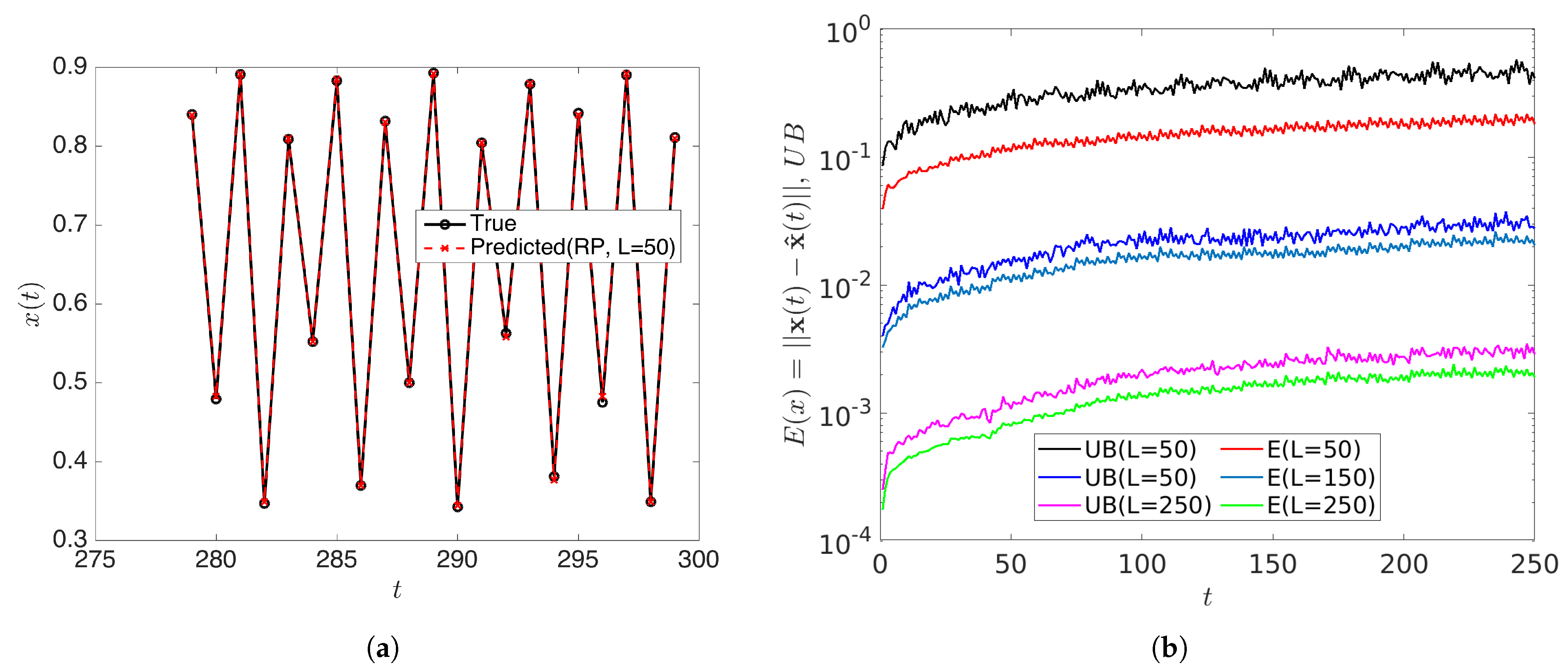
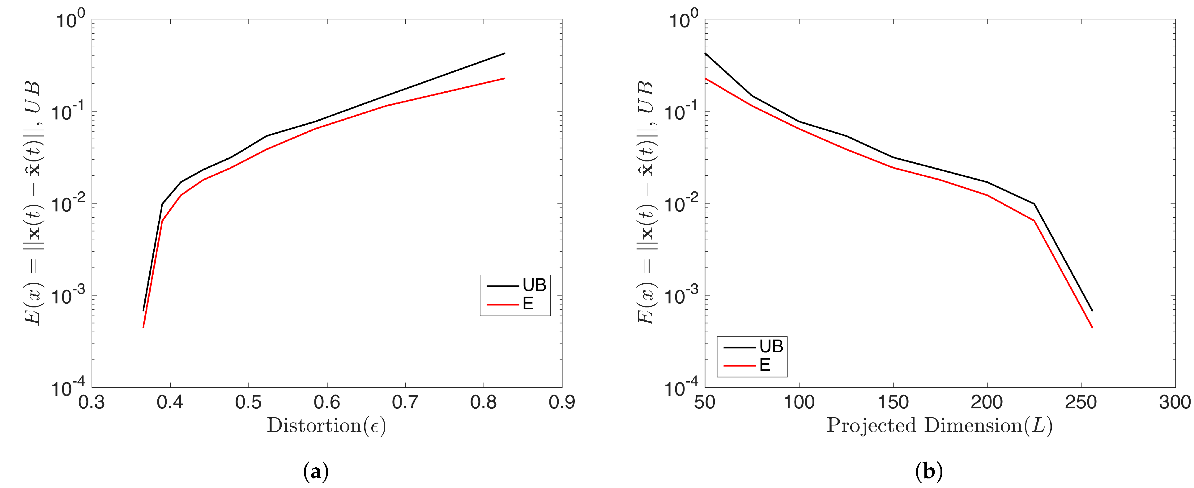
In this section, we demonstrate the theory of rDMD with a few examples. The first two examples consider the computation for known dynamics and demonstrate the error analysis. The final example demonstrates application in the field of oceanography and isolates the interesting features by rDMD, compering the resulting modes with the exact DMD results.

4.1. Logistic Map

We first consider a dataset of 300 snapshots from a logistic map,

$$\begin{array}{c}\hfill x_{n+1}=a{x}_n(1-x_n)\end{array}$$

with $a=3.56994$. In this case, all initial conditions will converge to a period-256 orbit. Therefore the rank of the snapshot matrix with relatively high samples should be 256. We forecasted the data by using the rDMD method and then analyzed the error of the prediction and compared it with the theoretical upper bound. With $N=5000$ initial conditions and $M=300$ samples, the dimension L of the projecting space can be chosen as $L\ge \frac{Cln\left(300\right)}{{ϵ}^2}\approx \frac{34.22}{{ϵ}^2}$ when $C=6$. rDMD with projection into a 50 dimensional space can accurately forecast the time series data. (Figure 5 shows the original vs. predicted data for one trajectory.) Furthermore, Figure 6 demonstrates the bound of the error of the forecast explained in Equation (14) and how the error relates to the distortion parameter $ϵ$ (Figure 6a) and the dimension of the projected space (Figure 6b). Since the rank of the snapshot matrix is 256, any $L\ge 256$ will perform very accurately. This example validates the error bound we discussed in Equation (14) and the error of the prediction depends on the error exhibited by the projected DMD operator and the distortion parameter ($ϵ$ or the projected dimension) from the JL theory.

Figure 5. (a) Shows the predicted data using the rDMD algorithm with projected dimension $L=50$ compared to the original data from logistic map $x_{n+1}=3.56994x_n(1-x_n)$ for initial condition $x\left(0\right)=0.4967$. Further, (b) shows the estimated error and theoretical upper bounds (Equation (14)) for some projected dimension L, and this example validates the theoretical bound.

Figure 6. This shows the prediction error of the logistic map $x_{n+1}=3.56994x_n(1-x_n)$ by rDMD and its theoretical upper bounds (Equation (14)). (a) Represents the error with respect to the distortion $ϵ$ and (b) shows the error with the dimension of the projected space that will guarantee the bound for this example.

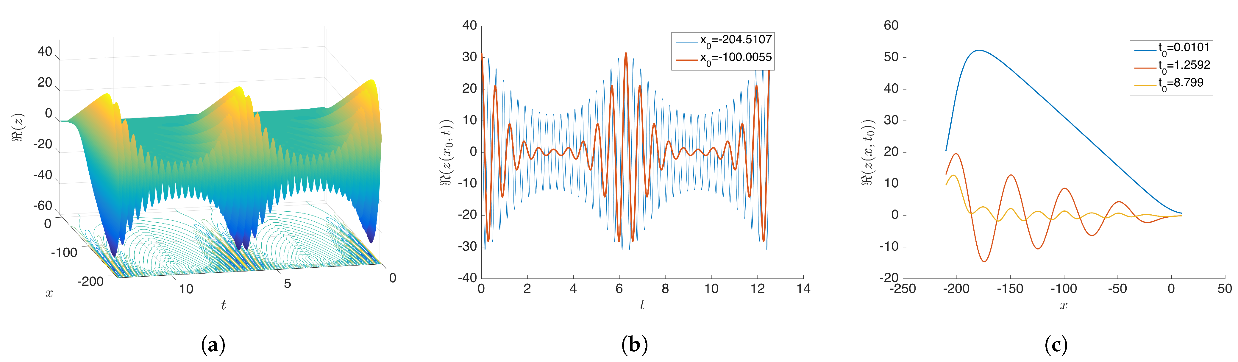
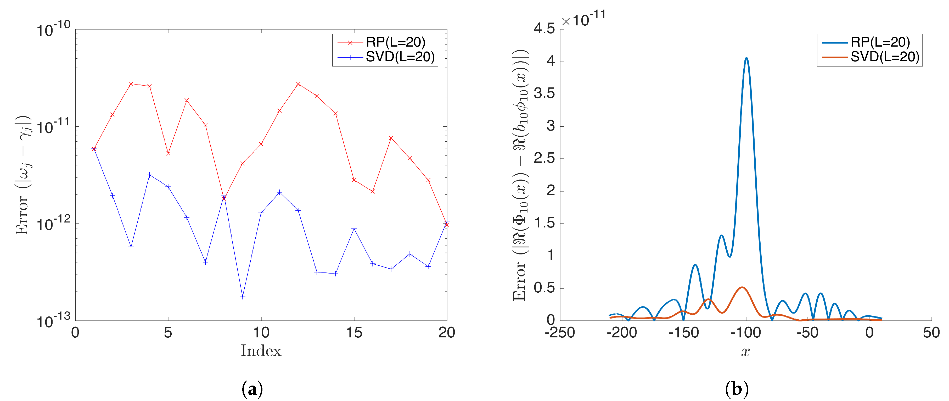
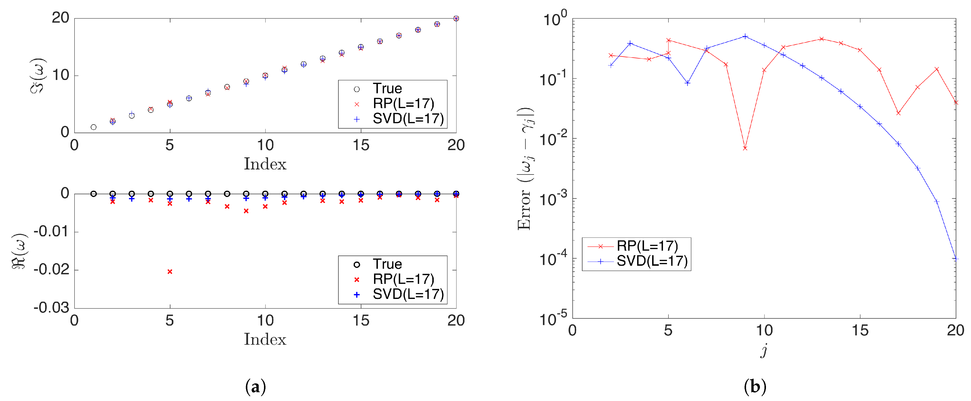
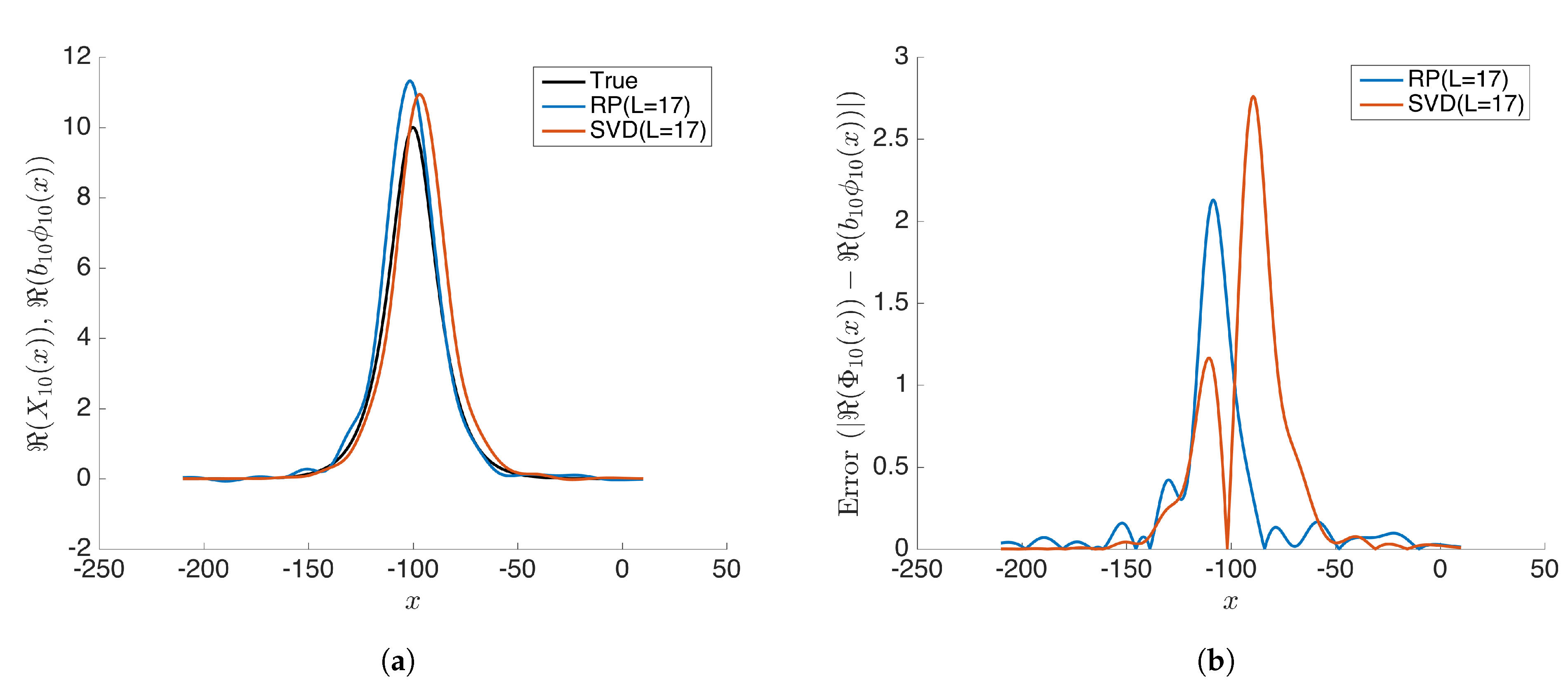
4.2. Toy Example: Demonstrates the Variable Separation and Isolating Dynamics

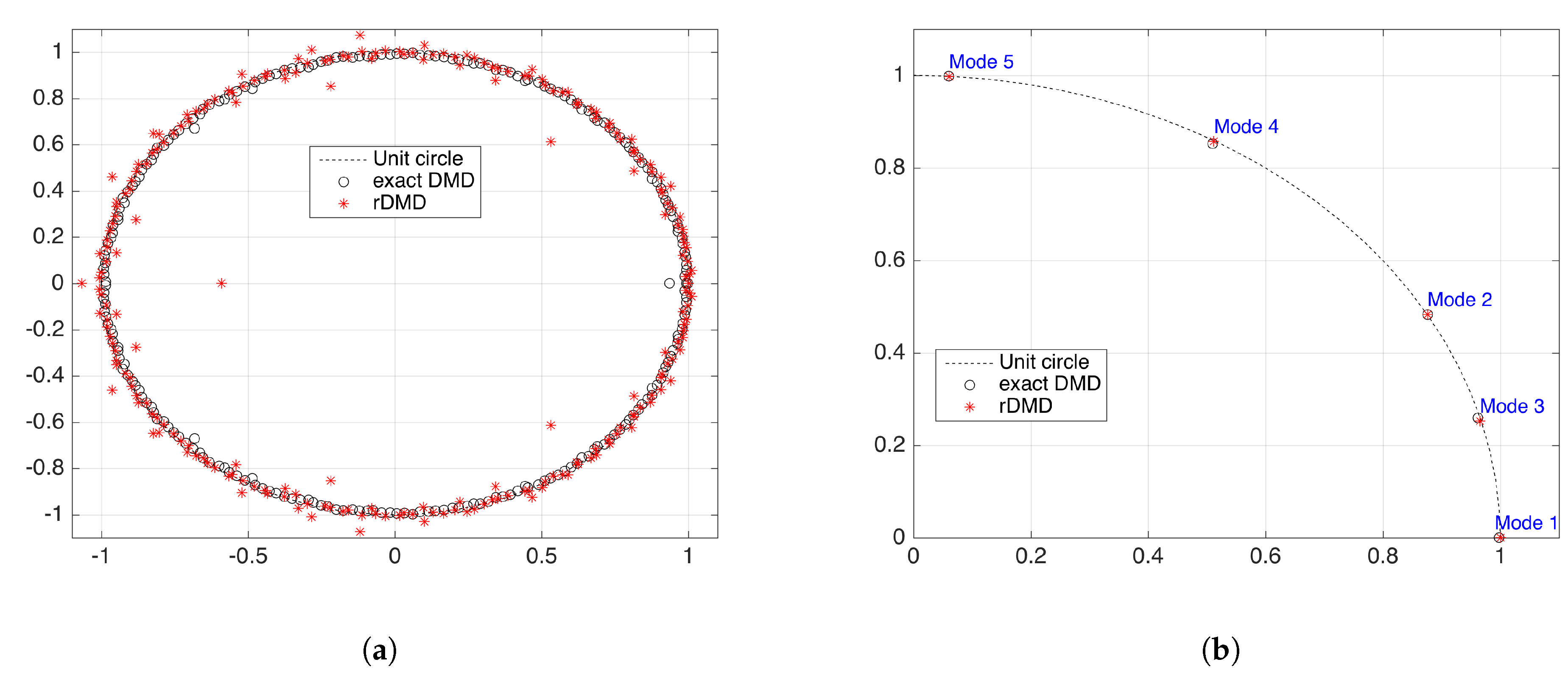
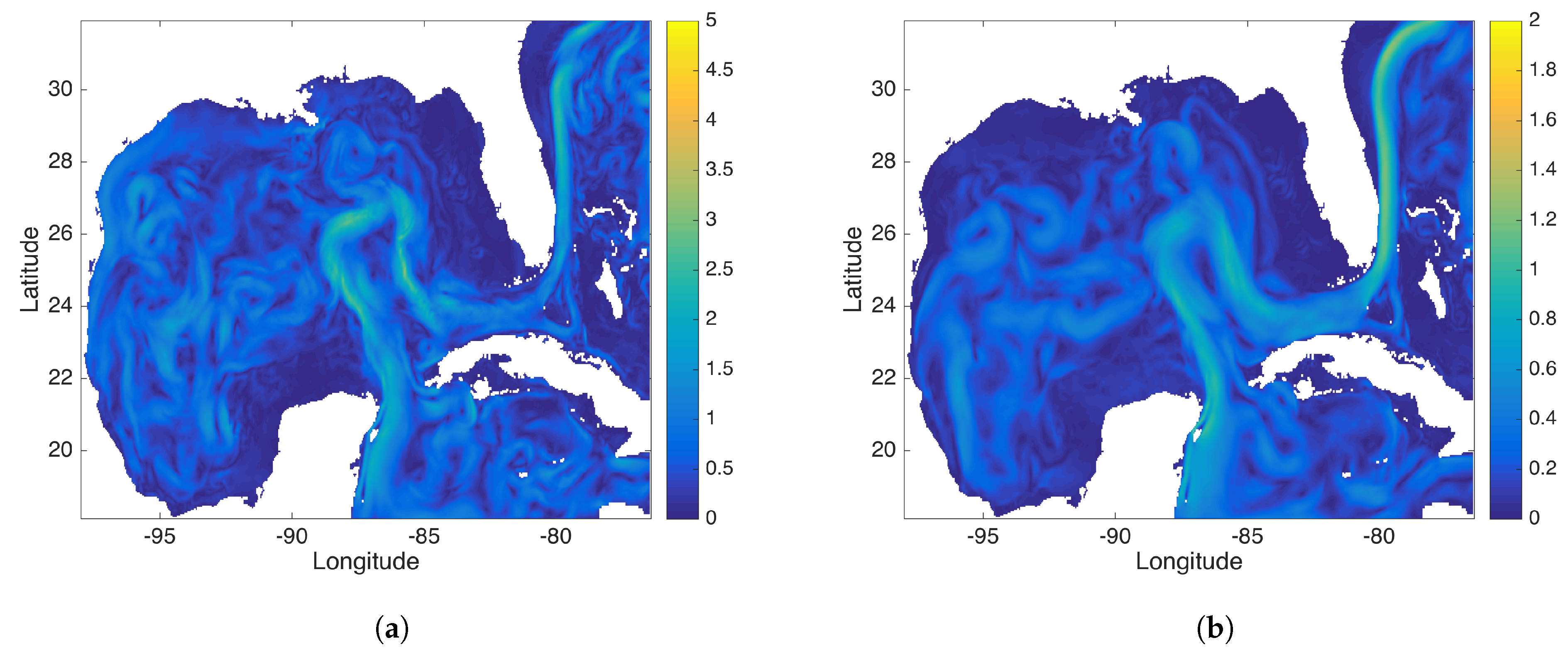
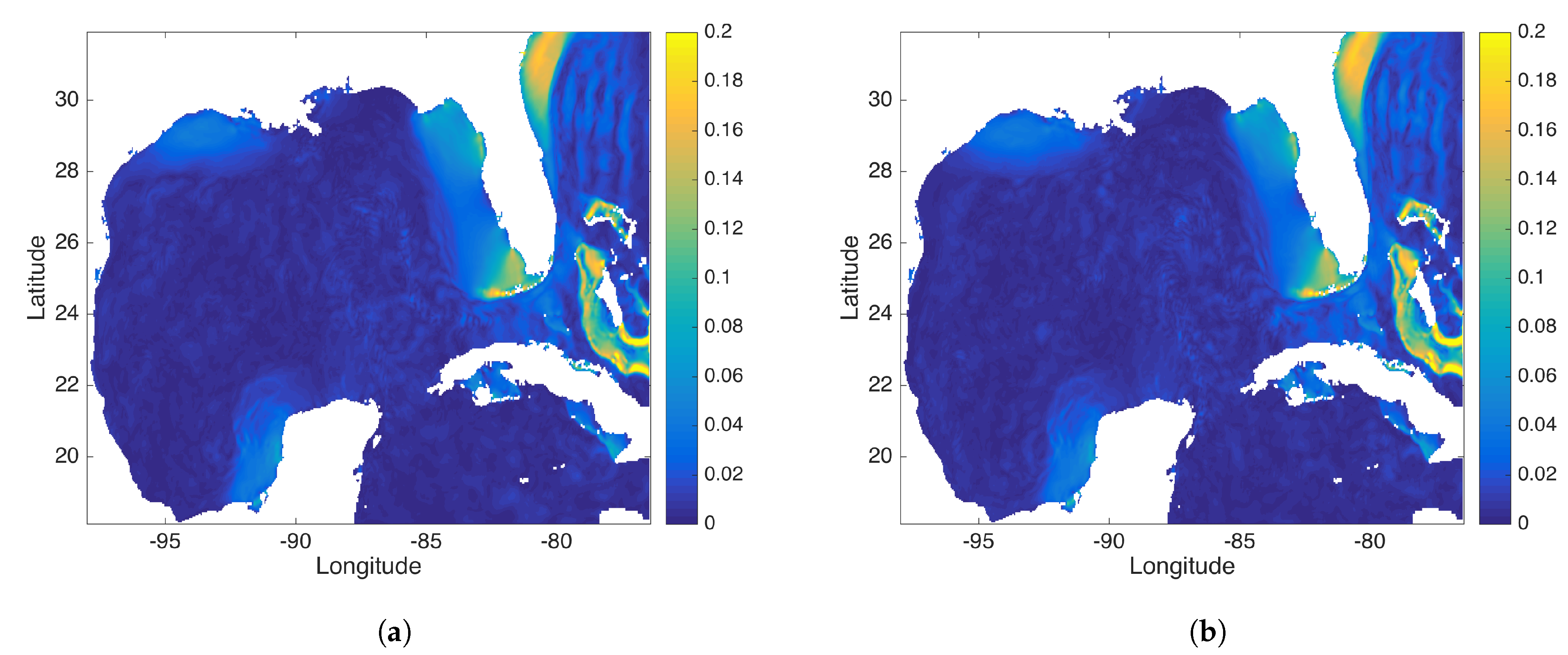
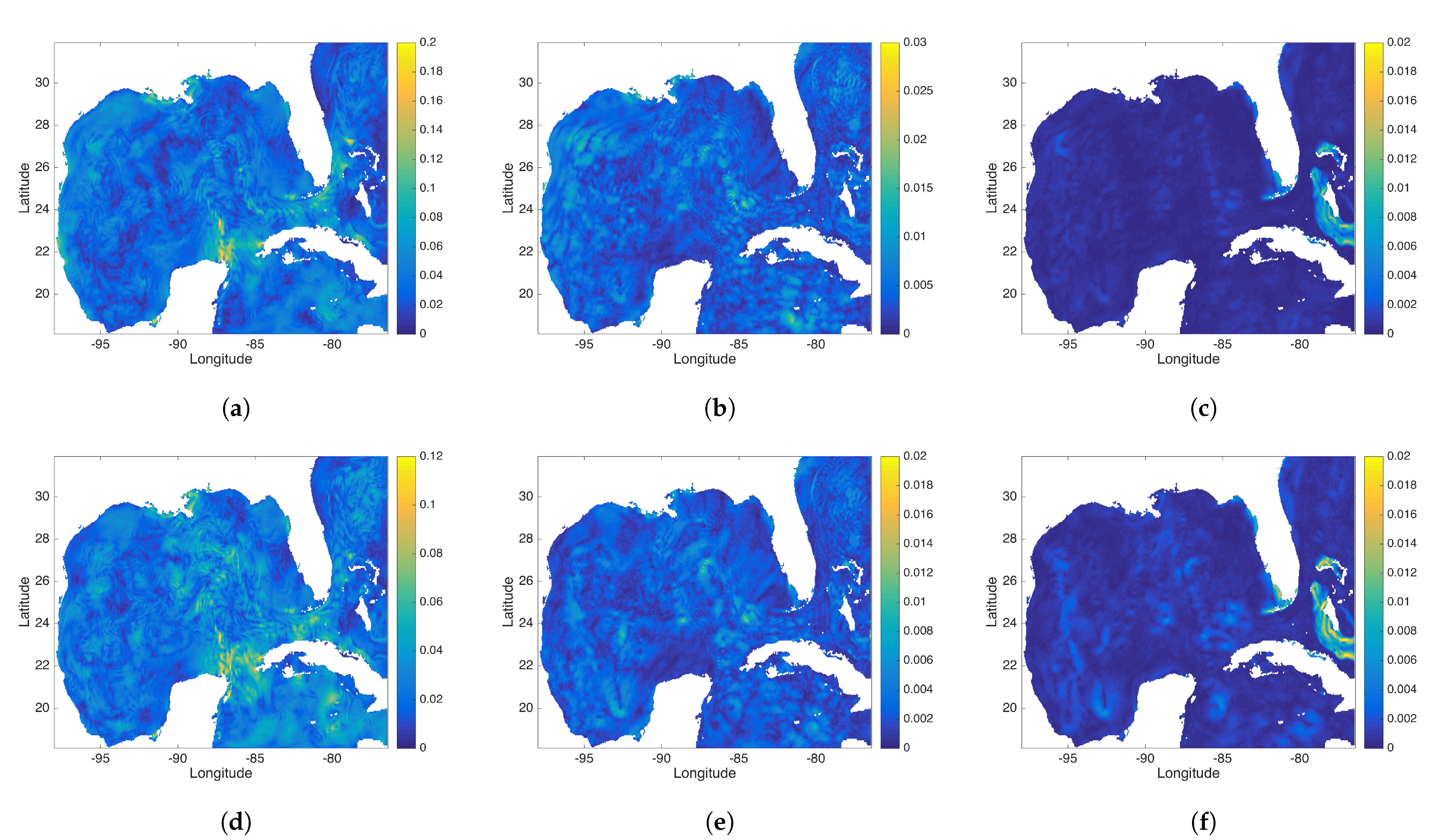
To demonstrate the variable separation and to isolate the spatial structures based on the time dynamics, we consider a toy example (motivated by [13]),

$$\begin{array}{c}\hfill z(x,t)=\sum _{j=1}^{20}j\mathrm{sech}(0.1x+j)e^{i{\gamma }_{j}t}=\sum _{j=1}^{20}{\Phi }_j\left(x\right)T_j\left(t\right)\end{array}$$

(15)

where ${\gamma }_j$’s are constants, and let ${\Phi }_j\left(x\right)=j\mathrm{sech}(0.1x+j)$ and $T_j\left(t\right)=e^{i{\gamma }_{j}t}$.

Comparing this Equation (15) with decomposition Equation (8), the rDMD algorithm is expected to isolate 20 periodic modes by rDMD algorithm. The data set (snapshot matrix) for this problem is constructed by $N=$ 20,000 spatial grid points and $M=5001$ temporal grid points with ${\gamma }_j=j$ (see Figure 7). As discussed in the previous section, if $L\ge 20$ then those expected modes can be isolated and there exist eigenvalues ${\lambda }_j$ of an rDMD operator, such that

$$\begin{array}{c}\hfill {\omega }_j=ln\left({\lambda }_j\right)=ji\end{array}$$

for $j=1,2,\cdots ,20$ (see Figure 8). Furthermore, we expect corresponding rDMD modes equal to spatial variables of the model, such that

$$\begin{array}{c}\hfill b_j\left(x_0\right){\varphi }_j\left(x\right)=j\mathrm{sech}(0.1x+j)={\Phi }_j\left(x\right).\end{array}$$

Figure 7. Original dataset constructed by Equation (15). (a) shows the $\mathrm{Re}\left(z\right(x,t\left)\right)$ plot for all $x,t$ values at 20,000 $\times 5000$ grid points. (b) represents the time series plot for two initial conditions. (c) provides the snapshots of few different time points. Our goal is separate and isolate spatial variables ${\Phi }_j\left(x\right)=j\mathrm{sech}(0.1x+j)$ and $T_j\left(t\right)=e^{ijt}$ from the given data constructed by $z(x,t)$.

Figure 8. (a) Shows the absolute error for estimated eigenvalues from rDMD and the exact DMD when the dimension of the projected space L = 20. (b) Shows the absolute error for the estimated 10th DMD mode by rDMD and exact DMD methods. In this case, both methods have very accurate results and error is less than ${10}^{-10}$.

As expected, we noticed that the calculated modes have negligible error when the dimension of projected space $L\ge r=20$. Figure 8 shows the absolute error of eigenvalues and DMD modes. All modes behave similarly; here, we present mode 10 for demonstration purposes by the SVD-based exact DMD method and the random projection based rDMD method. Notice that errors of both methods are less than ${10}^{-10}$ when $L\ge r=20$.

Further, we examine the case when the projected dimension $L=17<r=20$ and compare the results of rDMD with the exact DMD. We notice that both methods demonstrate similar errors and rDMD is almost as good as the SVD projection-based exact DMD (see Figure 9 and Figure 10). When the number of actual modes(r) is larger than the dimension of the projected space (L), the projected DMD operator only estimates the L number of modes, leading to both truncation errors and errors for eigenpair estimation based on the projected DMD operator. The $L<r$ case can be modeled as,

$$\begin{array}{c}\hfill z(x,t)=\sum _{j=1}^L{\widehat{b}}_j{\widehat{\varphi }}_j\left(x\right)e^{{\widehat{\omega }}_{j}it}+E_{L+1}\end{array}$$

(16)

where $E_{L+1}={\sum }_{L=j+1}^m{b}_j{\varphi }_j\left(x\right)e^{{\omega }_{j}it}$ is the truncated error that also affects the estimation process of eigenpairs. Therefore, if $L<r$, then there exists an error in eigenvalues and eigenvectors calculated by any method based on the projected DMD. However, this example demonstrates that rDMD can provide the results as good as the SVD projection-based method with very low computational costs (See Table 2).

Figure 9. (a) Compares the eigenvalues ${\omega }_j=ln{\lambda }_j$ calculated from rDMD (random projection(RP) with L = 17) and exact DMD (SVD projection with L = 17) methods with the expected true values ${\gamma }_j=ji$. Here, $L=17<20$ is the dimension of the projected space. (b) Shows the absolute error for the estimated eigenvalues from rDMD and exact DMD.

Figure 10. (a) Compares the modes $b_{10}{\varphi }_{10}\left(x\right)$ calculated from rDMD (random projection(RP) with L = 17) and exact DMD (SVD projection with L = 17) methods with the expected true values ${\Phi }_{10}\left(x\right)=10\mathrm{sech}(0.1x+10)$. (b) Shows the absolute error for estimated values from rDMD and exact DMD.

Table 2. Computational costs for the SVD-based exact DMD and random projection-based rDMD method for the data simulated by Equation (15). Computational costs of SVD for the high-dimensional snapshot matrix is relatively larger than random projection.

Method	Projected by	Computational Time (s)
Exact DMD	SVD	521.09
rDMD	Random Projection	2.35

4.3. Gulf of Mexico

In this example, we consider the data from HYbrid Coordinate Ocean Model (HYCOM) [14], which simulates the ocean data around the Gulf of Mexico. We used hourly surface velocity component ($u,v$) with $1/{25}^0$ spatial resolution ($N=541\times 347$ grid points) data for 10 days (240 $\mathrm{h}$ and $M=239$). Understanding the dynamics from the oceanographic data is an interesting application of DMD because those dynamics can be decomposed by tidal constituents. Hence, we are expected to isolate the dynamics associated with the tidal period; in other words, the final DMD mode selection is based on the period $P_i=2\pi /\mathrm{Im}(ln\left({\lambda }_i\right))$ of the modes(see Table 3). We constructed the snapshot matrix

$$\begin{array}{c}\hfill X=\left[\begin{array}{c}u\\ v\end{array}\right]\end{array}$$

(17)

by stacking the snapshots of velocity components ($u,v$) in each column to perform the DMD analysis.

Table 3. DMD modes for the Gulf of Mexico data set. Modes are selected based on the association to the tidal periods.

Mode	Period (h)		Associated Feature
	DMD	rDMD
1	∞	∞	Gulf stream around the GOM (see Figure 12)
2	$12.47$	$12.47$	Semi-diurnal tidal constituents (see Figure 13)
3	$23.85$	$24.56$	Diurnal tidal constituents (see Figure 14)
4	$6.08$	$6.07$	Second harmonic to semi-diurnal tidal constituents (see Figure 14)
5	$4.16$	$4.17$	Third harmonic to semi-diurnal tidal constituents (see Figure 14)

Figure 11 shows that most of the eigenvalues calculated from the SVD-based exact DMD and random projection-based rDMD are in agreement. Furthermore, eigenvalues that isolated the specific dynamics are almost equal. Additionally, Figure 12, Figure 13 and Figure 14 show the spacial profile of those modes from the exact DMD and rDMD methods. Moreover, each mode clearly isolate the interesting oceanographic features (see Table 3) and both methods provide almost the same spacial structures(see Figure 12, Figure 13 and Figure 14) as expected.

Figure 11. Eigenvalues ${\lambda }_i$ calculated from the exact DMD and rDMD methods. (a) Full spectrum of the two methods with projected space dimension L = 239 and (b) shows the first five modes. The mode selection is based on the comparison of the tidal periods with period of the DMD modes.

Figure 12. This figure compares the (a) DMD and (b) rDMD background mode identified by data from the Gulf of Mexico (GOM). This background mode captures the ocean current passing through the GOM.

Figure 13. This figure compares the (a) DMD and (b) rDMD mode associated with the M2 tidal frequency. This mode capture the “red tides”.

Figure 14. (a–c) represent the exact DMD modes 3, 4, and 5 and (d–f) show the rDMD modes 3, 4, and 5. Mode 3 is a diurnal mode with period $23.85$ h for the exact DMD case and $24.56$ h for the rDMD case. Modes 4 and 5 are associated with the second and third harmonic of semi-diurnal tidal constituents, respectively.

Notice that the dimension of the snapshot matrix is 375,454 × 239 and the SVD calculation of this matrix is more costly for both computation and storage. On the other hand, random projection only performs by the matrix multiplication, which could be done at a relatively low cost. Hence, we achieve almost the same results by using the random projection method, at relatively lower computational and storage costs.

5. Conclusions

We demonstrated that our rDMD can achieve very accurate results with low-dimensional data embedded in a high-dimensional observable space. Recent analytic technology from the concepts of high-dimensional geometry of data, and concentration of measure, have shown—surprising, if not initially intuitively—that even random projection methods can be quite powerful and capable. Here, in the setting of DMD methods approximating and projecting the action of a Koopman operator, we show that randomized projection can be developed and analyzed rigorously by the Johnson-Lindenstrauss theorem formalism, showing a powerful and simple approach. We provided a theoretical framework and experimental results to address those issues raised from SVD-based methods by introducing our new rDMD algorithm. The theoretical framework is based on generalizing the SVD-based concept as a projection of high-dimensional data into a low-dimensional space. We proved that eigenpairs of DMD in the original space can be estimated by using any rank L projection matrix P. Being able to estimate eigenpairs allowed us to use the powerful and simple Johnson–Lindenstrauss lemma and the random projection method, allowing us to project data with matrix multiplication. Therefore, our proposed random projection-based DMD (rDMD) can estimate eigenpairs of the DMD operator with low storage and computational costs. Further, the error of the estimation can be controlled by choosing the dimension of the projected space; we demonstrated this error bound through the “logistic map” example.

DMD promises the separation of the spatial and time variables from data. Hence, we experimentally demonstrated how well the rDMD algorithm performed this task by a toy example. Notice that the number of those isolated modes (m) are relatively (i.e., to spatial and temporal resolution) low in practical applications. If $m<<M$, then the rank of the data matrix is much lower, and those eigenvalues and vectors of interest can be estimated accurately by projecting data into the much lower dimensional space $L\ge m$. The SVD projection-based exact DMD method still needs to calculate the SVD of a high-dimensional (roughly ${10}^{10}\times {10}^3$ ) data matrix, while rDMD only requires multiplying the data matrix by a much lower-dimensional projection matrix. Furthermore, we noticed that both exact and random DMD methods experience similar errors. However random projection is much faster and needs less space for the calculations. We also demonstrate that practical applications provide similar results by using oceanographic data from the Gulf of Mexico.

Since the size of the DMD matrix is enormous in those applications (this could be roughly ${10}^{10}\times {10}^{10}$), the eigenpairs must be estimated by projecting data into the low-dimensional space. Estimating eigenvalues and eigenvectors of a DMD operator using a high-dimensional snapshot data matrix (in applications, this could be ${10}^{10}\times {10}^3$) with existing SVD-based methods is expensive. The computational efficiency of the rDMD led to a new path of the current Koopman analysis. It allows using more observable variables in the data matrix without need for much extra computational power. Hence, state variables and more non-linear terms can be used in an analysis, with low costs, to improve the Koopman modes. The JL theory can be adopted further into the field of numerical methods of the Koopman theory. As a next step, we can use the random projection concept in the extended DMD and kernel DMD methods.

References

- Schmid, P.J. Dynamic mode decomposition of numerical and experimental data. J. Fluid Mech. 2010, 656, 5–28. [Google Scholar] [CrossRef] [Green Version]
- Rowley, C.W.; Mezić, I.; Bagheri, S.; Schlatter, P.; Henningson, D.S. Spectral analysis of nonlinear flows. J. Fluid Mech. 2009, 641, 115–127. [Google Scholar] [CrossRef] [Green Version]
- Tu, J.H.; Rowley, C.W.; Luchtenburg, D.M.; Brunton, S.L.; Kutz, J.N. On dynamic mode decomposition: Theory and applications. J. Comput. Dyn. 2014, 1, 391–421. [Google Scholar] [CrossRef] [Green Version]
- Dasgupta, S. Experiments with Random Projection. In Proceedings of the 16th Conference on Uncertainty in Artificial Intelligence (UAI ’00), Stanford, CA, USA, 30 June–3 July 2000; Morgan Kaufmann Publishers Inc.: San Francisco, CA, USA, 2000; pp. 143–151. [Google Scholar]
- Johnson, W.B.; Lindenstrauss, J.; Schechtman, G. Extensions of lipschitz maps into Banach spaces. Isr. J. Math. 1986, 54, 129–138. [Google Scholar] [CrossRef]
- Bingham, E.; Mannila, H. Random Projection in Dimensionality Reduction: Applications to Image and Text Data. In Proceedings of the Seventh ACM SIGKDD International Conference on Knowledge Discovery and Data Mining (KDD ’01), San Francisco, CA, USA, 26–29 August 2001; Association for Computing Machinery: New York, NY, USA, 2001; pp. 245–250. [Google Scholar]
- Koopman, B.O. Hamiltonian Systems and Transformation in Hilbert Space. Proc. Natl. Acad. Sci. USA 1931, 17, 315–318. [Google Scholar] [CrossRef] [PubMed] [Green Version]
- Bollt, E.M. Geometric considerations of a good dictionary for Koopman analysis of dynamical systems: Cardinality, “primary eigenfunction,” and efficient representation. Commun. Nonlinear Sci. Numer. Simul. 2021, 100, 105833. [Google Scholar] [CrossRef]
- Chen, K.K.; Tu, J.H.; Rowley, C.W. Variants of Dynamic Mode Decomposition: Boundary Condition, Koopman, and Fourier Analyses. J. Nonlinear Sci. 2012, 22, 887–915. [Google Scholar]
- McQuarrie, S.A.; Huang, C.; Willcox, K.E. Data-driven reduced-order models via regularised Operator Inference for a single-injector combustion process. J. R. Soc. N. Z. 2021, 51, 194–211. [Google Scholar] [CrossRef]
- Pan, S.; Arnold-Medabalimi, N.; Duraisamy, K. Sparsity-promoting algorithms for the discovery of informative Koopman-invariant subspaces. J. Fluid Mech. 2021, 917. [Google Scholar] [CrossRef]
- Achlioptas, D. Database-friendly random projections: Johnson–Lindenstrauss with binary coins. J. Comput. Syst. Sci. 2003, 66, 671–687, Special Issue on PODS 2001. [Google Scholar] [CrossRef] [Green Version]
- Kutz, N.J.; Brunton, S.L.; Brunton, B.W.; Proctor, J.L. Dynamic Mode Decomposition: Data-Driven Modeling of Complex Systems; Society for Industrial and Applied Mathematics: Philadelphia, PA, USA, 2016. [Google Scholar]
- HYCOM + NCODA Gulf of Mexico 1/25° Analysis. 2021. Available online: https://www.hycom.org/data/gomu0pt04/expt-90pt1m000 (accessed on 28 October 2021).
Publisher’s Note: MDPI stays neutral with regard to jurisdictional claims in published maps and institutional affiliations. |
© 2021 by the authors. Licensee MDPI, Basel, Switzerland. This article is an open access article distributed under the terms and conditions of the Creative Commons Attribution (CC BY) license (https://creativecommons.org/licenses/by/4.0/).