Article

Deep Learning Approach to Mechanical Property Prediction of Single-Network Hydrogel

International Center for Applied Mechanics, State Key Laboratory for Strength and Vibration of Mechanical Structures, School of Aerospace Engineering, Xi’an Jiaotong University, Xi’an 710049, China
*
Author to whom correspondence should be addressed.
Mathematics 2021, 9(21), 2804; https://doi.org/10.3390/math9212804
Submission received: 30 September 2021 / Revised: 29 October 2021 / Accepted: 1 November 2021 / Published: 4 November 2021

Abstract

:
Hydrogel has a complex network structure with inhomogeneous and random distribution of polymer chains. Much effort has been paid to fully understand the relationship between mesoscopic network structure and macroscopic mechanical properties of hydrogels. In this paper, we develop a deep learning approach to predict the mechanical properties of hydrogels from polymer network structures. First, network structural models of hydrogels are constructed from mesoscopic scale using self-avoiding walk method. The constructed model is similar to the real hydrogel network. Then, two deep learning models are proposed to capture the nonlinear mapping from mesoscopic hydrogel network structural model to its macroscale mechanical property. A deep neural network and a 3D convolutional neural network containing the physical information of the network structural model are implemented to predict the nominal stress–stretch curves of hydrogels under uniaxial tension. Our results show that the end-to-end deep learning framework can effectively predict the nominal stress–stretch curves of hydrogel within a wide range of mesoscopic network structures, which demonstrates that the deep learning models are able to capture the internal relationship between complex network structures and mechanical properties. We hope this approach can provide guidance to structural design and material property design of different soft materials.

1. Introduction

With remarkable mechanical properties, hydrogels demonstrate high potential to be one of the advanced smart materials in the future [1,2]. Various superior properties of hydrogels have been discovered, such as high stretchability [3], biocompatibility [4], self-healing [5], and toughness [6]. On the basis of these properties, hydrogels are expected to pave the way for future applications such as drug delivery [7], flexible electronics [8,9], tissue engineering [10,11,12], and optical components [13,14,15]. Because the effect of polymer network structure on the mechanical properties of hydrogel is significant, a deeper understanding of polymer network can help us to better utilize the existed material and create new material. Therefore, it is imperative to investigate the relationship between the network structures and mechanical properties of hydrogels.
The mechanical properties of hydrogels are studied from different scales, from microscopic scale to continuum scale. The constitutive model constructed at the continuum scale is widely used and practical [16], however, some of them are lack of physical meanings and the parameters of the constitutive model are not universal to hydrogels with different ingredients proportion. It is because that the continuum scale model cannot reflect the real structure of hydrogel network. At the microscopic level, the mechanical properties of hydrogels are usually studied using molecular dynamics methods. However, it is difficult to overcome the issues of small size and time-consuming natures of the molecular dynamics simulations. The mesoscopic hydrogel model is expected to link the microscopic and the continuum scales and act as an important complement between them, providing a new theoretical framework for hydrogel research. Recent research on hydrogels at the mesoscopic scale is still in its infancy [17,18,19,20,21]. Obtaining valuable information from the mesoscale model can help to better understand the relationship between network structure and mechanical property. Proper hydrogel network models are in urgent need to essentially describe multiple mechanical behaviors of hydrogels. Therefore, we develop a generating method of mesoscopic hydrogel network based on self-avoiding walk (SAW) network model. There are several main advantages of mesoscopic hydrogel model, such as discrete systems, the characterization of complexity and stochasticity, and the reflection of mesoscopic structure of hydrogels. In fact, the complex physical relationship between the hydrogel network structure and its corresponding properties is often difficult to accurately express with current constitutive theories. In current studies on hydrogel mechanical property, results of phenomenological theory are not accurate enough, and numerical simulations are often time-consuming. In order to rapidly describe the mechanical properties of hydrogels, machine learning (ML) offers the benefit of extremely fast inference and requires only a basic dataset to learn the relationship between hydrogel network structure and mechanical properties.
With the development of ML, various ML algorithms have been widely applied to the field of engineering. Traditional ML algorithms have been used for data-driven solutions to mechanical problems [22,23,24,25]. There are also studies on the parameter determination of hydrogel constitutive model [26] and self-assembly hydrogel design [27]. In addition to using ML to establish implicit input-output relationships to solve regression problems, recently there is a new paradigm of physical informed neural network [28] that extends the learning capability of neural network (NN) to include physical equations and boundary conditions. Deep learning (DL) is a class of ML algorithms that uses multiple layers to progressively extract higher-level features from the raw input. DL has been successful in a wide range of applications, such as semantic segmentation, image classification, and face recognition [29,30,31,32]. The reason why DL significantly outperforms traditional ML is that the models are no longer limited to the multilayer perceptron (MLP) architecture, and are able to learn embedded and aggregated datasets. More specifically, DL methods provide a more advanced framework in which explicit feature engineering is not required and the trained model typically demonstrates higher generalization and robustness. Thereby, DL shows great potential in solving cross-scale prediction problems of structure–property relationship in the field of mechanics. Among the applications of DL algorithms in mechanics, it is proved that convolutional neural networks (CNNs) are significantly superior in damage identification and mechanical property prediction on composite materials [33,34,35,36,37]. In addition, Yang et al. [38] demonstrated how a deep residual network can be used to deduce the dislocation characteristics of a sample using only its surface strain profiles at small deformations for crystal plasticity prediction. Pandey and Pokharel [39] presented a DL modeling method to predict spatially resolved 3D crystal orientation evolution of polycrystalline materials under uniaxial tensile loading. Herriott and Spear [40] investigated the ability of deep learning models to predict microstructure-sensitive mechanical properties in metal additive manufacturing and Choi et al. [41] used artificial intelligence-based methods to investigate the fatigue life of the hyperelastic anisotropic elastomer W-CR material.
The advantages of CNNs for image-like data are mainly in the following aspects: firstly, by employing the concepts of receptive fields in the convolutional layer, CNNs could be a powerful tool for pattern recognition in computational mechanics and material problems that are characterized by local structural interactions [42]. Secondly, CNNs are able to effectively learn a certain representation of underlying symmetry and tend to be invariant to general affine input transformations such as translations, rotations, and small distortions [42]. These properties enable CNNs to characterize structures with heterogeneous and randomness, for instance, hydrogel network at the mesoscopic scale. Meanwhile, mesoscopic scale modeling studies often yield a large amount of high-dimensional data with corresponding physical information, which can be used to establish a modular and efficient mechanical modeling framework. However, there is still lack of using DL methods to study the mechanical properties of soft materials.
In this paper, we utilize deep neural network (DNN) and 3D CNN to reveal the implicit relationship between network structure and mechanical property of hydrogel, so as to predict mechanical property from different network structures. First, we propose a modeling method for single-network hydrogel network, that is, a self-avoiding walk network model, which approximates the real polyacrylamide (PAAm) hydrogel structure at a mesoscopic scale. Then, we develop a DNN based on MLP and a 3D CNN containing the physical information of the network, and use them to predict the nominal stress–stretch curves of hydrogels under uniaxial tension, because the stress–stretch relationship is one of the most important mechanical description that can be used to derive typical properties, such as modulus, toughness, and strength. Using a dataset of 2200 randomly generated network structures of PAAm hydrogel and their corresponding stress–stretch curves, we train and evaluate the performance of the two models. Based on the results of the error analysis and the performance of the two models on the training data, we compare and summarize their generalization capability.
The paper is organized as follows: in Section 2 we present the derivation of the constitutive model for PAAm hydrogel, the modeling method of hydrogel networks, and the basic knowledge of DNN and CNN algorithms. The modeling framework and architecture of the two DL models we developed are detailed in Section 3. Analysis and evaluation of the results for mechanical property prediction of hydrogel are demonstrated in Section 4. Finally, concluding remarks are provided in Section 5.

2. Methodology

2.1. Derivation of the Constitutive Model of Hydrogel

For effectively using hydrogel in engineering applications, it is very imperative to understand the mechanical properties of hydrogels. Although polymer physics and continuum mechanics provide a way to study the mechanical properties of hydrogels, uniaxial loading test is still a common method to test the mechanical property of hydrogel materials. In order to accurately predict the nominal stress–stretch relationship of hydrogel using DL method, a dataset of stress–stretch curves is needed for the model training. However, obtaining stress–stretch curves from experiment tests requires a lot of labor work, especially considering different polymer fractions of hydrogel. In this study, the relationship of stress and stretch is derived from the constitutive model we have proposed, which is used as the ground truth (prediction target) for DL model training.
In this study, to determine the relationship of stress and stretch whether from testing or theoretical prediction, the deformation process of hydrogel is divided into two steps: swelling process and loading process. During swelling process, because of the hydrophilia of polymer chains, the dry polymer can imbibe a large quantity of solvent and swell into hydrogel. The volume of hydrogel is the sum of absorbed solvent and dry polymer due to the law of conservation of mass. The hydrogel is assumed to be traction-free and reaches an equilibrium state at the end of the process, which represents the chemical potential is the same throughout the whole hydrogel and the external solvent. In the loading process, both ends of the dumbbell-shaped specimen are clamped. One end is held fixed on the foundation of the tensile testing machine and the other end is stretched with the elongation of the moveable clamp. The middle part of dumbbell-shaped specimen is under uniaxial tension state since two directions that are perpendicular to the loading direction are traction-free. At this state, hydrogel is no longer contacted with solvent and mechanical boundary condition is applied.
To derive the stress–stretch relationship of hydrogel during uniaxial loading, we adopt well-known free energy function due to Flory and Rehner [43,44]:
W = 1 2 N k T F i K F i K 3 2 log det F k T ν ν C log 1 + 1 ν C + χ 1 + ν C
where W is the free energy pure reference volume, N is the number of polymeric chains per reference volume, k is the Boltzmann constant, T is the absolute temperature, F is the deformation gradient of the current state related to the dry state, C is the concentration of solvent in the gel, ν is the volume per solvent molecule, and χ is a dimensionless parameter measuring the enthalpy of mixing. The reference state is chosen as the dry state before the polymer absorbs any solvent.
During the swelling process, all molecules in the gel are assumed to be incompressible. Therefore, the volume of the gel is the sum of the volume of the dry network and the volume of solvent:
1 + ν C = det   F
Using Legendre transformation, the free energy density function W F , C can be transformed into W ^ = W F , C μ C , which is the function of chemical potential μ and deformation gradient F . Considering the incompressible condition, the new free energy density function can be written as:
W ^ F , μ = 1 2 N k T I 3 2 log J k T ν J 1 log J J 1 + χ J μ ν J 1
where I = F i K F i K and J = det F .
Based on the assumption of two steps during the deformation process, the deformation gradient tensor F can be decomposed as F = F 0 F . F 0 is the deformation gradient of the free-swelling state related to the dry state. F is the deformation gradient of the mechanical loading state related to the free-swelling state. For a free-swelling process, when hydrogel reaches the equilibrium, F 0 = λ 0 I .
Since we prefer to use the free-swelling state as the reference state during mechanical test, the free energy density function with free-swelling state as the reference state is W ^ F , μ = λ 0 3 W ^ F , μ , which can be expanded as:
W ^ F , μ = λ 0 3 2 N k T λ 0 2 I 3 2 log λ 0 3 J k T v J λ 0 3 log J λ 0 3 J 1 + χ λ 0 6 J μ v J λ 0 3
where I = F i K F i K and J = det F . Because the volume is incompressible during the loading process, J equals to one and stretch λ 0 is a constant. With free-swelling state as the reference state, the free energy density function can be written as:
W ^ F , μ = λ 0 1 2 N k T I + A
where A is a constant given as:
A = λ 0 3 2 N k T 3 + 2 log λ 0 3 k T v 1 λ 0 3 log 1 λ 0 3 1 + χ λ 0 6 μ v 1 λ 0 3
During loading process, considering the volume incompressibility condition, we add a term p 1 det F to the free energy function W ^ F , μ , where p is a Lagrange multiplier, which can be determined by boundary conditions. Then the nominal stress can be calculated by:
s i k = W ^ F , μ + p 1 det F F i k
and we obtain the expression of nominal stress with free-swelling state as the reference state:
s i k = λ 0 1 N k T F i k p F i k T
For a uniaxial loading process, the deformation gradient tensor F is:
F = λ s 1 λ s 1 λ s
where λ s is the stretch along the uniaxial direction. The nominal stress along with and perpendicular to the uniaxial direction is s 1 , s 2 and s 3 , respectively. As the surface perpendicular to the uniaxial direction is traction-free, therefore, the expressions of nominal stress s 1 , s 2 and s 3 are as follows
s 1 = λ 0 1 N k T λ s p λ s 1 2
s 2 = s 3 = λ 0 1 N k T λ s 1 p λ s 1 2 = 0
The Lagrange multiplier is solved from Equation (11), and p = λ 0 1 N k T λ s 3 2 . The nominal stress along with the uniaxial direction is derived as:
s 1 = λ 0 1 N k T λ s λ s 2
We define the volume fraction of the polymer in the hydrogel as ϕ V , ϕ V = 1 J = 1 λ 0 3 . Under uniaxial loading, the nominal stress with free-swelling state as reference state is given as:
s 1 = ϕ V 1 3 N k T λ s λ s 2
After obtaining Equation (13), the nominal stress–stretch curves with different polymer fractions could be calculated. This equation reveals the relationship between mechanical response and material property of single-network hydrogel and can be used as the dataset for DL-based model training.

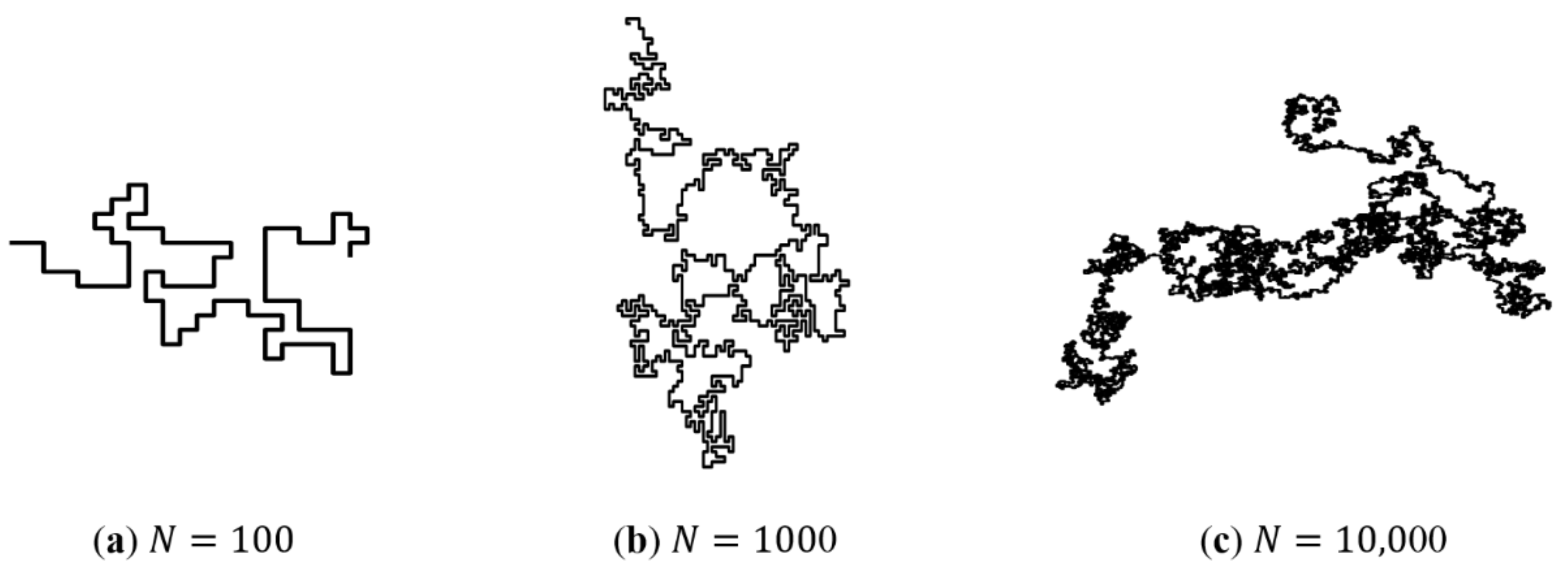
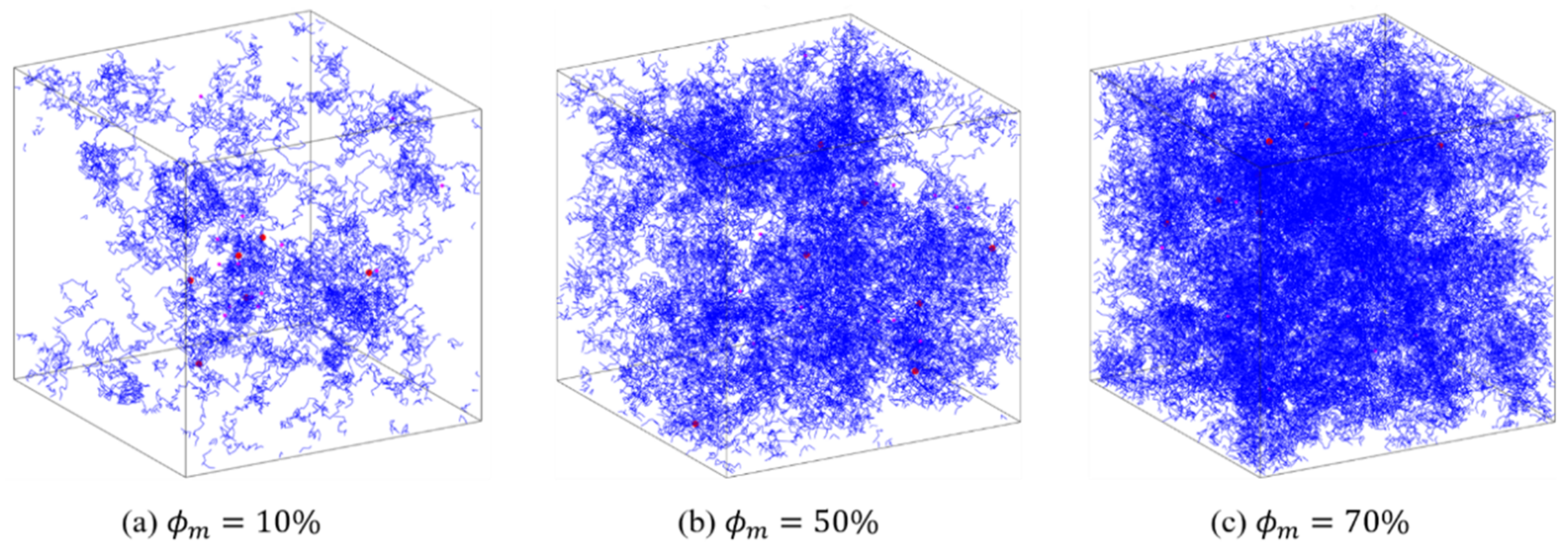
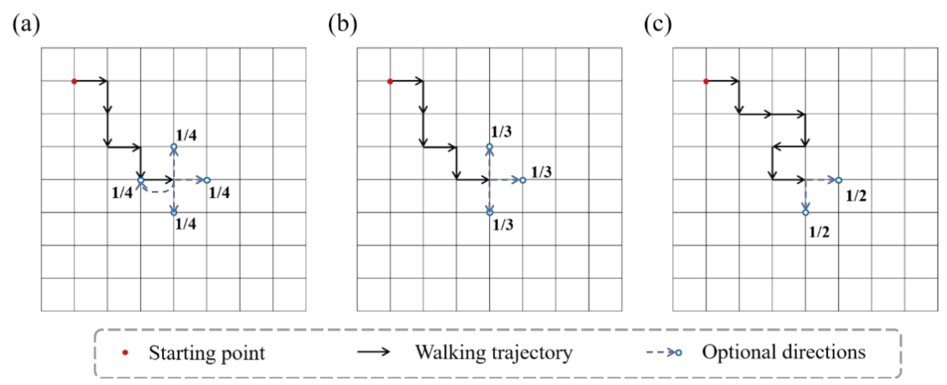
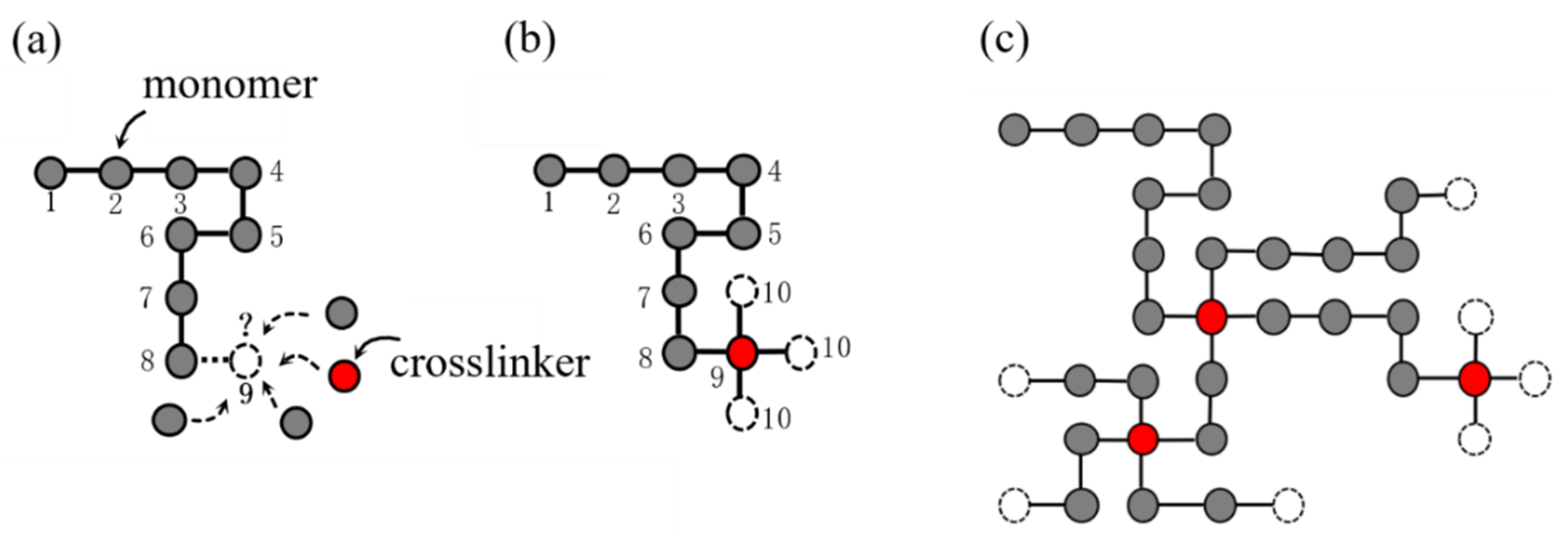
2.2. Network Generation Model of Single-Network Hydrogel

At mesoscopic scale, the hydrogels can be abstracted as polymer chains comprised by a large number of points and bond vectors [45,46]. Models at the mesoscopic scale can help us extract the commonalities of polymer chains, and make the research focus on the responses of structural changes of the chain and network, rather than the specific molecular properties at the microscopic scale or the complex boundary problems at the continuum scale. In order to describe the network configuration of single-network hydrogels at a mesoscopic scale, we develop a mathematical model using SAW to characterize the randomness, uniqueness, and heterogeneity of polymer chains. In addition, the model potentially reproduces a configuration that is statistically similar to the true structure of polymer chains.
The configuration of molecular chains of single-network hydrogels can be abstracted as bond vectors connected end to end, which is geometrically similar to a walking trajectory in space. Random walk (RW) is a mathematical model describing a random process in the lattice space. RW describes a series of random steps starting from a point in a discrete lattice space. An example of RW in two-dimensional space is shown in Figure 1a. Assuming that the end of the chain is the ongoing random walk, then the next step is to choose from up, down, left, and right directions (including the direction to the point of the previous step). The probability of each direction is 1/4. After selecting the next direction, the chain takes one step to the neighboring node, then randomly selects a direction again for the next step, and so on. The RW model allows the walking trajectory to repeatedly visit the same node. Besides, the SAW model is also a commonly used mathematical model to describe the configuration of polymers. The SAW model is derived from the RW model. The main difference between the two models is that the SAW model does not allow the walking trajectory to visit the same point repeatedly. Because the SAW model does not allow to go back, each node has at most three alternative directions in two-dimensional space, as shown in Figure 1b. If some of the three directions have been previously visited by this chain or other chains in the same space, the SAW model will not select this direction at the next step, as shown in Figure 1c.
Figure 2 shows the SAW trajectory with different number of steps N . It can be seen that with N increase, the configuration of the SAW trajectory is geometrically similar to the configuration of the real polymer chain.
The SAW model is able to generate one long chain, but not multiple paths. In order to generate a complex network model reflecting the configuration of the hydrogel network, we propose a SAW-based network generation algorithm (NGA). Because polyacrylamide (PAAm) hydrogel basically does not conduct viscoelasticity or damage accumulation effect during the loading process, and it can be described as nearly elastic using hyperelastic constitutive model to its mechanical properties, we take the PAAm hydrogel as an example. The design ideas of the NGA are quite similar to the actual generation process of hydrogel network. Figure 3 shows the design logic of the NGA. Take two-dimensional space as an example, consider that each point in the discrete space can only be occupied by one particle, that is, one from monomer particles (gray dots), crosslinker particles (red dots), or water molecules (void space). Before the NGA starts, it is necessary to set the space size w , the number of monomer particles n m o n and the number of crosslinker particles n c r o , so that the polymer volume fraction of the network can be determined as:
ϕ V = n m o n + n c r o w 3 n m o n w 3
where considering n m o n n c r o , Equation (14) gives the polymer volume fraction in the NGA. While the NGA is running, a SAW starts to wander from the original point in the space. Each step of the SAW represents a certain type of particle assembled into the chain and becomes part of the chain. In each step of the SAW, the probability of what kind of particles to be inserted depends on the number of remaining monomers and crosslinkers, as shown in Figure 3a. Each particle that has not been inserted has the same probability to be the next spatial point. Because one crosslinker of the PAAm hydrogels can link four monomers, if the nineth position is connected to the crosslinker, the tenth position will be branched out to form three new chain ends, as shown in Figure 3b. The SAW will continue on the basis of these three new chains. There is only one SAW chain at the beginning, then it will gradually bifurcate, and finally form a network structure, as shown in Figure 3c. In this study, this network model is called SAW network model, which is able to characterize the complex polymer network configuration of single-network hydrogels.
Since the space size w is limited, the SAW network generated by the NGA will eventually reach the boundary of the space. Therefore, we adopt periodic boundary conditions in this model. When the SAW touches the periodic boundary of the space, it will stop right there and no longer connect to any other particles. Instead, the periodic boundary condition makes it place a new chain starting point at the corresponding position on the other side of the space (a symmetrical position) and the SAW continues. This process is similar to a SAW path that goes out from one side of the space and enters from the other side of the space at the same time.
The examples above in 2D space are to make the design logic of the NGA easy to be understood. For the real configuration of hydrogel network, the NGA should be implemented in 3D space. In 3D space, each spatial point has 26 neighbors (including six surface neighbors, twelve side neighbors, and eight corner neighbors). Although the distances from the 26 neighbors to the center point are not all equal, when the size of these 27 local points compares with the size of the entire model space, the distance difference between neighbors is negligible.
In practical experiment, polymer mass fraction ϕ m is used as usual to measure the water content of hydrogels due to the ease of measuring the sample mass. For practical application of the NGA, polymer mass fraction ϕ m is adopted in the algorithm. The conversion relationship between polymer volume fraction ϕ V and polymer mass fraction ϕ m is given by:
ϕ m = 1 ϕ V 1 1 M w M m o n + 1
where M w is the molar mass of water. M m o n is the molar mass of AAm monomers. They are equal to M w = 18   g / mol and M m o n = 71.08   g / mol , respectively.
For the complex network of PAAm hydrogel, the SAW network model generated by the NGA in 3D space is shown in Figure 4. The different values of the model determined by n m o n , n c r o and w result in different polymer mass fractions ϕ m . In Figure 4, the blue lines represent polymer chains, and the red dots represent crosslinkers. When ϕ m is low, the distribution of polymer chains in the space is sparse and inhomogeneous. This proves the structural randomness, heterogeneity, and uniqueness of the polymer network of PAAm hydrogel. With the increase of ϕ m , the PAAm hydrogel network becomes gradually dense and is closer to the homogeneous assumption in continuum mechanics. Thus, this model has the potential in characterizing the mesoscopic configuration of single-network hydrogels and provides a powerful tool for follow-up research.

2.3. Deep Learning Algorithms and Approaches

Machine learning systems can be classified according to the amount and type of supervision they receive during training. There are four major categories: supervised, unsupervised, semi-supervised, and reinforcement learning. In the case of supervised learning, the input data set (containing samples and corresponding features) and labels (the correct results) are both necessary for training. On the contrary, unsupervised learning, as the name suggests, only provides unlabeled training data. For engineering problems, most of the applied ML algorithms are supervised learning with the datasets collected from experiments or simulations [47,48,49]. Artificial neural network (ANN) [50] is comprised of multiple interconnected computational elements called neurons. In this study, the algorithms we adopt belong to a subset of ANN. By adjusting parameters, for instance, weights and biases in a NN architecture, the algorithms we used can predict the mechanical property of hydrogel through an optimization of errors. Both the fully connected MLP and CNN belong to the class of ANN, and they differ primarily in their architecture and interconnectivity. This section gives a brief introduction to the main ML algorithms used in this work.

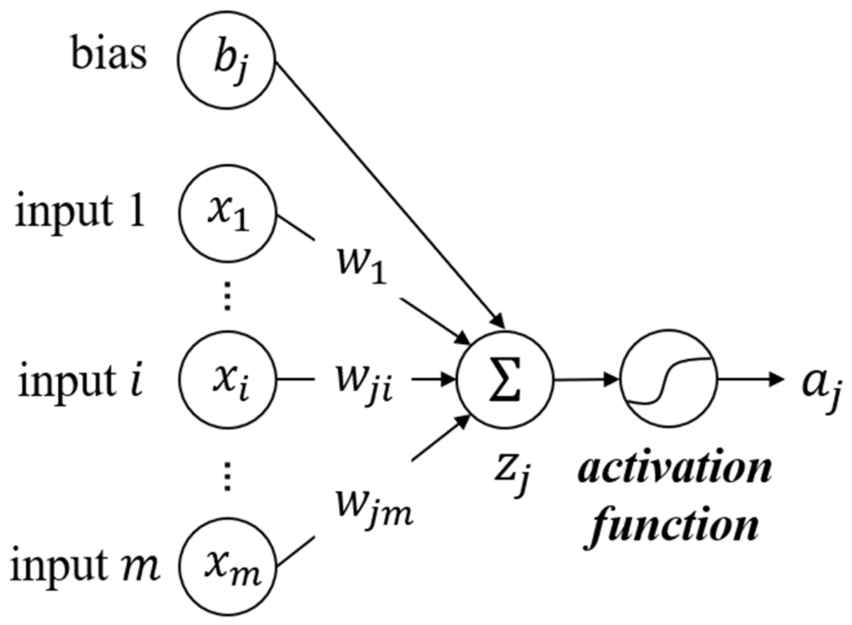
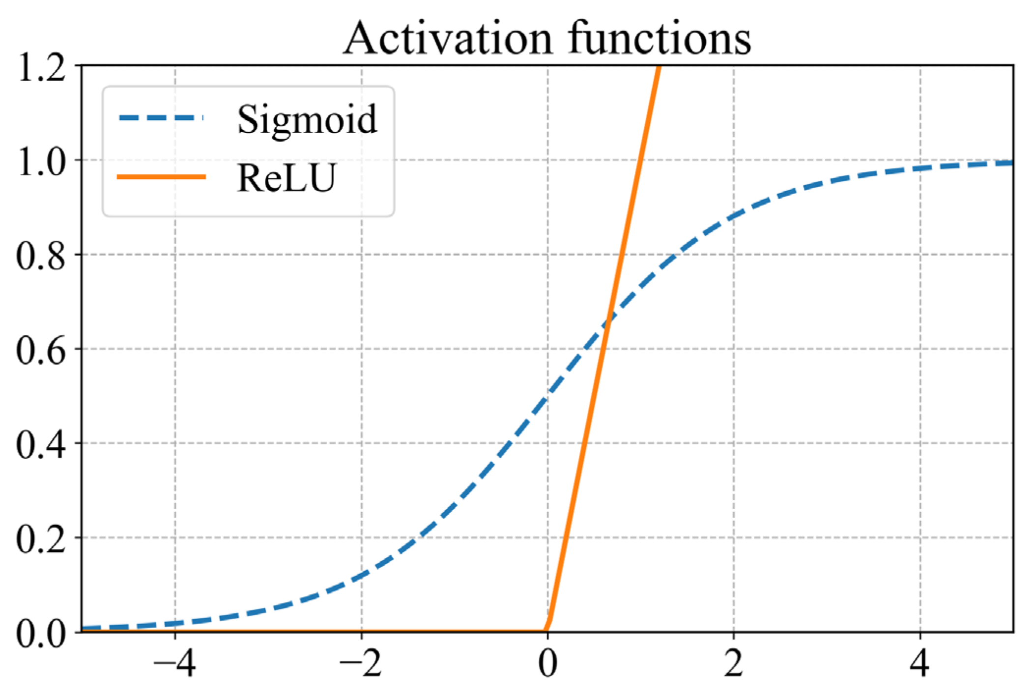
2.3.1. Multilayer Perceptron

The MLP architecture, generally called feedforward NN, is one of the most popular and widely used ML architectures that was proposed initially as a function approximator [51]. The aim of a MLP is to approximate a function f between input x and output y ^
y ^ = f x
In order to approximate strongly non-linear functional relations, MLP adds an additional level of hierarchy to linear learning algorithms involving features and learned weights by combining activation functions:
a j = σ z j = σ i = 1 m w j i x i + b j
where i denotes the i th neuron in the previous layer, and j the j th neuron in the current layer. a j is the output value of the current neuron. σ · is the activation function that usually takes a non-linear function. x i represents one feature input of x . w j i and b j are parameters updated during the training, named weight and bias, respectively. m is the number of neurons in the previous layer. z j is the sum of the input values and the bias, also the prediction of the linear learning model. This process is demonstrated in Figure 5, which is the typical mathematical process of a single neuron. Furthermore, matrix form can be written as:
a W , b X = σ X W + b
where X represents the matrix of input features. It has one row per sample and one column per feature. The weight matrix W contains all the connection weights, which has one row per input neuron in the previous layer and one column per artificial neuron in the current layer. b is the bias vector that has one bias term per artificial neuron. The weights of the MLP are usually initialized stochastically, and then subsequently tuned during the training. One way to train the MLP is to establish a linkage of its known input–output data and to minimize its loss function from the output by appropriately changing the weights.
There are several alternatives to the activation functions. Frequently used activation functions in regression tasks include the sigmoid function (Equation (19)) for the outputs required between the domain (0,1) and the rectified linear unit (ReLU) as shown in Equation (20) for nonzero outputs. The two functions are illustrated in Figure 6.
s i g m o i d z = 1 1 + e z
R e L U z = max 0 , z
It is the nonlinear transformation of the activation function that gives the MLP a strong nonlinear fitting capability. It should be noted that a feedforward NN can approximate any continuous functions with arbitrary complexity in the reach of arbitrary precision, using only one hidden layer containing enough neurons [52]. MLP is served as the beginning of research on more complex DL algorithms. Deep architecture has better learning capability by stacking more layers to extend the depth of the NN.

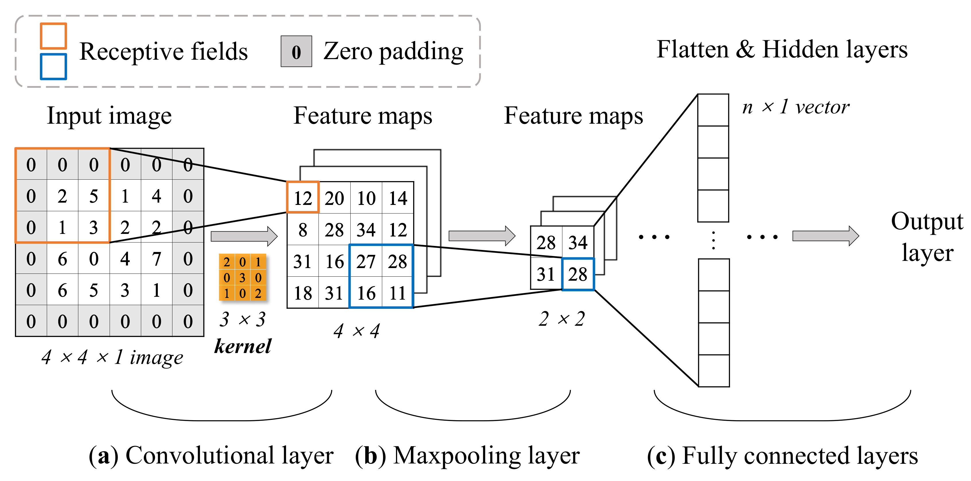
2.3.2. Convolutional Neural Network

Convolutional neural network is one of the most widely-used deep neural networks that is inspired by the study of the brain’s visual cortex, and CNN is extremely successful in the image recognition field. It has been extended to various applications of many other disciplines including mechanics.
There are two main differences between a fully connected MLP and a CNN, i.e., the input data structure and data transfer. Input data in a CNN is assumed to be an image or can be physically interpreted as an image. The input image contains many pixels and is a 2D data structure with length and width. Of course, the image can also be a 3D structure with three dimensions of length, width, and thickness. The 3D CNN model used in this study utilizes three3Dimensional data. Instead, in the case of the MLP, the inputs to the neurons in the hidden layer are obtained by a standard matrix multiplication X W of the weight W and the input X . Besides, in the case of the data transfer, MLP only feedforwards the input data obeying Equation (18). However, for CNNs, the input data will be transformed through a convolutional kernel (or called a filter) into a feature map using a convolution operation. This process is symbolically written as X W ( symbol represents convolution operation).
A typical CNN architecture is mainly comprised of four building blocks, and they are referred to as convolutional layers, pooling layers, fully connected layers, and activation functions. Take a 2D input image as an example:
It can be seen from Figure 7 that different layers have their corresponding functions. The convolutional layer is the core of a CNN model, each convolutional layer has one or several convolutional kernels (or filters). The kernels extract the features of the input image by scanning pixels (like a camera) in a small rectangle (called receptive field) using convolution operations, and repeat until the entire image is scanned. The shift from one receptive field to the next is called the stride. By default, stride equals one for convolutional layers and two for pooling layers. Indeed, a convolutional layer can contain multiple kernels (filters) and output one feature map per kernel. New feature maps (the number of newly generated feature maps depends on the number of filters in the convolutional layer) are generated with smaller height and width compared to the previous image. One pixel is one neuron in each feature map, and all neurons in the same feature map share the same parameters (the same weights and bias). In order to ensure each input image for a layer have the same height and width as the previous layer, it is common to add zeros around the inputs (zero padding), as shown in Figure 7a. Neurons in the first convolutional layer are not connected to every single pixel but only to pixels in the corresponding receptive fields. The role of the kernel allows features to be mapped through local interactions. This architecture allows the network only to focus on small low-level features in the first layer, then with more convolution layers repeating this feature extraction process, larger high-level features are assembled, and so on. That is why CNN is more effective than MLP on the input–output relationship learning of structures depending on spatial locations.
After the pre-activated convolutional operation, results are offset by a bias (one bias per convolutional layer). Then the feature maps are passed through nonlinear activation functions commonly referred to as ReLU. ReLU has been proven [52] to provide high computational efficiency and often achieves sufficient accuracy and performance in practice.
The max-pooling layer is usually implemented after one or multiple convolutional layers, making a key role in reducing the number of parameters thus resulting in a faster training process. Its goal is to subsample the input image for reducing the computational load by reducing the number of parameters and preventing the risk of overfitting. On the contrary to the convolution layer, a pooling neuron has no weights or bias, all it does is aggregate the inputs using an aggregate method, such as max or mean. Figure 7b simply shows how the max-pooling layer works. Subsequently, there is usually a fully connected layer at the end, which is no different from a typical MLP architecture at most times.
CNNs explain the topological structure of the input data, that is, allow stacking neural layers to extract high-level features. Actually, this hierarchical architecture is common in real images, which is one of the structural reasons why CNNs work so well on image recognition. Through the optimization process, the CNN model “learns” how the spatial arrangement of specific features are related to the outputs. Once trained, the CNN model can be used to make predictions with high computational efficiency. Compared with general projects in the DL field, the requirement of the number of datasets and features used in mechanical property prediction of hydrogels is much less. Therefore, the framework of the DL-based models employed in this study could be adjusted easily, and the increasing number of weights and biases has an acceptable impact on the computational cost. For this reason, DNN and CNN are finally used in this study to predict the macroscopic mechanical properties of hydrogel.

3. Deep Learning Modeling Framework for Single-Network Hydrogel

In this section, in order to explore the application potential of the SAW network model and the performance of the 3D CNN model in predicting the mechanical properties of hydrogels with complex network structures, we firstly design two types of data structures extracting structure–property linkages of hydrogels. Furthermore, we implement two deep learning models that are used to make predictions. For both models, the data samples are generated based on the SAW network model. The two datasets include training, validation, and testing sets, which reflect the ground truth. In this study, it should be noted that the labels are the nominal stress–stretch response of the single-network hydrogels under uniaxial tension, as mentioned above.

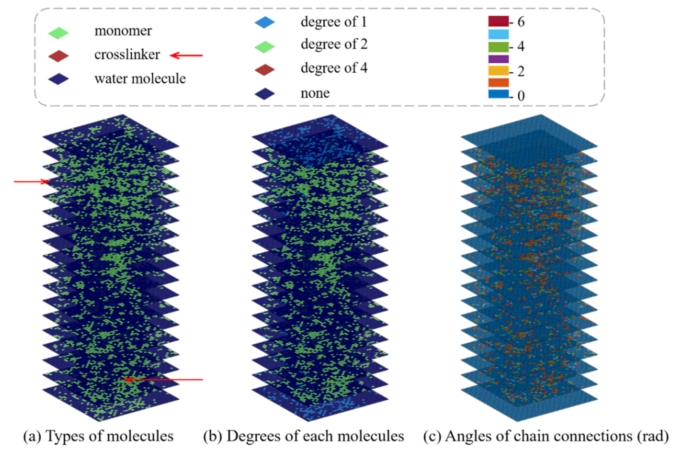
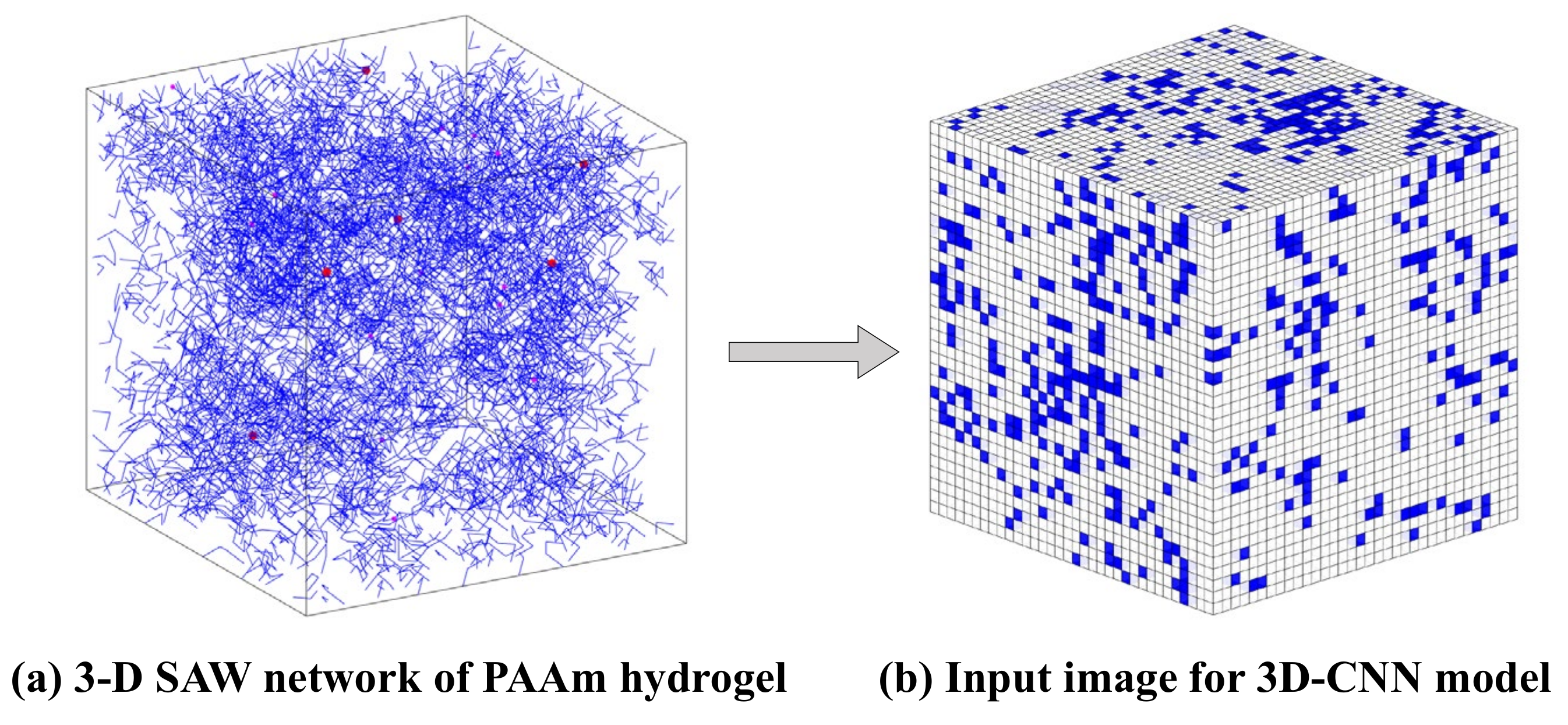
3.1. Dataset Generation and Preprocessing

The two deep learning models we developed are the DNN model and the 3D CNN model, respectively. It should be noted that the DNN in this study specifically refers to neural networks made up of fully connected layers (as the same architecture as MLP), to distinguish from CNN used in this study. For model comparison, we use theoretical resolution instead of experimental results as labels. Therefore, the outputs of the two models are not affected by experimental errors, which ensures the fair evaluations of the feasibility and performance of the DL models. Because each input data usually needs to maintain the same dimension for the DL models, the space size w is fixed at 33, and 2200 simulations are conducted using the SAW network model by changing the preset numbers of monomers and crosslinkers. As a result, the polymer mass fraction ϕ m is distributed from 5% to 80%, and the corresponding water content is from 95% to 20%. The number of samples and the space size have to be large enough to reflect the randomness and heterogeneity of the SAW network with different polymer mass fractions, but small enough to prevent excessive computational costs (considering that the input data of the 3D CNN model is four-dimensional, the amount of data will grow rapidly with the increase of the space size w ).
In the terms of the DNN model, the input data set is two-dimensional with one row per sample and one column per feature. We designed eight features in the DNN model to capture key physical information of the network generated by SAW. They are referred to as the number of chains, the number of monomers, the number of crosslinkers, the number of water molecules, the standard deviation of the number of monomers per chain, the number of isolated, branch, and network chains. As a result, the size of the input data of the DNN is 2176 × 8. There is a principle of feature design for the traditional MLP architecture, that is, each feature is possibly independent of other features, and potentially related to the outputs. Therefore, this is why we choose the standard deviation of the number of monomers per chain instead of the mean value (for the fifth feature), the latter can be calculated from the number of monomers (the second feature) and chains (the first feature). Similarly, the degree of cross-linking is also an important feature of the complex network structure of hydrogels, which can be calculated from the total number of monomers (the second feature) and the number of crosslinkers (the third feature). Therefore, they are no longer independent features. On the other hand, the original sample size of the 3D CNN model is 33 × 33 × 33. Through further transformation, the SAW network image is represented as a data structure that can train the 3D CNN model, as shown in Figure 8.
In order to include the geometric and physical information of the SAW network model in input data, we design three sublayers and combine them with the inputs by replacing the color channels in the traditional CNN architecture. The 3D CNN model we developed incorporates both the geometric and physical features of hydrogel networks for mechanical property prediction. More specifically, the geometric features captured by the sublayers are referred to as the types of molecules, the degree (the number of edges incident to the vertex) of each molecule, and the angles of chain connections, as shown in Figure 9.
As for the color channels of the input images in a typical CNN, they are generally composed of one (grayscale image) or three (colorful image with red, green, and blue, i.e., RGB) sublayers. However, the colors of input images in this study are only for representation and explanation. They have no specific physical meaning. As for the traditional CNN, the original values of a pixel range from 0 to 255, which would be exceedingly large for a CNN-based model. Therefore, the RGB values are rescaled into the range (0, 1) to speed up the convergence of a training process. This problem also occurs in the dataset with sublayers used in this study, thus the datasets to be used are normalized into the range of (0, 1) before training.
The proposed sublayers make full use of various data formats of SAW simulation outputs. Compared with the DNN model, the local spatial information of SAW network model is included in 3D CNN model. Two datasets are eventually constructed, one is two-dimensional including 2176 samples and 8 features for the DNN model, the other includes 2176 four-dimensional samples with a size of 33 × 33 × 33 × 3 including the three feature channels. The corresponding nominal stress–stretch data are generated through Equation (13). The general idea of sublayers design described here can be extended to any other desired component to obtain effective mechanical properties.

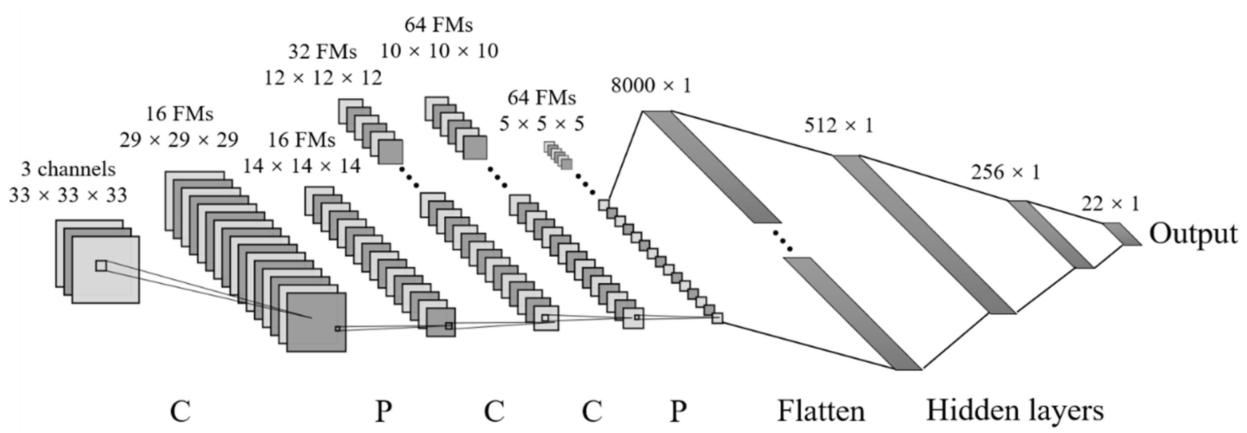
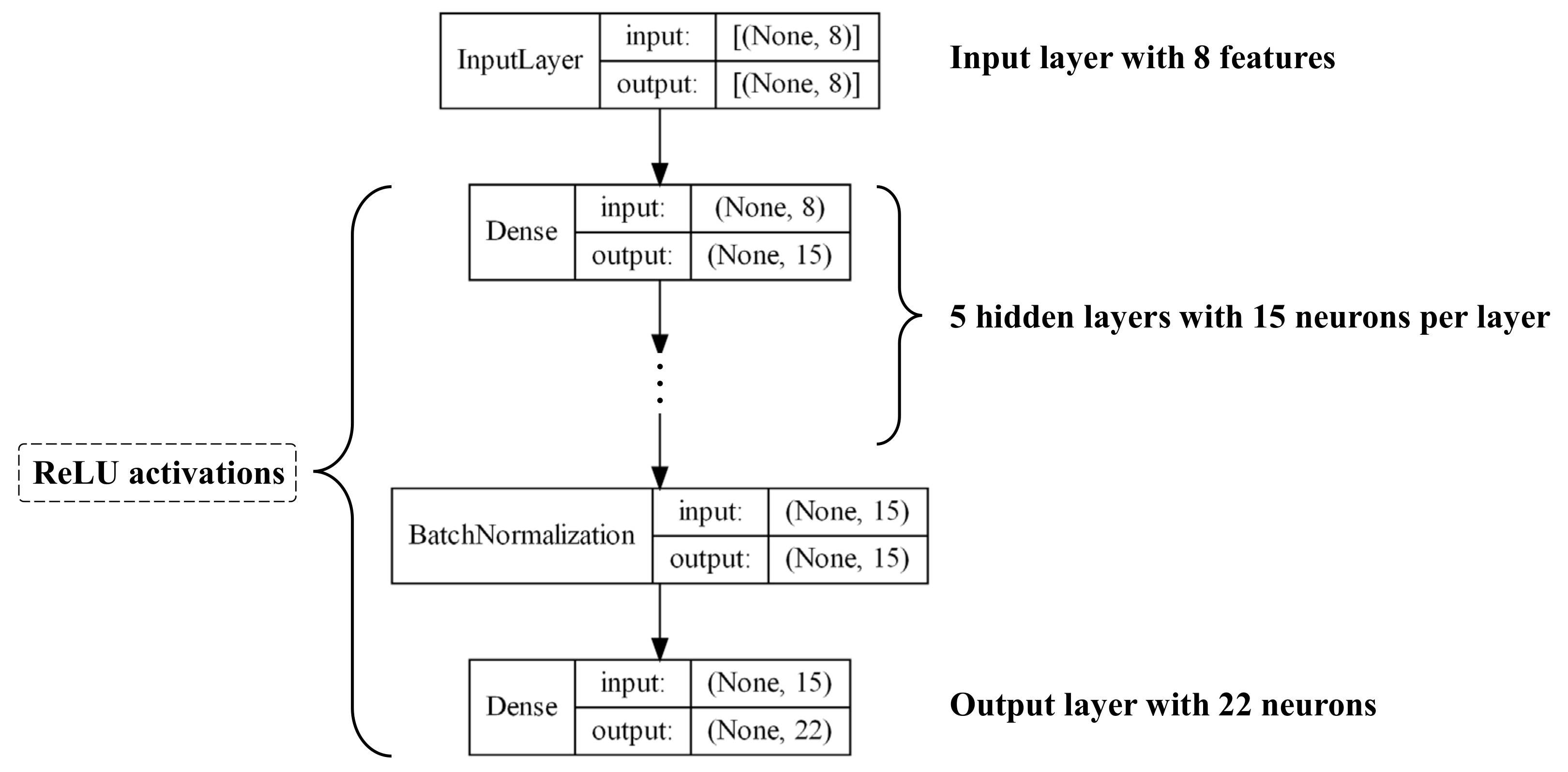
3.2. Framework of Deep Learning Models

On the basic paradigm of DL algorithms presented in previous section, we propose two architectures of the DL models, one is the DNN model based on MLP, the other is the 3D CNN model. Figure 10 gives the schematic illustration for the DNN architecture we have constructed. While Figure 11 provides a schematic of the 3D CNN architecture, where inputs are 3D images and outputs are the stress–stretch relations of single-network hydrogels under uniaxial tension.
The modeling starts from dividing both datasets into three parts, 70% for training, 10% for validation and 20% for testing. The hyperparameters used for the 3D CNN model are shown in Figure 11 and Table 1. Both models output a subsample of the stress–stretch curve, taking the stress values corresponding to 22 fixed stretching values. The dimensions of the output data are both equal to 22. It should be noted that when the stretch is small, the stretching points we selected are denser, and vice versa. Because on the one hand, nonlinear effect is more obvious at small stretch, and on the other hand, the neo-Hookean-based constitutive model has a larger error at large stretch.
The development of the two DL-based models is carried out on Python 3.8 and Keras with the Tensorflow backend. The training of 3D CNN is first to determine the number of convolutional, max-pooling, fully connected layers, and the hidden neurons in each layer (see Figure 11). The prediction of mechanical property is a regression task, so mean square error (MSE) is set as the loss function, which is referred as:
M S E = 1 m i = 1 m y ^ i y i 2
where m denotes the number of samples. y ^ i and y i are predicted and actual value of output, respectively. The optimizer of 3D CNN model takes ‘Nadam’ algorithm with a 0.001 learning rate. Following the input layer is a combination of the first convolution layer and max-pooling layer. There are sixteen convolution filters with a size of five in the first convolutional layer. Then two deeper convolutional with filters size of three and one max-pooling layer are followed sequentially. Considering the output is always positive (nominal stress), ReLU activation function is the best choice to reflect the nonlinear response of uniaxial tension test of hydrogel. Subsequently, a fully connected layer leads to the output of the network, which is the stress–stretch relationship. Once trained, the model is able to predict the relationship with an obviously shorter time (within one second) when fed by unseen input image. As for the DNN model, after a process of combining grid search [53] and cross validation in the hyperparameters space, the preferred hyperparameters of the model for mechanical property prediction problems are determined and detailed in Table 1. The stochastic gradient descent method is taken as the optimizer of the DNN model with a learning rate of 0.0056.

4. Results and Discussions

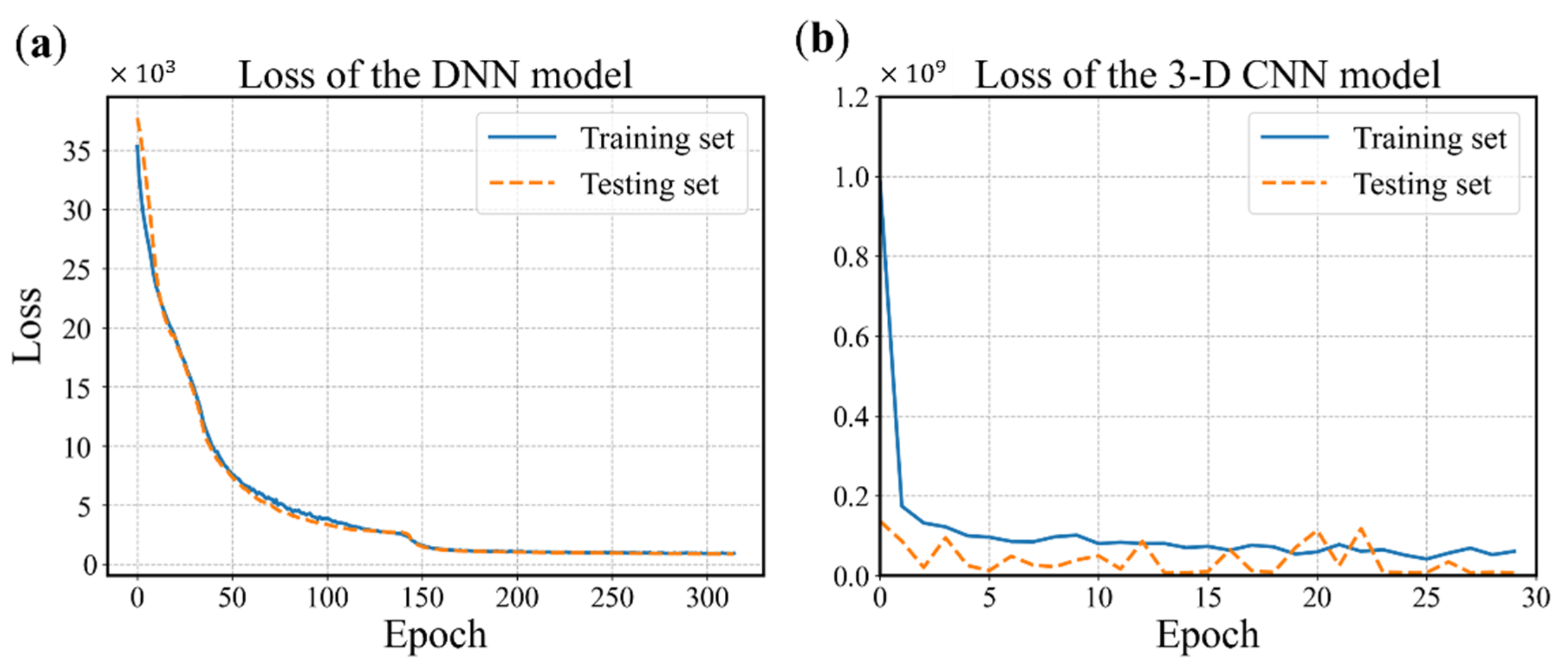
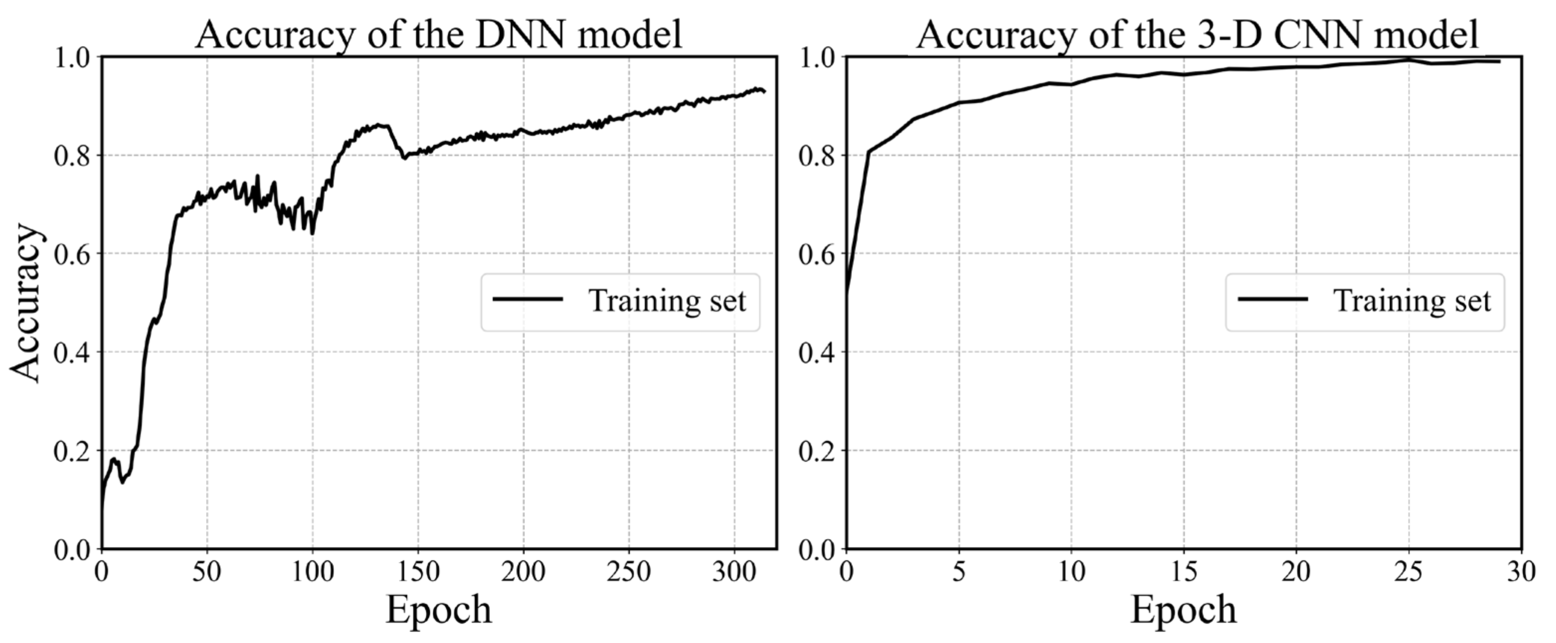
4.1. Analysis and Comparison of Model Performance

The configuration of the DNN model is determined using the grid search and cross validation, and the details are not mentioned here for simplicity. The configuration is shown in Figure 10 and the hyperparameters are listed in Table 1. It is worth mentioning that batch normalization is a technique for training deep neural networks that standardizes the inputs to a layer for each mini-batch [54]. Owning the effect of stabilizing the learning process and significantly reducing the number of training epochs required, batch normalization can normalize the prior inputs and ensure the gradients are more predictive, thus allow for larger range of learning rates and faster convergence. Figure 12 depicts the convergence history of training and testing set for each model. It can be seen from Figure 12a that the MSE losses of training set and testing set converge rapidly within 160 epochs, then maintain stable in the remaining epochs. One epoch can be explained as a batch of samples that goes forward from the input layer at the beginning then feeds back from the output layer to complete an iteration. When all training samples have completed one iteration, the epoch ends. The 3D CNN model is trained using 30 epochs with batch-size of 32 as shown in Figure 12b. The fluctuation of the loss may be caused by the following reasons. The first reason is that the learning rate is unchangeable in this model during the training process, whose value can be large enough to converge at the beginning, but too large to reach a stable and local minimum. As a result, the loss fluctuates around the ‘valley’ of the loss function. Secondly, there may be a reason that the loss function is exceedingly complex due to the high dimension and large amount of input data, and the optimizer is hard to find a good convergence point. The history of training accuracy is shown in Figure 13. Both the models we developed reach an accuracy over 90%.
By comparing the two figures in Figure 13, it is found that the accuracy of the 3D CNN model is more stable than the DNN model and is able to reach a higher value within fewer epochs. Because the number of trainable weights in the 3D CNN model is much more than the latter. The convolutional layers of our 3D CNN model focus on extracting the features of each image, while the hierarchical architecture could efficiently capture the potential feature maps relating to the outputs. Therefore, the 3D CNN model is able to reach a better convergence point on a more complex loss function.
It is noted that we employ a dropout layer after each hidden layer in the fully connected layer of the 3D CNN model. The effect of dropout on model’s performance is actually negative as usual, because lots of specific data are directly dropped. However, it can effectively reduce the possibility of model overfitting. By sacrificing some accuracy on the training set to obtain better accuracy on the testing set, the model is able to conduct better robustness and generalization on new data that was unseen before.
In order to quantitatively analyze the performance of the DNN and 3D CNN model, mean square error (MSE) and mean square percentage error (MSPE) are computed. MSPE for a selected set of data represents the percentage error between the predicted values and the ground truth calculated from the constitutive model. The MSPE used in this study is defined as:
M S P E = 1 m i = 1 m y ^ i y i y ¯ 2 × 100 %
where y ¯ denotes the average nominal stress of all the samples in the dataset. The MSE, MSPE and prediction accuracy R 2 of the two models we proposed are summarized in Table 2. It can be seen that the MSPE values of both models are no more than 4% and the R 2 values reach highly over 91%, which confirms that the 3D CNN model has more potential for the structure–property linkage problem. Besides, with only 1600 training samples, the proposed models can achieve quite gratifying performance. The 3D CNN model shows a remarkable ability to extract structural features of the network. The 3D CNN provides a direct and reliable method to identify the three-dimensional network information of single-network hydrogels at the mesoscopic scale, and has the capability to establish a highly accurate structure–property linkage. Our model can be used to predict the mechanical property based on the basic material structure, which is a universal method bridging the mesoscopic network to macroscopic mechanical properties.

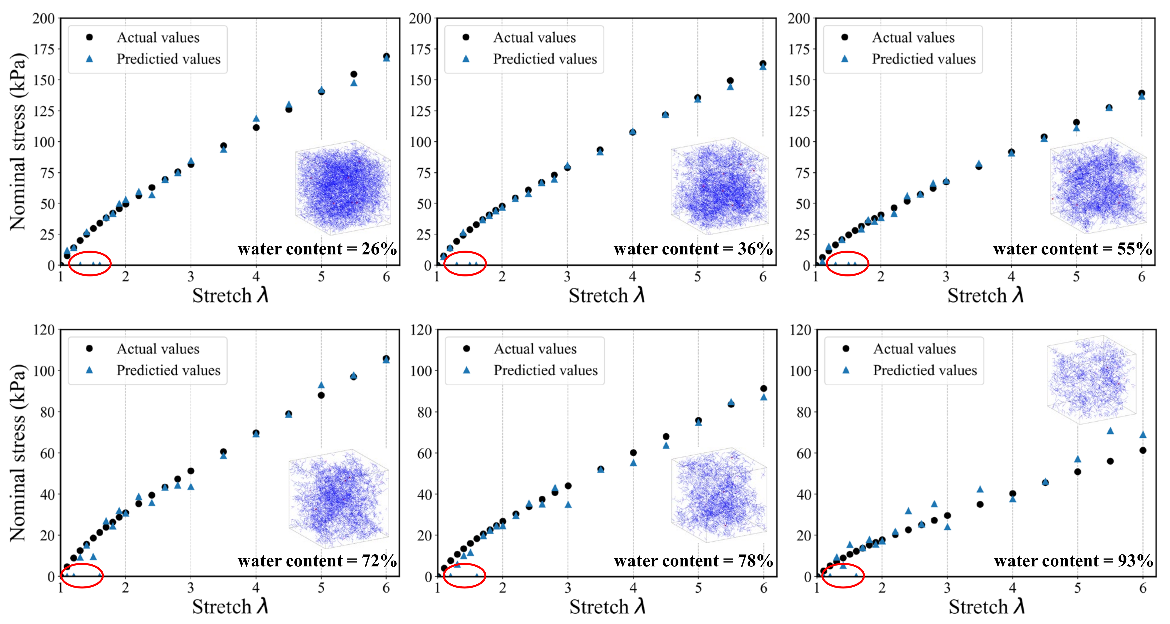
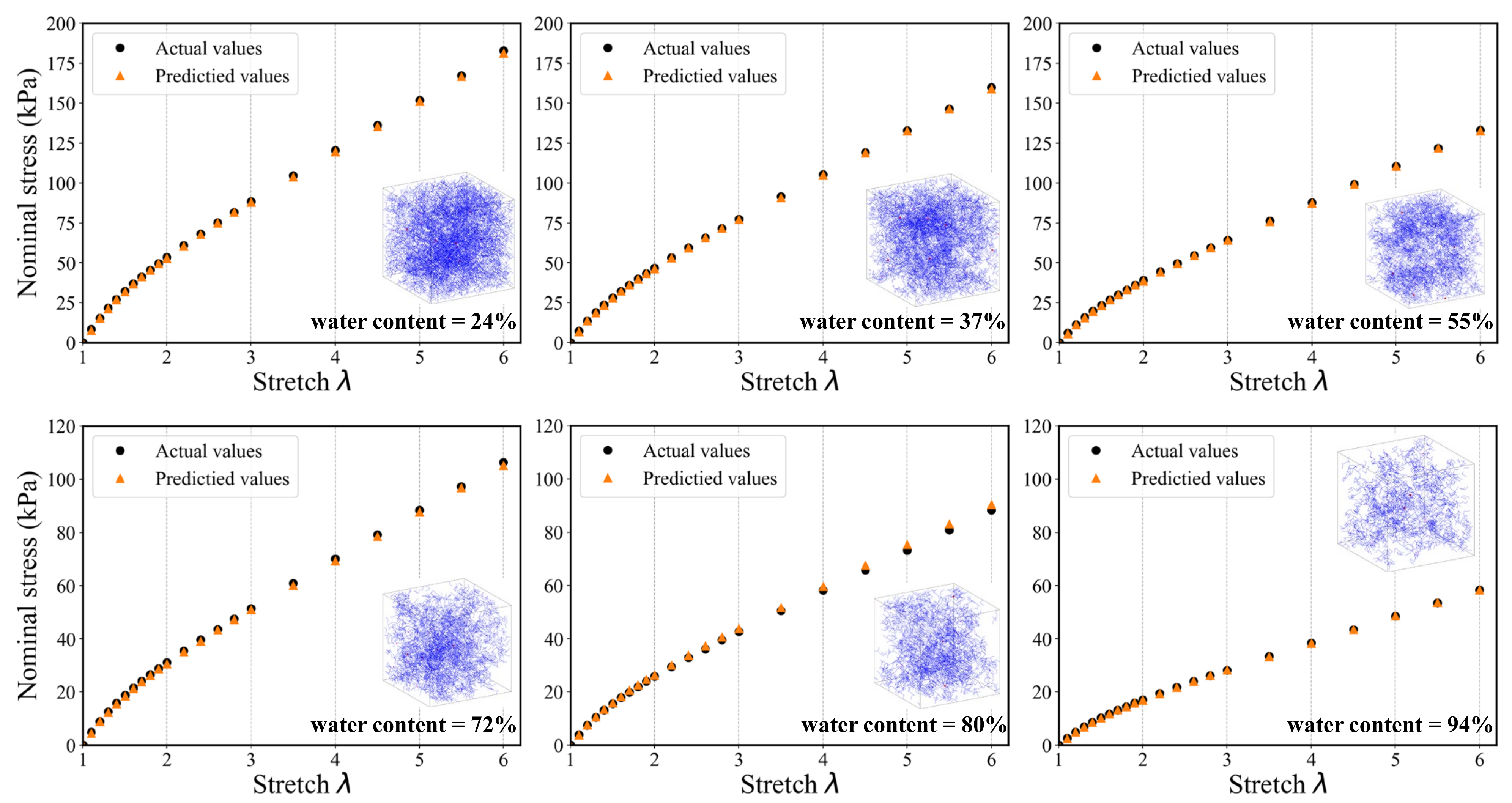
4.2. Evaluation of Model Generalization

Considering that the nominal stress–stretch curve is usually a comprehensive demonstration of mechanical properties, more specific descriptors such as modulus and strength can be derived from the relationship. Therefore, we decide to evaluate the model based on the mechanical response under uniaxial tension, and explore the potential of the proposed model in the issue of predicting mechanical properties.
Our model architecture is inspired by the recent full convolutional architecture in traditional computer vision applications. According to empirical observations, convolutional architecture is an efficient and stable method because it is a local operation, allowing itself to implicitly quantify and learn the local spatial effects of the mesoscopic network. Obtaining the performance of the DL-based model on unseen data is essential to ensure its compatibility of application. In order to test the generalization ability of the models, we utilize the SAW network model to newly generate multiple network models, and transform these new samples to input images for 3D CNN model according to the process described previously. Then we pass them to the models we proposed to predict the stress–stretch relationship.
To evaluate the generalization ability and robustness of the proposed DL-based modeling framework, Figure 14 and Figure 15 provide the comparisons between the predicted results and the actual results, respectively. It can be seen that both the two models keep good consistency. Despite the nonlinear behavior of the stress–stretch curve for hydrogel, they can fit a favorable nonlinear trend. There are 22 principle stretch values we firstly determined, and the predicted output could contain 22 corresponding nominal stress values. The model can accurately capture the initial nonlinear growth of the nominal stress. In the case of the DNN model, one can easily see that the predictions tend to be more accurate when the water content is low, which indicates that the DNN model has a better performance on the homogenous hydrogel network. With the increase of water content, the predictions become unstable and begin to distort. In addition, the distortion happens only in the first few data points. Because the weights of hidden layers more possibly tend to be close to zeros when labels are close to zeros. The traditional DNN extracts the features of the overall structure instead of the local structure, so its performance is not good enough in the prediction of heterogeneous polymer network. In the case of the 3D CNN model, the fitting accuracy of samples under different water content is significantly higher than that of DNN model. It is indicated that the admirable learning ability ensures 3D CNN to learn complex behavior patterns from the mesoscopic structure. It also has a high fidelity for sparsely heterogeneous and random networks. The prediction results of the two models show that the DL-based model can still accurately predict the mechanical property of the unseen samples of hydrogel network. The proposed modeling framework has good application prospects for multi-scale modeling.
To the best of our knowledge, this is the first time that a three-dimensional CNN is implemented to establish structure–property linkage of a single-network hydrogel based on the SAW model. Therefore, the proposed modeling framework in this study provides important insight and guidance, and the proposed model can serve as a pre-trained model to accelerate extensive prediction of mechanical properties, especially for the 3D complex structure. Besides, the DL-based modeling method described previously in this paper expands data-driven strategy to the soft material design and research of material property. It allows a more efficient determination of parameters in the mechanical model, such as the constitutive models, under the lack of experimental data sets. In addition, the ideas of sublayers design we present previously also guide how CNNs could be employed for problems in mechanics and other engineering disciplines. More mechanical properties (components of stiffness) in higher dimensions are required in the field of describing the mechanical behavior of materials. Given the success of 3D CNN model in our current 3D problem, it would be a promising strategy to identify various mechanical properties as different channels in a CNN input sublayer.

5. Conclusions

In order to predict the mechanical property of hydrogel, this paper firstly introduces the RW model, then develops a modeling method for the mesoscopic network of single-network hydrogels based on the SAW model with PAAm hydrogel as an example. Secondly, a DL-based modeling strategy is proposed on the basis of this approach. We developed two deep learning models, a DNN and a 3D CNN, respectively, for the construction of structure–property linkage of hydrogel. A grid search and cross validation of the hyperparameter space of the neural network architecture was employed to find the desirable DNN model, and eight features were designed to overall characterize the mesoscopic network model. In the 3D CNN model, feature extraction of 3D structure was achieved by designing the size of kernels and feature maps of the convolutional layers. It should be noted that we redesigned the color channels of the input images of the 3D CNN model to incorporate the physical and geometric information. The proposed 3D CNN model is able to learn input images that contain sublayers of physical information. These two models can quantitatively predict the relationship between mesoscopic network and the macroscopic mechanical properties. We trained the models using stress–stretch curves generated based on hydrogel theory and Neo-Hookean constitutive model, and then tested the generalization ability and robustness on the testing set. For the new SAW network samples, both DNN and 3D CNN models give accurate predictions, especially the 3D CNN shows a promising capability.
Furthermore, from the results of model evaluation, it can be found that the proposed DNN model can provide a good prediction for lower water content hydrogel, but it shows a large fluctuation error when water content is high, which indicates the weakness of the DNN model for inhomogeneous and sparse network polymer. In contrast, the 3D CNN performs more superior than the conventional DNN approach, which reflects the potential of the model in 3D polymer structural analysis problems. The 3D CNN can capture potential structural features of hydrogel, especially for multiscale material problems. The proposed method can be easily extended to study similar problems, such as the structural design and the material property design to improve the mechanical performance of different soft materials.

Author Contributions

Conceptualization, J.-A.Z.; methodology, J.-A.Z. and Y.J.; model building, J.-A.Z.; analysis, J.-A.Z. and Y.J.; writing—original draft preparation, J.-A.Z.; writing—review and editing, J.-A.Z., Y.J., J.L. and Z.L.; visualization, J.-A.Z.; supervision, Z.L.; project administration, Z.L.; funding acquisition, Z.L. All authors have read and agreed to the published version of the manuscript.

Funding

This work was supported by the National Natural Science Foundation of China [Grant Numbers 11820101001, 12172273].

Institutional Review Board Statement

Not applicable.

Informed Consent Statement

Not applicable.

Conflicts of Interest

The authors declare no conflict of interest.

References

  1. Liu, Z.; Toh, W.; Ng, T.Y. Advances in Mechanics of Soft Materials: A Review of Large Deformation Behavior of Hydrogels. Int. J. Appl. Mech. 2015, 7, 1530001. [Google Scholar] [CrossRef]
  2. Huang, R.; Zheng, S.; Liu, Z.; Ng, T.Y. Recent Advances of the Constitutive Models of Smart Materials—Hydrogels and Shape Memory Polymers. Int. J. Appl. Mech. 2020, 12, 2050014. [Google Scholar] [CrossRef] [Green Version]
  3. Sun, J.Y.; Zhao, X.H.; Illeperuma, W.R.K.; Chaudhuri, O.; Oh, K.H.; Mooney, D.J.; Vlassak, J.J.; Suo, Z.G. Highly stretchable and tough hydrogels. Nature 2012, 489, 133–136. [Google Scholar] [CrossRef] [PubMed]
  4. Wei, Z.; Yang, J.H.; Liu, Z.Q.; Xu, F.; Zhou, J.X.; Zrinyi, M.; Osada, Y.; Chen, Y.M. Novel Biocompatible Polysaccharide-Based Self-Healing Hydrogel. Adv. Funct. Mater. 2015, 25, 1352–1359. [Google Scholar] [CrossRef]
  5. Taylor, D.L.; Panhuis, M.I.H. Self-Healing Hydrogels. Adv. Mater. 2016, 28, 9060–9093. [Google Scholar] [CrossRef] [PubMed]
  6. Gong, J.P. Why are double network hydrogels so tough? Soft Matter 2010, 6, 2583–2590. [Google Scholar] [CrossRef]
  7. Li, J.; Mooney, D.J. Designing hydrogels for controlled drug delivery. Nat. Rev. Mater. 2016, 1, 16071. [Google Scholar] [CrossRef]
  8. Liu, L.; Li, X.; Ren, X.; Wu, G.F. Flexible strain sensors with rapid self-healing by multiple hydrogen bonds. Polymer 2020, 202, 122657. [Google Scholar] [CrossRef]
  9. Tian, K.; Bae, J.; Bakarich, S.E.; Yang, C.; Gately, R.D.; Spinks, G.M.; Panhuis, M.I.H.; Suo, Z.; Vlassak, J.J. 3D Printing of Transparent and Conductive Heterogeneous Hydrogel-Elastomer Systems. Adv. Mater. 2017, 29, 1604827. [Google Scholar] [CrossRef] [Green Version]
  10. Yuk, H.; Varela, C.E.; Nabzdyk, C.S.; Mao, X.; Padera, R.F.; Roche, E.T.; Zhao, X. Dry double-sided tape for adhesion of wet tissues and devices. Nature 2019, 575, 169–174. [Google Scholar] [CrossRef]
  11. Lyu, Y.; Azevedo, H.S. Supramolecular Hydrogels for Protein Delivery in Tissue Engineering. Molecules 2021, 26, 873. [Google Scholar] [CrossRef] [PubMed]
  12. Censi, R.; Di Martino, P.; Vermonden, T.; Hennink, W.E. Hydrogels for protein delivery in tissue engineering. J. Control. Release 2012, 161, 680–692. [Google Scholar] [CrossRef] [PubMed]
  13. Xing, J.; Yang, B.; Dang, W.; Li, J.; Bai, B. Preparation of Photo/Electro-Sensitive Hydrogel and Its Adsorption/Desorption Behavior to Acid Fuchsine. Water Air Soil Pollut. 2020, 231, 231. [Google Scholar] [CrossRef]
  14. Shuai, S.; Zhou, S.; Liu, Y.; Huo, W.; Zhu, H.; Li, Y.; Rao, Z.; Zhao, C.; Hao, J. The preparation and property of photo- and thermo-responsive hydrogels with a blending system. J. Mater. Sci. 2020, 55, 786–795. [Google Scholar] [CrossRef]
  15. Chen, X.; Li, H.; Lam, K.Y. A multiphysics model of photo-sensitive hydrogels in response to light-thermo-pH-salt coupled stimuli for biomedical applications. Bioelectrochemistry 2020, 135, 107584. [Google Scholar] [CrossRef] [PubMed]
  16. Xiao, R.; Qian, J.; Qu, S. Modeling Gel Swelling in Binary Solvents: A Thermodynamic Approach to Explaining Cosolvency and Cononsolvency Effects. Int. J. Appl. Mech. 2019, 11, 1950050. [Google Scholar] [CrossRef]
  17. Ghareeb, A.; Elbanna, A. An adaptive quasicontinuum approach for modeling fracture in networked materials: Application to modeling of polymer networks. J. Mech. Phys. Solids 2020, 137, 103819. [Google Scholar] [CrossRef] [Green Version]
  18. Tauber, J.; Kok, A.R.; van der Gucht, J.; Dussi, S. The role of temperature in the rigidity-controlled fracture of elastic networks. Soft Matter 2020, 16, 9975–9985. [Google Scholar] [CrossRef]
  19. Yin, Y.; Bertin, N.; Wang, Y.; Bao, Z.; Cai, W. Topological origin of strain induced damage of multi-network elastomers by bond breaking. Extrem. Mech. Lett. 2020, 40, 100883. [Google Scholar] [CrossRef]
  20. Lei, J.; Li, Z.; Xu, S.; Liu, Z. Recent advances of hydrogel network models for studies on mechanical behaviors. Acta Mech. Sin. 2021, 37, 367–386. [Google Scholar] [CrossRef]
  21. Lei, J.; Li, Z.; Xu, S.; Liu, Z. A mesoscopic network mechanics method to reproduce the large deformation and fracture process of cross-linked elastomers. J. Mech. Phys. Solids 2021, 156, 104599. [Google Scholar] [CrossRef]
  22. Dong, J.; Qin, Q.-H.; Xiao, Y. Nelder-Mead Optimization of Elastic Metamaterials via Machine-Learning-Aided Surrogate Modeling. Int. J. Appl. Mech. 2020, 12, 2050011. [Google Scholar] [CrossRef]
  23. Jie, Y.; Rui, X.; Qun, H.; Qian, S.; Wei, H.; Heng, H. Data-driven Computational Mechanics:a Review. Chin. J. Solid Mech. 2020, 41, 1–14. [Google Scholar]
  24. Bessa, M.A.; Bostanabad, R.; Liu, Z.; Hu, A.; Apley, D.W.; Brinson, C.; Chen, W.; Liu, W.K. A framework for data-driven analysis of materials under uncertainty: Countering the curse of dimensionality. Comput. Methods Appl. Mech. Eng. 2017, 320, 633–667. [Google Scholar] [CrossRef]
  25. Ibanez, R.; Abisset-Chavanne, E.; Aguado, J.V.; Gonzalez, D.; Cueto, E.; Chinesta, F. A Manifold Learning Approach to Data-Driven Computational Elasticity and Inelasticity. Arch. Comput. Methods Eng. 2018, 25, 47–57. [Google Scholar] [CrossRef] [Green Version]
  26. Zheng, S.; Liu, Z. The Machine Learning Embedded Method of Parameters Determination in the Constitutive Models and Potential Applications for Hydrogels. Int. J. Appl. Mech. 2021, 13, 2150001. [Google Scholar] [CrossRef]
  27. Li, F.; Han, J.; Cao, T.; Lam, W.; Fan, B.; Tang, W.; Chen, S.; Fok, K.L.; Li, L. Design of self-assembly dipeptide hydrogels and machine learning via their chemical features. Proc. Natl. Acad. Sci. USA 2019, 116, 11259–11264. [Google Scholar] [CrossRef] [Green Version]
  28. Haghighat, E.; Raissi, M.; Moure, A.; Gomez, H.; Juanes, R. A physics-informed deep learning framework for inversion and surrogate modeling in solid mechanics. Comput. Methods Appl. Mech. Eng. 2021, 379, 113741. [Google Scholar] [CrossRef]
  29. Pavel, M.S.; Schulz, H.; Behnke, S. Object class segmentation of RGB-D video using recurrent convolutional neural networks. Neural Netw. 2017, 88, 105–113. [Google Scholar] [CrossRef]
  30. Yu, S.; Jia, S.; Xu, C. Convolutional neural networks for hyperspectral image classification. Neurocomputing 2017, 219, 88–98. [Google Scholar] [CrossRef]
  31. Shin, H.-C.; Roth, H.R.; Gao, M.; Lu, L.; Xu, Z.; Nogues, I.; Yao, J.; Mollura, D.; Summers, R.M. Deep Convolutional Neural Networks for Computer-Aided Detection: CNN Architectures, Dataset Characteristics and Transfer Learning. IEEE Trans. Med Imaging 2016, 35, 1285–1298. [Google Scholar] [CrossRef] [Green Version]
  32. Khan, A.; Sohail, A.; Zahoora, U.; Qureshi, A.S. A survey of the recent architectures of deep convolutional neural networks. Artif. Intell. Rev. 2020, 53, 5455–5516. [Google Scholar] [CrossRef] [Green Version]
  33. Zobeiry, N.; Reiner, J.; Vaziri, R. Theory-guided machine learning for damage characterization of composites. Compos. Struct. 2020, 246, 112407. [Google Scholar] [CrossRef]
  34. Abueidda, D.W.; Almasri, M.; Ammourah, R.; Ravaioli, U.; Jasiuk, I.M.; Sobh, N.A. Prediction and optimization of mechanical properties of composites using convolutional neural networks. Compos. Struct. 2019, 227, 111264. [Google Scholar] [CrossRef] [Green Version]
  35. Yang, C.; Kim, Y.; Ryu, S.; Gu, G.X. Prediction of composite microstructure stress-strain curves using convolutional neural networks. Mater. Des. 2020, 189, 108509. [Google Scholar] [CrossRef]
  36. Yang, Z.; Yabansu, Y.C.; Al-Bahrani, R.; Liao, W.-K.; Choudhary, A.N.; Kalidindi, S.R.; Agrawal, A. Deep learning approaches for mining structure-property linkages in high contrast composites from simulation datasets. Comput. Mater. Sci. 2018, 151, 278–287. [Google Scholar] [CrossRef]
  37. Cecen, A.; Dai, H.; Yabansu, Y.C.; Kalidindi, S.R.; Song, L. Material structure-property linkages using three-dimensional convolutional neural networks. Acta Mater. 2018, 146, 76–84. [Google Scholar] [CrossRef]
  38. Yang, Z.; Papanikolaou, S.; Reid, A.C.E.; Liao, W.K.; Choudhary, A.N.; Campbell, C.; Agrawal, A. Learning to Predict Crystal Plasticity at the Nanoscale: Deep Residual Networks and Size Effects in Uniaxial Compression Discrete Dislocation Simulations. Sci. Rep. 2020, 10, 8262. [Google Scholar] [CrossRef] [PubMed]
  39. Pandey, A.; Pokharel, R. Machine learning based surrogate modeling approach for mapping crystal deformation in three dimensions. Scr. Mater. 2021, 193, 1–5. [Google Scholar] [CrossRef]
  40. Herriott, C.; Spear, A.D. Predicting microstructure-dependent mechanical properties in additively manufactured metals with machine- and deep-learning methods. Comput. Mater. Sci. 2020, 175, 109599. [Google Scholar] [CrossRef]
  41. Choi, J.; Quagliato, L.; Lee, S.; Shin, J.; Kim, N. Multiaxial fatigue life prediction of polychloroprene rubber (CR) reinforced with tungsten nano-particles based on semi-empirical and machine learning models. Int. J. Fatigue 2021, 145, 106136. [Google Scholar] [CrossRef]
  42. Douglass, M.J.J. Hands-on Machine Learning with Scikit-Learn, Keras, and Tensorflow, 2nd edition. Phys. Eng. Sci. Med. 2020, 43, 1135–1136. [Google Scholar] [CrossRef]
  43. Flory, P.J.; Rehner, J. Statistical mechanics of cross-linked polymer networks I Rubberlike elasticity. J. Chem. Phys. 1943, 11, 512–520. [Google Scholar] [CrossRef]
  44. Flory, P.J.; Rehner, J. Statistical mechanics of cross-linked polymer networks II Swelling. J. Chem. Phys. 1943, 11, 521–526. [Google Scholar] [CrossRef]
  45. Li, Z.; Liu, Z.; Ng, T.Y.; Sharma, P. The effect of water content on the elastic modulus and fracture energy of hydrogel. Extrem. Mech. Lett. 2020, 35, 100617. [Google Scholar] [CrossRef]
  46. Li, Z.; Liu, Z. Energy transfer speed of polymer network and its scaling-law of elastic modulus—New insights. J. Appl. Phys. 2019, 126, 215101. [Google Scholar] [CrossRef] [Green Version]
  47. Liu, R.; Kumar, A.; Chen, Z.; Agrawal, A.; Sundararaghavan, V.; Choudhary, A. A predictive machine learning approach for microstructure optimization and materials design. Sci. Rep. 2015, 5, 11551. [Google Scholar] [CrossRef] [Green Version]
  48. Reimann, D.; Nidadavolu, K.; ul Hassan, H.; Vajragupta, N.; Glasmachers, T.; Junker, P.; Hartmaier, A. Modeling Macroscopic Material Behavior With Machine Learning Algorithms Trained by Micromechanical Simulations. Front. Mater. 2019, 6, 181. [Google Scholar] [CrossRef] [Green Version]
  49. Bag, S.; Mandal, R. Interaction from structure using machine learning: In and out of equilibrium. Soft Matter 2021, 17, 8322–8330. [Google Scholar] [CrossRef] [PubMed]
  50. Swaddiwudhipong, S.; Hua, J.; Harsono, E.; Liu, Z.S.; Ooi, N.S.B. Improved algorithm for material characterization by simulated indentation tests. Model. Simul. Mater. Sci. Eng. 2006, 14, 1347–1362. [Google Scholar] [CrossRef]
  51. Benitez, J.M.; Castro, J.L.; Requena, I. Are artificial neural networks black boxes? IEEE Trans. Neural Netw. 1997, 8, 1156–1164. [Google Scholar] [CrossRef] [PubMed]
  52. Hornik, K.; Stinchcombe, M.; White, H. Multilayer feedforward networks are universal approximators. Neural Netw. 1989, 2, 359–366. [Google Scholar] [CrossRef]
  53. Bergstra, J.; Bengio, Y. Random Search for Hyper-Parameter Optimization. J. Mach. Learn. Res. 2012, 13, 281–305. [Google Scholar]
  54. Santurkar, S.; Tsipras, D.; Ilyas, A.; Madry, A. How Does Batch Normalization Help Optimization? In Proceedings of the 32nd International Conference on Advances in Neural Information Processing Systems 31 (NIPS 2018), Montreal, QC, Canada, 3–8 December 2018. [Google Scholar]
Figure 1. Schematics of RW model and SAW model. (The red dot is the starting point, the black arrow represents the walking path, and the blue arrow represents the optional direction for the next step.) (a) The RW model. There are four optional directions at every moment. (b) The SAW model cannot go back. (c) The SAW model cannot select points that are already occupied.
Mathematics 09 02804 g001
Figure 2. The SAW path generated by the computer program. As the number of steps N increases, the configuration of the path is similar to the real polymer chain.
Mathematics 09 02804 g002
Figure 3. Schematics of SAW network generation model in 2D space. (a) The probability of what kind of particles to be inserted depends on the number of remaining monomers and crosslinkers. (b) Generation of new chain ends when inserting a crosslinker. (c) More chains walk in space to form a network.
Mathematics 09 02804 g003
Figure 4. Configurations of PAAm hydrogels generated by SAW network model.
Mathematics 09 02804 g004
Figure 5. Process of a single neuron in MLP.
Mathematics 09 02804 g005
Figure 6. Plot illustrating the sigmoid and ReLU activation functions.
Mathematics 09 02804 g006
Figure 7. Computation process of an example architecture of 2D CNN with 3 × 3 kernel (it should be noted that the process of bias and activation functions is ignored here for simple illustration). (a) Convolutional operation of the input image. The value in the receptive field is multiplied by the value of the corresponding center symmetric position in the kernel and then obtain the summed value in the feature maps. (b) 2 × 2 max-pooling process. Each 2 × 2 block is replaced by the maximum value in the receptive field. (c) Flatten last feature maps to one-dimension vector for learning.
Mathematics 09 02804 g007
Figure 8. Data representation for model training.
Mathematics 09 02804 g008
Figure 9. Schematics of slices plot illustration of three sublayers incorporating the geometric and physical features. (a) Representation of the type of molecules. (b) The degree of each molecule, that is, the number of connections per molecule. (c) The angle of chain connections.
Mathematics 09 02804 g009
Figure 10. Architecture schematic of the DNN model.
Mathematics 09 02804 g010
Figure 11. Three-dimensional convolutional neural network architecture (for simpler schematics, one gray rectangular represents one 3D input image). C is referred to as convolutional layer, P is max-pooling layer, and FMs denote the feature maps.
Mathematics 09 02804 g011
Figure 12. History of loss values. (a) The DNN model with 315 epochs. (b) The 3D CNN model with 30 epochs (0 to 29).
Mathematics 09 02804 g012
Figure 13. History of accuracy values.
Mathematics 09 02804 g013
Figure 14. A randomly generated set of six SAW models and corresponding stress–stretch curves for the DNN model prediction compared to the actual results. (The data points in the red circle represent prediction distortion).
Mathematics 09 02804 g014
Figure 15. A randomly generated set of six SAW models and corresponding stress–stretch curves for the 3D CNN model prediction compared to the actual results.
Mathematics 09 02804 g015
Table 1. Hyperparameters values used in the proposed models.
HyperparametersModel
DNN3D CNN
Number of epochs31530
Batch size3232
Learning rate5.6 × 10−31 × 10−3
OptimizerSGDNadam
Loss functionMSEMSE
Trainable weights1477430,872,6
Activation functionsReLUReLU
Table 2. Evaluation indicators of the deep learning models.
ModelValues of Indicators
Training SetTesting Set
MSEMSPE R 2 MSEMSPE R 2
DNN9.3 × 103 kPa3.61%92.87%9.1 × 10⁴ kPa3.55%91.00%
3D CNN7.1 × 103 kPa0.30%99.23%5.7 × 10³ kPa0.24%99.65%
Publisher’s Note: MDPI stays neutral with regard to jurisdictional claims in published maps and institutional affiliations.

