Extended Generalized Sinh-Normal Distribution

Abstract

Positively skewed data sets are common in different areas, and data sets such as material fatigue, reaction time, neuronal reaction time, agricultural engineering, and spatial data, among others, need to be fitted according to their features and maintain a good quality of fit. Skewness and bimodality are two of the features that data sets like this could present simultaneously. So, flexible statistical models should be proposed in this sense. In this paper, a general extended class of the sinh-normal distribution is presented. Additionally, the asymmetric distribution family is extended, and as a natural extension of this model, the extended Birnbaum–Saunders distribution is studied as well. The proposed model presents a better goodness of fit compared to the other studied models.

1. Introduction

When materials are exposed to pressure or stress levels, material structural damage could occur. This is known as material fatigue, and a statistical model to fit random variables to model the failure time of fatigue for material was proposed by Birnbaum and Saunders (1969) [1], known in the literature as Birnbaum–Saunders distribution and generally denoted by $BS(\alpha ,\beta )$, where $\alpha >0$ represents a shape parameter and $\beta >0$ is a scale parameter and the median of the distribution. Later, Desmond (1985) [2] showed that the BS distribution describes the time failure that occurs when some kind of damage is accumulated after a given time.

A distribution associated with that of Birnbaum and Saunders (BS) is the sinh-normal (SHN) distribution. This distribution, introduced by Rieck and Nederman (1991) [3], is based on a nonlinear transformation of a normal distribution. Therefore, let $Z=\frac{2}{\alpha }sinh\left(\frac{Y-\xi }{\sigma }\right)\sim N(0,1),$ where $\xi$ and $\sigma$ are location and scale parameters, respectively, and $\alpha$ is a shape parameter. Then, random variable (r.v.) Y follows a sinh-normal distribution denoted by $SHN(\alpha ,\xi ,\sigma )$. A probability density function (pdf) of a random variable with a SHN distribution is given by

$$f\left(z\right)=b_y^{\prime }\varphi \left(b_y\right),$$

(1)

where $b_y=b(y,\alpha ,\xi ,\sigma )=\frac{2}{\alpha }\sinh \left(\frac{y-\xi }{\sigma }\right)$, $b_y^{\prime }=\frac{2}{\alpha \sigma }\cosh \left(\frac{y-\xi }{\sigma }\right)$ is a derivative of $b_y$ with respect to y, and $\varphi (.)$ is the pdf of the normal distribution. It can be shown that the s-th moment of a random variable with a SHN distribution is given by

$${\mu }_s=\mathbb{E}\left(Y^s\right)=\sum _{k=0}^s\left(\genfrac{}{}{0pt}{}{s}{k}\right){\sigma }^k{\xi }^{s-k}{c}_k\left(\alpha \right),$$

(2)

where

$$c_k\left(\alpha \right)={\int }_{-\infty }^{\infty }{\left({sinh}^{-1}\left(\frac{\alpha }{2}w\right)\right)}^k\varphi \left(w\right)dw.$$

(3)

From this result, we obtain that ${\mu }_1=\mathbb{E}\left(Y\right)=\xi ,$ ${\mu }_2={\xi }^2+{\sigma }^2{c}_2\left(\alpha \right)$ and $var\left(Y\right)={\sigma }^2{c}_2\left(\alpha \right)$. It can also be shown, from the two central moments, that $\mathbb{E}{(Y-\xi )}^3=0$ is a symmetric distribution with respect to $\xi$. In general, we find that

$$\mathbb{E}{(Y-\xi )}^s={\sigma }^s{c}_s\left(\alpha \right).$$

(4)

Asymmetric extensions of the SHN model have been considered, for instance, by Leiva et al. (2010) ([4]) and Lemonte et al. (2011) ([5]), who studied the skewed SHN model, as well as by Martínez-Flórez et al. (2017) [6], who investigated the power SHN model, and Moreno-Arenas et al. (2016) [7], who presented the Proportional Hazard BS model (PHBS).

The SHN distribution is also known as the log-Birnbaum–Saunders (LBS) distribution because $Y\sim \mathrm{SHN}(\alpha ,\xi ,\sigma =2)$, then $T=exp\left(Y\right)$ follows a BS distribution, with parameters $\alpha$ and $\beta =exp\left(\xi \right).$

The pdf of a random variable $T\sim BS(\alpha ,\beta )$ is given by

$$\begin{array}{c}\hfill f\left(t\right)=\varphi \left(a_t\right)a_t^{\prime }t>0,\end{array}$$

(5)

where

$$\begin{array}{c}\hfill a_t=a_t(\alpha ,\beta )=\frac{1}{\alpha }\left(\sqrt{\frac{t}{\beta }}-\sqrt{\frac{\beta }{t}}\right),and{a}_t^{\prime }=a_t^{\prime }(\alpha ,\beta )=\frac{d{a}_t}{dt}=\frac{t^{-3/2}(t+\beta )}{2\alpha {\beta }^{1/2}}.\end{array}$$

(6)

An important feature of this distribution is its robustness concerning the estimation of its parameters—an aspect that was analyzed by Barros, Paula, and Leiva (2010) [8]. Moreover, extensions of this distribution to an elliptical family and to a skew elliptical family (this latter is known as the double generalized BS distribution) have been studied by Díaz-García et al. (2005) [9] and by Vilca-Labra and Leiva-Sánchez (2006) [10], respectively. Martínez-Flórez et al. [11] present an extension to a power-skew-elliptical family. Other types of extensions have also been considered by authors such as Castillo et al. (2011) [12], Cordeiro and Lemonte. (2014) [13], and Reyes et al. (2018) [14].

All these extensions are particularly characterized by fitting skew unimodal data while not being appropriate to fit bimodal data. However, Martinez-Florez et al. (2017) [6] and Olmos et al. (2017) [15] recently presented BS models to fit positive bimodal data. Likewise, Bolfarine et al. (2011) [16] introduced another model to fit positive bimodal data generated by the log-skew-normal distribution.

Cortés et al. (2018) [17] presented a class of extended distribution, generated by the pdf, $g\left(x\right)$, of the bimodal-normal distribution. They specifically defined a general class of distributions with a pdf given by

$$f\left(x\right)=\left(\frac{1+ϵh\left(x\right)}{1+ϵ\kappa }\right)g\left(x\right),$$

(7)

where $g\left(x\right)$ is a pdf, $ϵ\ge 0$ is a shape parameter, and h is a continuous positive function such that $\kappa ={\mathbb{E}}_g\left(h\left(X\right)\right)<\infty .$ This distribution is called the “general class of distributions”. Further, the authors study the normal, t-student, Laplace, and BS distributions as special cases. As special cases of this family, from Elal-Olivero et al. (2010) [18] and the bimodal log-skew-normal of Bolfarine et al. (2011) [16], the class of bimodal skew-elliptical distributions can be found in the literature.

In this study, we analyze and study a general extended class of the SHN distributions, which has an extra parameter to the SHN model and introduces flexibility to the SHN distribution. Additionally, an extension of the BS model is presented. We highlight that this kind of model could be applied to data sets related to material fatigue [2], reaction and neuronal reaction time [19], agricultural engineering [20], and spatial data (see [21,22], among others). Note that this distribution can fit bimodal data sets, which could be present in problems where the population is divided by groups such as gender or different levels of HIV-RNA.

This paper unfolds as follows: Section 2 presents the extended sinh-normal distribution (ESHN) model. Section 3 provides the statistical approximation of the moments of an ESHN random variable. Section 4 outlines the properties of the extended generalized sinh-normal (EGSHN) distribution. Section 5 shows the features of the extended sinh-normal regression model. Section 6 presents the results of a simulation study to analyze the properties of the EGSHN model. Section 7 develops two numerical illustrations to evaluate the relevance of the EGSHN. Section 8 discusses the statistical and practical implications of the proposed distribution.

2. Extended Sinh-Normal Distribution

We now propose an extension of the SHN case introduced by Rieck and Nederman (1991) [3] to a general class of distributions. Then, taking $h\left(y\right)=b_y^2$ and $g\left(y\right)=b_y^{\prime }\varphi \left(b_y\right)$ in equation (7), where $b_y$ and $b_y^{\prime }$ are defined as in (1), the extended class of SHN distribution is defined through the pdf given by

$$f\left(y\right)=\frac{1+\gamma b_y^2}{1+\gamma }{b}_y^{\prime }\varphi \left(b_y)\right),$$

(8)

with $\xi \in \mathbb{R}$ and $\alpha ,\sigma >0$ defined as the SHN distribution of Rieck and Nederman (1991) [3], and $\gamma \in \mathbb{R}+$ as a shape parameter. This distribution is denoted by $ESHN(\alpha ,\xi ,\sigma ,\gamma )$, which, for some values of the $\gamma$ parameter, could be bimodal. In this context, $\gamma$ could be considered as a bimodality parameter. It can be easily deduced that for $\gamma =0$, the SHN distribution is obtained, and if $\gamma \to \infty$, then $f\left(y\right)\to b_y^2{b}_y^{\prime }\varphi \left(b_y\right),$ which is a new family of distributions. It can be also shown that a random variable

$$b_Y=\frac{2}{\alpha }sinh\left(\frac{Y-\xi }{\sigma }\right)\sim EN,$$

where $EN$ is the extended normal distribution, as studied by Cortés et al. (2018) [17].

Denoting $Z=\frac{2}{\alpha }\frac{Y-\xi }{\sigma },$ then, we find that $\frac{Y-\xi }{\sigma }=\frac{\alpha }{2}Z$; thus, when $\alpha \to 0$, then $b_y\to z,$ $b_y^{\prime }\to 1$ and $b_y^{\prime }\varphi \left(b_y\right)\stackrel{D}{\sim }\varphi \left(z\right),$ where $\varphi \left(z\right)\equiv N(0,1)$ (see Rieck et al. [3]). Next, it is possible to conclude that when $\alpha \to 0,$ then $f\left(y\right)\sim EN.$

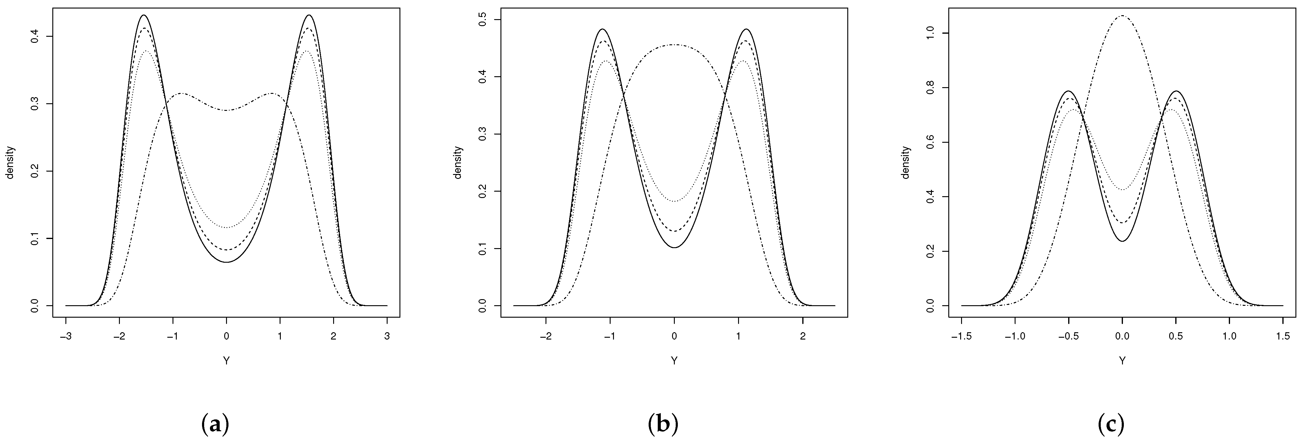
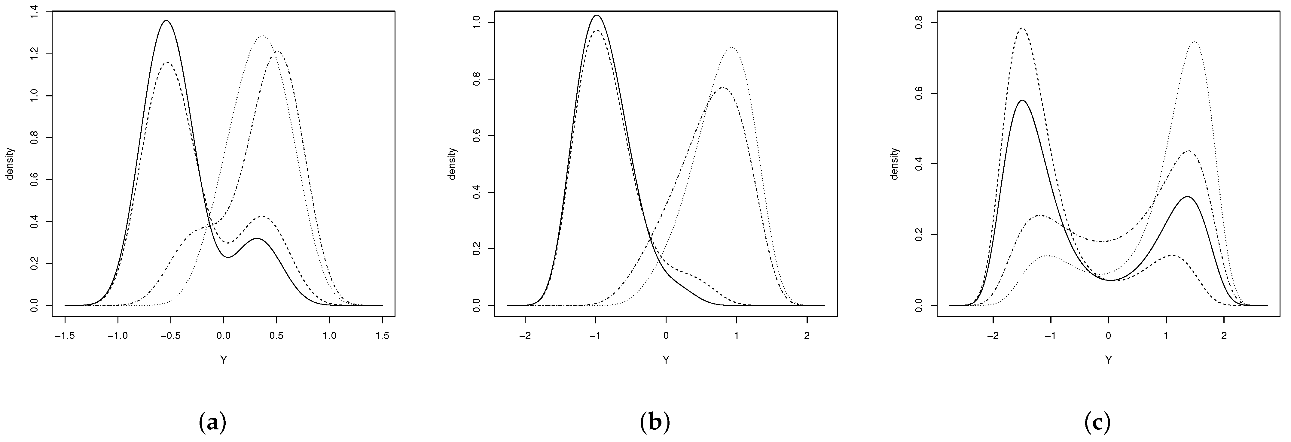
Figure 1 shows the pdf for an extended sinh-normal (ESHN) distribution with two parameters, respectively, where it can be seen that the distribution, for $\gamma =0$, is symmetric and unimodal in cases (b) and (c), and for the other cases, it is strongly bimodal.

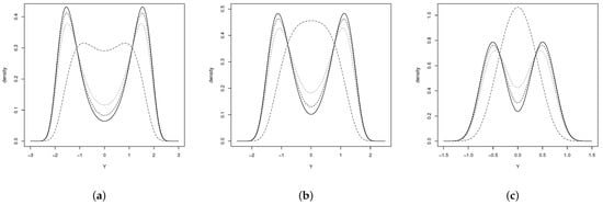
Figure 1. Distribution (a) $ESHN(2.75,0,1,\gamma )$ for $\gamma =3.5$ (solid line), $\gamma =2.5$ (dashed line), $\gamma =1.5$ (dotted line) y $\gamma =0$ (dash-dotted line), (b) $ESHN(1.75,0,1,\gamma )$ for $\gamma =3.5$ (solid line), $\gamma =2.5$ (dashed line), $\gamma =1.5$ (dotted line) and $\gamma =0$ (dash-dotted line) and (c) $ESHN(0.75,0,1,\gamma )$ for $\gamma =3.5$ (solid line), $\gamma =2.5$ (dashed line), $\gamma =1.5$ (dotted line) and $\gamma =0$ (dash-dotted line).

Denoting $p=\frac{1}{1+\gamma }$ and $1-p=\frac{\gamma }{1+\gamma },$ then, the pdf of $ESHN(\alpha ,\xi ,\sigma ,\gamma )$ could be written as a mixture of two distributions:

$$f\left(y\right)=p{b}_y^{\prime }\varphi \left(b_y\right)+(1-p)b_y^2{b}_y^{\prime }\varphi \left(b_y\right).$$

(9)

From (9) and remembering that a cumulative distribution function (cdf) of $SHN(\alpha ,\xi ,\sigma )$ is given by $\mathsf{\Phi }\left(b_y\right)$, then it can be shown that the cdf of the $ESHN(\alpha ,\xi ,\sigma ,\gamma )$ distribution is given by

$$\begin{array}{c}\hfill F\left(y\right)=\frac{1}{1+\gamma }\mathsf{\Phi }\left(b_y\right)+\frac{\gamma }{1+\gamma }{\int }_{-\infty }^{b_y}{z}^2\varphi \left(z\right)dz=\mathsf{\Phi }\left(b_y\right)-\frac{\gamma }{1+\gamma }{b}_y\varphi \left(b_y\right).\end{array}$$

(10)

Thus, the survival, risk (or hazard), and inverse risk functions of this distribution are, respectively, given by

$$S\left(t\right)=S_{SHN}\left(t\right)+\frac{\gamma }{1+\gamma }{b}_t\varphi \left(b_t\right),$$

and

$$h\left(t\right)=\frac{(1+\gamma b_t^2)h_{SHN}\left(t\right)}{(1+\gamma )+\sigma \gamma tanh\left(z\right)h_{SHN}\left(t\right)}\mathrm{and}R\left(t\right)=\frac{(1+\gamma b_t^2)R_{SHN}\left(t\right)}{(1+\gamma )-\sigma \gamma tanh\left(z\right)R_{SHN}\left(t\right)},$$

where $z=\frac{t-\xi }{\sigma },$ $b_t$ is defined as $b_y$, with $S_{SHN},$ $h_{SHN}\left(t\right)$, and $R_{SHN}\left(t\right)$ being the survival, hazard and inverse risk functions of the model $SHN(\alpha ,\xi ,\sigma ).$

Another important result of this distribution is presented as follows:

Let $Y\sim ESHN(\alpha ,\xi ,2,\gamma )$; then, the random variable $T=exp\left(Y\right)$ follows an $EBS(\alpha ,\beta ,\gamma )$ distribution, and where $\beta =exp\left(\xi \right)$ and $EBS$ is related to the extended BS distribution, whose properties and moments are studied in Cortés et al. (2018) [17]. So, if $T\sim EBS(\alpha ,\beta ,\gamma )$, then (i) $aT\sim EBS(\alpha ,a\beta ,\gamma )$ with $a>0$ and (ii) $T^{-1}\sim EBS(\alpha ,{\beta }^{-1},\gamma ).$

3. Moments of an Extended Sinh-Normal Random Variable

For a random variable $Y\sim ESHN(\alpha ,\xi ,\sigma ,\gamma )$, the r-th moment is given by:

$$\mathbb{E}\left(Y^r\right)=\frac{1}{1+\gamma }\sum _{k=0}^r\left(\genfrac{}{}{0pt}{}{r}{k}\right){\sigma }^k{\xi }^{r-k}\left(c_{k0}\left(\alpha \right)+\gamma c_{k2}\left(\alpha \right)\right),$$

(11)

where

$$c_{kl}\left(\alpha \right)={\int }_{-\infty }^{\infty }{\left({sinh}^{-1}\left(\frac{\alpha }{2}w\right)\right)}^k{w}^l\varphi \left(w\right)dw.$$

(12)

From (9), it can be shown that the k-th moment of the $ESHN(\alpha ,0,1,\gamma )$ distribution is

$$\begin{array}{ccc}\hfill E\left(Z^k\right)& =& \frac{1}{1+\gamma }{\int }_{-\infty }^{\infty }{z}^k{b}_z^{{}^{\prime }}\varphi \left(b_z\right)dz+\frac{\gamma }{1+\gamma }{\int }_{-\infty }^{\infty }{z}^k{b}_z^2{b}_z^{{}^{\prime }}\varphi \left(b_z\right)dz\hfill \\ & =& \frac{1}{1+\gamma }{\int }_{-\infty }^{\infty }{sinh}^{-1}{\left(\frac{\alpha w}{2}\right)}^k\varphi \left(w\right)dw+\frac{\gamma }{1+\gamma }{\int }_{-\infty }^{\infty }{sinh}^{-1}{\left(\frac{\alpha w}{2}\right)}^k{w}^2\varphi \left(w\right)dw,\hfill \end{array}$$

where the second step is obtained using the $w=(2/\alpha sinh(z\left)\right),$ transformation. Then, denoting

$$c_{kl}\left(\alpha \right)={\int }_{-\infty }^{\infty }{sinh}^{-1}{\left(\frac{\alpha w}{2}\right)}^k{w}^2\varphi \left(w\right)dw,$$

(13)

we find that

$$E\left(Z^k\right)=\frac{1}{1+\gamma }{c}_{k0}\left(\alpha \right)+\frac{\gamma }{1+\gamma }{c}_{k2}\left(\alpha \right).$$

(14)

The location case of the $ESHN(\alpha ,\xi ,\sigma ,\gamma )$ model can be obtained using the binomial theorem and the previous result in the expression

$$\begin{array}{ccc}\hfill E\left(Y^r\right)& =& E{(\xi +\sigma Z)}^r=\sum _{k=0}^r\left(\genfrac{}{}{0pt}{}{r}{k}\right){\xi }^{r-k}{\sigma }^k{Z}^k\hfill \end{array}$$

(15)

$$\begin{array}{ccc}& =& \frac{1}{1+\gamma }\sum _{k=0}^r\left(\genfrac{}{}{0pt}{}{r}{k}\right){\xi }^{r-k}{\sigma }^k(c_{k0}\left(\alpha \right)+\gamma c_{k2}\left(\alpha \right)).\hfill \end{array}$$

(16)

From this result, and given that $c_{10}\left(\alpha \right)=0$, it is obtained that $\mathbb{E}\left(Y\right)=\xi$ and $var\left(Y\right)=\frac{{\sigma }^2}{1+\gamma }(c_{20}\left(\alpha \right)+\gamma c_{22}\left(\alpha \right)).$ It can also be shown, from the central moments, that $\mathbb{E}{(Y-\xi )}^3=0,$ which is a symmetric distribution with respect to $\xi$ and $\mathbb{E}{(Y-\xi )}^4=\frac{{\sigma }^4}{1+\gamma }(c_{40}\left(\alpha \right)+\gamma c_{42}\left(\alpha \right)).$

4. Extended Generalized Sinh-Normal Distribution

The ESHN distribution studied in the previous section has the main feature of bimodal symmetric data fitting, for which it is necessary to extend this model to asymmetric data; this asymmetric extension comes from the results found by Azzalini and Capitanio (2003) [23] and Azzalini (2005) [24], who showed that if g is a pdf symmetric around zero, and H is a cdf so that its density h is symmetric around zero as well, then for any odd function $w\left(x\right)$, we find that $f\left(x\right)=2g\left(x\right)H\left(w\right(x\left)\right),$ for $-\infty <x<\infty ,$ is a pdf in $\mathbb{R}.$

Then, since the pdf ($f\left(y\right)$) of the standard distribution, $ESHN(\alpha ,0,1,\gamma )$, is continuous and symmetric around zero; $H(·)=\mathsf{\Phi }(·)$ is an absolutely continuous distribution function that is symmetric around zero and whose density, $\varphi (·)$, is also symmetric around zero; and $w\left(y\right)=b_y=b_y(\alpha ,0,1,\gamma )=\gamma \frac{2}{\alpha }sinh\left(y\right),$ for constant values $\alpha ,\gamma$, is an odd function, then $2f\left(y\right)\mathsf{\Phi }\left(\lambda b_y\right)$ is a pdf for any $\lambda \in \mathbb{R}.$ Thus, the location-scale-extended generalized sinh-normal (EGSN) distribution is defined through the pdf given by

$$g\left(y\right)=2\frac{1+\gamma b_y^2}{1+\gamma }{b}_y^{\prime }\varphi \left(b_y\right)\mathsf{\Phi }\left(\lambda b_y\right),$$

(17)

where $\lambda$ is a skewness parameter. So, in this work, this model is denoted by $EGSHN$ $(\alpha ,\xi ,\sigma ,\gamma ,\lambda )$.

Figure 2 shows the pdf of the EGSHN distribution for different values of the parameters. As observed, the distribution could be unimodal or bimodal depending on such values.

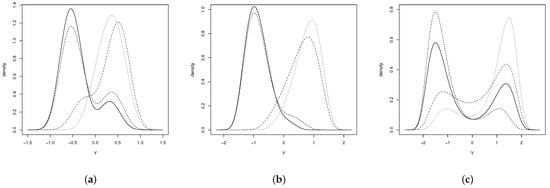
Figure 2. EGSHN distribution (a) $ESHN(0.75,0,1,3.5,-0.75)$ (solid line), $ESHN(0.75,0,1,2.5,-0.5)$ (dashed line), $ESHN(0.75,0,1,0.5,1.5)$ (dotted line) and $ESHN(0.75,0,1,1.5,0.75)$ (dash-dotted line), (b) $ESHN(1.5,0,1,3.5,-2.5)$ (solid line), $ESHN(1.5,0,1,2.5,-1.5)$ (dashed line), $ESHN(1.5,0,1,1.5,2.5)$ (dotted line) and $ESHN(1.5,0,1,0.5,1.5)$ (dash-dotted line) and (c) $ESHN(2.5,0,1,3.5,-0.25)$ (solid line), $ESHN(2.5,0,1,3.5,-0.75)$ (dashed line), $ESHN(2.5,0,1,2.5,0.75)$ (dotted line) and $ESHN(2.5,0,1,0.75,0.25)$ (dash-dotted line).

Likewise, for $\gamma =0$, we obtain the asymmetric SHN distribution based on the model considered by Leiva et al. (2010) [4]. In addition, if $\gamma \to \infty$, analogously to the ESHN case, we have the new family of distributions $g\left(y\right)\to 2b_y^2{b}_y^{\prime }\varphi \left(b_y\right)\mathsf{\Phi }\left(\lambda b_y\right).$ Now, for $\gamma =\lambda =0$, an SHN model is followed. It can also be shown that a random variable

$$b_Y=\frac{2}{\alpha }sinh\left(\frac{Y-\xi }{\sigma }\right)\sim ESN,$$

where $ESN$ is the extended skew-normal distribution, which was introduced by Elal-Olivero et al. (2009) [25]. As in the ESHN model, it can be shown that when $\alpha \to 0,$ then $g\left(y\right)\sim ESN.$

For p, as in the case of the ESHN model, the pdf of the $EGSHN(\alpha ,\xi ,\sigma ,\gamma ,\lambda )$ distribution could be written as

$$f\left(y\right)=2p{b}_y^{\prime }\varphi \left(b_y\right)\mathsf{\Phi }\left(\lambda b_y\right)+2(1-p)b_y^2{b}_y^{\prime }\varphi \left(b_y\right)\mathsf{\Phi }\left(\lambda b_y\right).$$

(18)

From (18), it follows that the cdf of $EGSHN(\alpha ,\xi ,\sigma ,\gamma ,\lambda )$ is given by

$$\begin{array}{c}\hfill F\left(y\right)={\mathsf{\Phi }}_{SN}(b_y;\lambda )-\frac{\gamma }{1+\gamma }{b}_y{\varphi }_{SN}(b_y;\lambda ),\end{array}$$

(19)

where $\mathsf{\Phi }(·;\lambda )$ and $\varphi (·;\lambda )$ denote the cdf and pdf of the skew-normal distribution, respectively, with a location parameter of 0 and a scale parameter of 1.

Then, the survival, risk (or hazard), and inverse risk functions of this distribution are, respectively, given by

$$h_G\left(t\right)=\frac{(1+\gamma b_t^2)h_{SSHN}\left(t\right)}{(1+\gamma )+\sigma \gamma tanh\left(z\right)h_{SSHN}\left(t\right)},\mathrm{and}{R}_G\left(t\right)=\frac{(1+\gamma b_t^2)R_{SSHN}\left(t\right)}{(1+\gamma )-\sigma \gamma tanh\left(z\right)R_{SSHN}\left(t\right)},$$

where $S_{SSHN},$ $h_{SSHN}\left(t\right),$ and $R_{SSHN}\left(t\right)$ are the survival, hazard, and inverse risk functions of the skew-SHN function, $SSHN(\alpha ,\xi ,\sigma ,\lambda ),$ respectively.

4.1. Stochastic Representation

The stochastic representation of the EGSHN model is based on Elal-Olivero (2010) [18] and Elal-Olivero, et al. (2009) [25]. This is presented below.

Definition 1.

If the random variable X has a pdf given by

$$r\left(x\right)=x^2\varphi \left(x\right),$$

then we say that X follows a bimodal-normal distribution, and it is denoted as $X\sim NB$ (see [18]).

Remark 1.

Let W and U independent random variables with $W\sim {\chi }_{\left(3\right)}^2$, a chi-square distribution with three degrees of freedom, and U a pdf, such that $P(U=-1)=P(U=1)=\frac{1}{2}$. If $Y=\sqrt{W}U$ then $Y\sim NB$.

Remark 2.

Let $Y\sim NB$ and considers the random variable $X_2$ which is defined as

$$X_2=\mathrm{arcsinh}(\alpha Y/2),$$

then,

$$\begin{array}{ccc}\hfill F_{X_2}\left(x\right)=P(X_2\le x)& =& P\left(\mathrm{arcsinh}(\alpha Y/2)\le x\right)\hfill \\ & =& P\left(Y\le \frac{2}{\alpha }sinh\left(x\right)\right)\hfill \\ & =& F_Y\left(\frac{2}{\alpha }sinh\left(x\right)\right).\hfill \end{array}$$

Then,

$$\begin{array}{ccc}\hfill f_{X_2}\left(x\right)& =& r\left(\frac{2}{\alpha }sinh\left(x\right)\right)\frac{2}{\alpha }cosh\left(x\right)\hfill \\ & =& {\left(\frac{2}{\alpha }sinh\left(x\right)\right)}^2\varphi \left(\frac{2}{\alpha }sinh\left(x\right)\right)\frac{2}{\alpha }cosh\left(x\right),\hfill \end{array}$$

which is denoted as $X_2\sim {\left(\frac{2}{\alpha }sinh\left(x\right)\right)}^2\varphi \left(\frac{2}{\alpha }sinh\left(x\right)\right)\frac{2}{\alpha }cosh\left(x\right)$.

Proposition 1.

Let $X_1\sim SHN(\alpha ,0,1)=SHN\left(\alpha \right)$ and $X_2\sim {\left(\frac{2}{\alpha }sinh\left(x\right)\right)}^2\varphi \left(\frac{2}{\alpha }sinh\left(x\right)\right)$ $\frac{2}{\alpha }\cosh \left(x\right)$, and say that $U\sim U(0,1)$ is a uniform random variable, independent of $X_1$ and $X_2.$ If

$$X=\left\{\begin{array}{cc}{X}_1,\hfill & \mathrm{if}U<\frac{1}{1+\gamma },\hfill \\ X_2,\hfill & \mathrm{if}U\ge \frac{\gamma }{1+\gamma },\hfill \end{array}\right.$$

with $\gamma >0,$ then $X\sim ESHN(\alpha ,\gamma )$.

Proof. 

$$\begin{array}{ccc}\hfill F_X\left(x\right)& =& P(X\le x)\hfill \\ & =& P\left(X\le x|U<\frac{1}{1+\gamma }\right)P\left(U<\frac{1}{1+\gamma }\right)+P\left(X\le x|U\ge \frac{1}{1+\gamma }\right)P\left(U\ge \frac{\gamma }{1+\gamma }\right)\hfill \\ & =& P(X\le x)\frac{1}{1+\gamma }+P(X\le x)\frac{\gamma }{1+\gamma }\hfill \\ & =& \frac{1}{1+\gamma }{F}_{X_1}\left(x\right)+\frac{\gamma }{1+\gamma }{F}_{X_2}\left(x\right),\hfill \end{array}$$

so

$$\begin{array}{ccc}\hfill f_X\left(x\right)& =& \frac{1}{1+\gamma }{f}_{X_1}\left(x\right)+\frac{\gamma }{1+\gamma }{f}_{X_2}\left(x\right)\hfill \\ & =& \frac{1+\gamma {\left(\frac{2}{\alpha }sinh\left(x\right)\right)}^2}{1+\gamma }\varphi \left(\frac{2}{\alpha }sinh\left(x\right)\right)\frac{2}{\alpha }\cosh \left(x\right).\hfill \end{array}$$

 □

Definition 2.

If the random variable W has a pdf

$$m\left(x\right)=2f\left(x\right)\mathsf{\Phi }\left(\lambda \frac{2}{\alpha }sinh\left(x\right)\right),x\in \mathbb{R},$$

with $\lambda \in \mathbb{R},$ then W follows a $EGSHN(\alpha ,\gamma ,\lambda )$ and this is denoted as $W\sim EGSHN(\alpha ,\gamma ,\lambda )$.

Proposition 2.

Let Z and X be independent random variables with $Z\sim N(0,1)$ and $X\sim ESHN$ $(\alpha ,\gamma )$.

If

$$W=\left\{\begin{array}{cc}X,\hfill & \mathrm{if}Z<\lambda \frac{2}{\alpha }sinh\left(x\right),\hfill \\ -X,\hfill & \mathrm{if}Z\ge \lambda \frac{2}{\alpha }sinh\left(x\right),\hfill \end{array}\right.$$

then $W\sim GESHN(\alpha ,\gamma ,\lambda )$.

Proof. 

Note that $W\left(X\right)=\lambda \frac{2}{\alpha }sinh\left(X\right)$ is an odd function and the density of both the random variables $-X$ and the distribution function of Z are symmetric around zero; thus, applying Lemma 1 as in [24], the result follows. □

Location-Scale Extension

Let $W\sim EGSHN(\alpha ,\gamma ,\lambda )$ and let $V=\mu +\sigma W,$ then

$$F_V\left(v\right)=P(V\le v)=P\left(\frac{v-\mu }{\sigma }\right)=F_W\left(\frac{v-\mu }{\sigma }\right).$$

Then, the pdf of V is given by

$$f_V\left(v\right)=\frac{1}{\sigma }{f}_W\left(\frac{v-\mu }{\sigma }\right)=\frac{2}{\sigma }f\left(\frac{v-\mu }{\sigma }\right)\mathsf{\Phi }\left(\lambda \frac{2}{\alpha }sinh\left(\frac{v-\mu }{\sigma }\right)\right),$$

which is denoted by $V\sim EGSHN(\alpha ,\mu ,\sigma ,\gamma ,\lambda ).$

4.2. Moments of an Extended Generalized Sinh-Normal Random Variable

For a random variable $Y\sim EGSHN(\alpha ,\xi ,\sigma ,\gamma ,\lambda )$, the r-th moment is given by

$$\mathbb{E}\left(Y^r\right)=\frac{1}{1+\gamma }\sum _{k=0}^r\left(\genfrac{}{}{0pt}{}{r}{k}\right){\sigma }^k{\xi }^{r-k}\left(d_{k0}(\alpha ,\lambda )+\gamma d_{k2}(\alpha ,\lambda )\right),$$

(20)

where

$$d_{kl}\left(\alpha \right)=2{\int }_{-\infty }^{\infty }{\left({sinh}^{-1}\left(\frac{\alpha }{2}w\right)\right)}^k{w}^l\varphi \left(w\right)\mathsf{\Phi }\left(\lambda w\right)dw.$$

(21)

4.3. Extended Generalized Birnbaum–Saunders Distribution

Let $Y\sim EGSHN(\alpha ,\xi ,2,\gamma ,\lambda ).$ Then, the distribution of a random variable $T=exp\left(Y\right)$ follows an extended generalized BS distribution, which is denoted by $EGBS(\alpha ,\beta ,\gamma ,\lambda )$, where $\beta =exp\left(\xi \right).$ The proof of this result is obtained from the transformation theorem of random variables. The pdf of an $EGBS(\alpha ,\beta ,\gamma ,\lambda )$ random variable is given by

$$\phi \left(t\right)=2\frac{1+\gamma a_t^2}{1+\gamma }{a}_t^{\prime }\varphi \left(a_t\right)\mathsf{\Phi }\left(\lambda a_t\right),$$

(22)

where $a_t=a_t(\alpha ,\beta )$ and $a_t^{\prime }=a_t^{\prime }(\alpha ,\beta )$ are defined as in (6).

Note that, for $\gamma =0$, we have the doubly generalized BS distribution developed by Vilca et al. (2006) [10] for the special case of the skew-normal distribution introduced by Azzalini (1985) [26], BSSN. If $\gamma \to \infty$, then $g\left(y\right)\to 2a_t^2{a}_t^{\prime }\varphi \left(a_t\right)\mathsf{\Phi }\left(\lambda a_t\right);$ if $\lambda =0$, then $\phi \left(t\right)$ follows the extended BS distribution class studied by Cortés et al. (2018) [17], and for $\gamma =\lambda =0$, $\phi \left(t\right)$ follows a BS model. Likewise, it can be shown that a random variable $a_T\sim ESN.$

As in the EGSHN model, it can be shown that the cdf of the $EGBS(\alpha ,\beta ,\gamma ,\lambda )$ distribution is given by

$$\begin{array}{c}\hfill F\left(y\right)={\mathsf{\Phi }}_{SN}(a_t;\lambda )-\frac{\gamma }{1+\gamma }{a}_t{\varphi }_{SN}(a_t;\lambda ).\end{array}$$

(23)

Then, the survival, risk, or hazard, and inverse risk functions of this distribution are given, respectively, by

$$S_{EGBS}\left(t\right)=S_{BSSN}\left(t\right)+\frac{\gamma }{1+\gamma }{a}_t{\varphi }_{SN}(a_t;\lambda ),$$

and

$$h_{EGBS}\left(t\right)=\frac{(1+\gamma a_t^2)(t+\beta )h_{BSSN}\left(t\right)}{(1+\gamma )(t+\beta )+{\beta }^{1/2}\gamma t(t-\beta )h_{BSSN}\left(t\right)}\mathrm{and}$$

$$R_{EGBS}\left(t\right)=\frac{(1+\gamma a_t^2)(t+\beta )R_{BSSN}\left(t\right)}{(1+\gamma )(t+\beta )-{\beta }^{1/2}\gamma t(t-\beta )R_{BSSN}\left(t\right)},$$

where $S_{BSSN},$ $h_{BSSN}\left(t\right)$ e $R_{BSSN}\left(t\right)$ are the survival, hazard, and inverse risk functions of the BS skew-normal model, $BSSN(\alpha ,\beta ,\lambda ).$ For the BSSN model, $li{m}_{t\to \infty }{h}_{BSSN}\left(t\right)=\frac{1+{\lambda }^2}{2{\alpha }^2\beta }$; then, for the EGBS model, it follows that $li{m}_{t\to \infty }{h}_{EGBS}\left(t\right)=0.$

Some properties of the BS model remain true for the EGBS model. Thus, if $T\sim EGBS(\alpha ,\beta ,\gamma ,\lambda )$, then (i) $aT\sim EGBS(\alpha ,a\beta ,\gamma ,\lambda )$, with $a>0$, and (ii) $T^{-1}\sim EGBS(\alpha ,{\beta }^{-1},$ $\gamma ,-\lambda )$.

The moments of an EGBS random variable with parameters $\alpha ,\beta ,\gamma ,$ and $\lambda$ can be obtained by means of the following expression:

$$\begin{array}{c}\hfill \mathbb{E}\left(T^r\right)=\frac{1}{{\alpha }^2\beta (1+\gamma )}\left[\gamma {\beta }^2{\mathbb{E}}_{BSSN}\left(T^{r-1}\right)+({\alpha }^2-2\gamma ){\mathbb{E}}_{BSSN}\left(T^r\right)+\gamma {\mathbb{E}}_{BSSN}\left(T^{r+1}\right)\right],\end{array}$$

(24)

where ${\mathbb{E}}_{BSSN}(·)$ is the expectation operator of the Birnbaum–Saunders skew-normal distribution (BSSN). To calculate the mean, variance, and the skewness and kurtosis coefficients of the EGBS model, the expressions of the corollaries 2.1 and 2.2 of Vilca et al. [10] could be used.

For $(\alpha ,\beta ,\gamma ,\lambda )$, the log-likelihood function corresponding to the random sample $t_1,t_2,\dots ,t_n$ is

$$\begin{array}{cc}\hfill \ell (\alpha ,\beta ,\gamma ,\lambda )=& \sum _{i=1}^{n}log\left(1+\gamma a_{t_i}^2\right)-nlog\left(1+\gamma \right)+\sum _{i=1}^{n}log\left(A_{t_i}\right)-\hfill \\ \hfill & \frac{1}{2}\sum _{i=1}^n{a}_{t_i}^2+\sum _{i=1}^{n}log\left(\mathsf{\Phi }\left(\lambda a_{t_i}\right)\right).\hfill \end{array}$$

(25)

The score function is composed of the following elements:

$$\begin{array}{cc}\hfill U\left(\alpha \right)=& -\frac{2\gamma }{\alpha }\sum _{i=1}^n\frac{a_{t_i}^2}{1+\gamma a_{t_i}^2}-\frac{1}{\alpha }\sum _{i=1}^n\left[1-a_{t_i}^2+\lambda a_{t_i}{\zeta }_i\right]=0,\hfill \end{array}$$

$$\begin{array}{cc}\hfill U\left(\beta \right)& =\frac{\gamma }{{\alpha }^2}\sum _{i=1}^n\frac{\frac{1}{t_i}-\frac{t_i}{{\beta }^2}}{1+\gamma a_{t_i}^2}-\frac{n}{2\beta }+\sum _{i=1}^n\frac{1}{\beta +t_i}-\frac{1}{2{\alpha }^2}\sum _{i=1}^n\left[\frac{1}{t_i}-\frac{t_i}{{\beta }^2}\right]\hfill \\ \hfill & -\frac{\lambda }{2\alpha {\beta }^{\frac{3}{2}}}\sum _{i=1}^n\frac{t_i+\beta }{t_i^{\frac{1}{2}}}{\zeta }_i=0,\hfill \end{array}$$

$$\begin{array}{c}\hfill U\left(\gamma \right)=-\frac{n}{1+\gamma }+\sum _{i=1}^n\frac{a_{t_i}^2}{1+\gamma a_{t_i}^2}=0,\end{array}\mathrm{and}\begin{array}{c}\hfill U\left(\lambda \right)=\sum _{i=1}^n{a}_{t_i}{\zeta }_i=0,\end{array}$$

where ${\zeta }_i=\frac{\varphi \left(\lambda a_{t_i}\right)}{\mathsf{\Phi }\left(\lambda a_{t_i}\right)}$, with $i=1,\dots ,n.$ Iterative numerical methods must be used to solve this system of nonlinear equations.

5. Extended Sinh-Normal Regression Model

One of our main goals is to develop a log-BS regression model based on the $ESHN(\alpha ,\xi ,$ $\sigma ,\gamma ,\lambda )$ model. This regression model will be an optimal alternative to the log-BS model introduced by Rieck et al. (1991) [3] in order to fit bimodal or survival asymmetric data. Now, the extended generalized log-linear BS regression model is defined following the considerations given by Rieck et al. (1991) [3] and considering that $Y_i$ is a dependent variable; that a set (p) of explanatory variables, denoted by ${\mathbf{x}}_i={(x_{i1},x_{i2},\cdots ,x_{ip})}^{\top }$, is given; and that $\mathit{\theta }=({\theta }_1,{\theta }_2,\dots ,{\theta }_p)$ is a p-dimensional vector of unknown parameters, where a linear predictor, ${\xi }_i={\mathbf{x}}_i^{\top }\mathit{\theta }$, is obtained for $i=1,2,\dots ,n$.

Then, let us suppose that $T_1,T_2,...T_n$ are independent and identically distributed random variables (i.i.d. r.v.) such that $T_i\sim \mathit{EGBS}({\alpha }_i,{\beta }_i,{\gamma }_i,{\lambda }_i)$. Now, let us suppose that the distribution of $T_i$ is independent of the set of explanatory variables, $x_i={(x_{i1},x_{i2},\dots ,x_{ip})}^{\prime }$, where

• ${\beta }_i=exp\left(x_i^{\prime }\mathbf{\theta }\right),$ for $i=1,2,\dots ,n,$ with ${\mathbf{\theta }}^{\prime }=({\theta }_1,{\theta }_2,...,{\theta }_p),$ being a p-dimensional vector of unknown parameters.
• The shape, bimodality, and skew parameters do not consider $x_i;$ i.e., ${\alpha }_i=\alpha ,{\gamma }_i=\gamma ,\mathrm{and}{\lambda }_i=\lambda \mathrm{for}i=1,2,\dots ,n.$

Let us suppose that $Y_i=log\left(T_i\right).$ Then, the extended generalized log-linear BS regression model is defined as

$$y_i={\mathbf{x}}_i^{\top }\mathit{\theta }+{ϵ}_i,i=1,\dots ,n,$$

(26)

where ${ϵ}_i\sim EGSHN(\alpha ,0,2,\gamma ,\lambda )$, for $i=1,\dots ,n$ and $y_i$ is the log-survival for the i-th individual. This model is denoted by $MRESHN(\alpha ,\theta ,2,\gamma ,\lambda ).$ When $\gamma =\lambda =0$ it follows the log-BS regression model, $LBS(\alpha ,\theta ,2)$, of Rieck et al. [3]; i.e., the MRESHN model is more flexible than the log-BS model in terms of skewness and kurtosis.

When $\lambda =0,$ it follows that ${ϵ}_i\sim ESHN(\alpha ,0,2,\gamma )$, for $i=1,\dots ,n$; then, important results are obtained. Thus, we find that $\mathbb{E}\left({ϵ}_i\right)=0$ and $Var\left({ϵ}_i\right)=4c_{20}\left(\alpha \right)$; additionally, as the errors are independent random variables, then for $i\ne i^{\prime }$, it follows that $Cov({ϵ}_i,{ϵ}_{i^{\prime }})=0.$ Furthermore, considering that the explanatory variables are independent of the shape parameter, from the above results, it is therefore possible to conclude that $Y_i\sim ESHN(\alpha ,{\mathbf{x}}_i^{\top }\mathit{\theta },2,\gamma )$ for $i=1,\dots ,n;$ furthermore, like $ϵ=0$, it can be shown that $\mathbb{E}\left(Y_i\right)={\xi }_i={\mathbf{x}}_i^{\top }\mathit{\theta },$ so the linear estimators for $\theta$ can be derived from the ordinary least squares method, whose solution is given by

$${\widehat{\mathit{\theta }}}^{\ast }={\left({\mathbf{X}}^{\top }\mathbf{X}\right)}^{-1}{\mathbf{X}}^{\top }\mathbf{Y},$$

with covariance matrix

$$Cov({\widehat{\mathit{\theta }}}^{\ast })=4c_{20}\left(\alpha \right){\left({\mathbf{X}}^{\top }\mathbf{X}\right)}^{-1}.$$

So, a biased estimator for $c_2\left(\alpha \right)$ could be

$${\widehat{c}}_{20}\left(\alpha \right)=\frac{1}{4(n-p)}\sum _{i=1}^n(y_i-{\mathbf{x}}_i^{\top }\widehat{\mathit{\theta }}).$$

Now, the model provided in (26) is a linear regression model similar to the models of the theory of linear models, with the characteristic that the random component follows a $EGSHN(\alpha ,0,2,\gamma ,\lambda )$ distribution; that is, assume that these parameters are located around zero and have a scale parameter equal to 2. Then, the interpretation of their parameters, with relation to the observed variable Y, is given in the same manner as the linear regression model.

For the vector ${(\alpha ,{\mathit{\theta }}^{\top },\gamma ,\lambda )}^{\top }$, we find that the log-likelihood function corresponding to the random sample $y_1,y_2,\dots ,y_n$ is

$$\begin{array}{cc}\hfill \ell (\alpha ,{\mathit{\theta }}^{\top },\gamma ,\lambda )=& \sum _{i=1}^{n}log\left(1+\gamma {\xi }_{i2}^2\right)-nlog\left(1+\gamma \right)+\sum _{i=1}^{n}log\left({\xi }_{i1}\right)-\hfill \\ \hfill & \frac{1}{2}\sum _{i=1}^n{\xi }_{i2}^2+\sum _{i=1}^{n}log\left(\mathsf{\Phi }\left(\lambda {\xi }_{i2}\right)\right),\hfill \end{array}$$

(27)

where ${\xi }_{i1}=2{\alpha }^{-1}cosh\left(z_i\right)$ and ${\xi }_{i2}=2{\alpha }^{-1}sinh\left(z_i\right)$ with $z_i={\displaystyle \frac{y_i-{\mathbf{x}}_i^{\top }\mathit{\theta }}{2}}$, for $i=1,2,\dots ,n.$ The elements of the score function are given by

$$\begin{array}{c}\hfill U\left(\alpha \right)=-\frac{2\gamma }{\alpha }\sum _{i=1}^n\frac{{\xi }_{i2}^2}{1+\gamma {\xi }_{i2}^2}-\frac{n}{\alpha }+\frac{1}{\alpha }\sum _{i=1}^n{\xi }_{i2}^2-\frac{\lambda }{\alpha }\sum _{i=1}^n{w}_i{\xi }_{i2},\end{array}$$

$$\begin{array}{cc}\hfill U\left({\theta }_j\right)=& -\gamma \sum _{i=1}^n{x}_{ij}\frac{{\xi }_{i1}{\xi }_{i2}}{1+\gamma {\xi }_{i2}^2}+\frac{1}{2}\sum _{i=1}^n{x}_{ij}\left({\xi }_{i1}{\xi }_{i2}-\frac{{\xi }_{i2}}{{\xi }_{i1}}\right)-\hfill \\ \hfill & \frac{\lambda }{2}\sum _{i=1}^n{x}_{ij}{\xi }_{i1}{w}_i,j=1,2,\dots ,p,\hfill \end{array}$$

$$\begin{array}{c}\hfill U\left(\gamma \right)=-\frac{n}{1+\gamma }+\sum _{i=1}^n\frac{{\xi }_{i2}^2}{1+\gamma {\xi }_{i2}^2},\mathrm{and}\end{array}\begin{array}{c}\hfill U\left(\lambda \right)=\sum _{i=1}^n{\xi }_{i2}{w}_i,\end{array}$$

where $w_i=\frac{\varphi \left(\lambda {\xi }_{i2}\right)}{\mathsf{\Phi }\left(\lambda {\xi }_{i2}\right)},\mathrm{for}i=1,\dots ,n.$

The maximum likelihood estimator of ${\theta }_1$, ${\theta }_2,\dots ,{\theta }_p$; $\alpha ;$ $\gamma$; and $\lambda$ is the solution to equations $U\left({\theta }_j\right)=0$, for $j=1,2,\dots ,p$; $U\left(\alpha \right)=0;$ $U\left(\gamma \right)=0$; and $U\left(\lambda \right)=0$, respectively, which require iterative numerical methods.

The least squares estimator (${\widehat{\theta }}^{\ast }$) may be used to initialize the iterative numerical process for $\theta$, and with these initial values, we can calculate ${\widehat{\alpha }}^{\ast }=\sqrt{\frac{4}{n}{\sum }_{i=1}^n\left[{sinh}^2\left(\frac{y_i-{\mathbf{x}}_i^{{}^{\prime }}{\widehat{\theta }}^{\ast }}{2}\right)\right]}.$

The elements of the observed information matrix, defined as minus the second derivative of the log-likelihood function, are denoted by $I_{\alpha \alpha },$ $I_{\alpha \theta },$ $I_{\alpha \gamma },I_{\alpha \lambda }$ $I_{{\theta }_j{\theta }_k},I_{{\theta }_j\gamma },I_{{\theta }_j\lambda },I_{\gamma \gamma },$ and $I_{\lambda \lambda }$, and are, respectively, given by

$$\begin{array}{cc}\hfill I_{\alpha \alpha }=& -\frac{n}{{\alpha }^2}-\frac{2\gamma }{{\alpha }^2}\sum _{i=1}^n\frac{3{\xi }_{i2}^2+\gamma {\xi }_{i2}^4}{{(1+\gamma {\xi }_{i2}^2)}^2}+\frac{3}{{\alpha }^2}\sum _{i=1}^n{\xi }_{i2}^2+\hfill \\ \hfill & \frac{\lambda }{{\alpha }^2}\sum _{i=1}^n{w}_i{\xi }_{i2}\left[-2+\lambda {\xi }_{i2}(\lambda {\xi }_{i2}+w_i)\right],\hfill \end{array}$$

$$\begin{array}{cc}\hfill I_{\alpha {\theta }_j}=& -\frac{\gamma }{\alpha }\sum _{i=1}^n{x}_{ij}\frac{{\xi }_{i1}{\xi }_{i2}}{{(1+\gamma {\xi }_{i2}^2)}^2}+\frac{1}{\alpha }\sum _{i=1}^n{x}_{ij}{\xi }_{i1}{\xi }_{i2}+\hfill \\ \hfill & \frac{\lambda }{2\alpha }\sum _{i=1}^n{x}_{ij}{w}_i{\xi }_{i1}\left[-1+\lambda {\xi }_{i2}(\lambda {\xi }_{i2}+w_i)\right],\hfill \end{array}$$

$$\begin{array}{cc}\hfill I_{\alpha \gamma }& =\frac{2}{\alpha }\sum _{i=1}^n\frac{{\xi }_{i2}^2}{{(1+\gamma {\xi }_{i2}^2)}^2},\hfill \end{array}\begin{array}{cc}\hfill I_{\alpha \lambda }& =\frac{1}{\alpha }\sum _{i=1}^n{w}_i{\xi }_{i2}\left[1-\lambda {\xi }_{i2}(\lambda {\xi }_{i2}+w_i)\right],\hfill \end{array}$$

$$\begin{array}{cc}\hfill I_{{\theta }_j{\theta }_k}& =\frac{1}{4}\sum _{i=1}^n{x}_{ij}{x}_{ik}\left\{2{\xi }_{i2}^2+\frac{4}{{\alpha }^2}-1+\frac{{\xi }_{i2}^2}{{\xi }_{i2}^2+4/{\alpha }^2}\right\}\hfill \\ \hfill & +\frac{2\gamma }{{\alpha }^2}\sum _{i=1}^n{x}_{ij}{x}_{ik}\left\{\frac{1}{1+\gamma {\xi }_{i2}^2}+\frac{2\gamma \frac{{\alpha }^2}{4}{\xi }_{i2}^2\left(\frac{4}{{\alpha }^2}+{\xi }_{i2}^2\right)}{{(1+\gamma {\xi }_{i2}^2)}^2}\right\}\hfill \\ \hfill & +\frac{\lambda }{4}\sum _{i=1}^n{x}_{ij}{x}_{ik}{w}_i\left[-{\xi }_{i2}+\lambda {\xi }_{i1}^2(\lambda {\xi }_{i2}+w_i)\right],\hfill \end{array}$$

$$\begin{array}{c}\hfill I_{{\theta }_j\gamma }=\sum _{i=1}^n{x}_{ij}\frac{{\xi }_{i1}{\xi }_{i2}}{{(1+\gamma {\xi }_{i2}^2)}^2},\end{array}\begin{array}{cc}\hfill I_{{\theta }_j\lambda }& =\frac{1}{2}\sum _{i=1}^n{x}_{ij}{w}_i{\xi }_{i1}\left[1-\lambda {\xi }_{i2}(\lambda {\xi }_{i2}+w_i)\right],\hfill \end{array}$$

$$\begin{array}{c}\hfill I_{\gamma \lambda }=0,\mathrm{and}\end{array}\begin{array}{c}\hfill I_{\lambda \lambda }=\sum _{i=1}^n{\xi }_{i2}^2{w}_i(\lambda {\xi }_{i2}+w_i).\end{array}$$

The information matrix ($\mathsf{\Psi }$) could be estimated as the expected value of the elements of the observed information matrix, which must be calculated using numerical approximation methods. For $\lambda =0,$ the sub-matrix of vector $(\alpha ,\theta ,\gamma )$ of the information matrix has the following elements:

$$\begin{array}{c}\hfill {\psi }_{\alpha \alpha }=\frac{2n}{{\alpha }^2}\frac{1+4\gamma }{1+\gamma }-\frac{2n}{{\alpha }^2}\frac{\gamma q_2\left(\gamma \right)}{1+\gamma },\end{array}\begin{array}{c}\hfill {\psi }_{\alpha {\beta }_j}=-\frac{4\gamma a_1}{\alpha }\sum _{i=1}^n{x}_{ij},\end{array}\begin{array}{c}\hfill {\psi }_{\alpha \gamma }=\frac{2n}{\gamma \alpha }{q}_1\left(\gamma \right),\end{array}$$

$$\begin{array}{cc}\hfill {\psi }_{{\beta }_j{\beta }_l}& =\frac{1}{{\alpha }^2(1+\gamma )}\left[\gamma +\frac{1}{2}{\alpha }^2(1+3\gamma )+\left(\frac{4\gamma }{{\alpha }^2}-1\right)m\left(\alpha \right)\right]\sum _{i=1}^n{x}_{ij}{x}_{il}\hfill \\ \hfill & +\frac{\gamma }{{\alpha }^2(1+\gamma )}\left[2+{\alpha }^2\left(1+\frac{1}{\gamma }\left(\frac{4\gamma }{{\alpha }^2}-1\right)q_1\left(\gamma \right)\right)\right]\sum _{i=1}^n{x}_{ij}{x}_{il},\hfill \end{array}$$

$$\begin{array}{c}\hfill {\psi }_{{\beta }_j\gamma }=2a_1\sum _{i=1}^n{x}_{ij},\end{array}\begin{array}{c}\hfill {\psi }_{\gamma \gamma }=-\frac{n}{{(1+\gamma )}^2}+\frac{n}{1+\gamma }{q}_3\left(\gamma \right),\end{array}$$

where $a_1={\int }_{-\infty }^{\infty }\frac{z\sqrt{1+\frac{4}{{\alpha }^2}{z}^2}}{1+\gamma z_2}\varphi \left(z\right)dz,$ $q_1\left(\gamma \right)=1-{\left(\frac{\pi }{2\gamma }\right)}^{1/2}\left\{1-erf{\left(\frac{1}{2\gamma }\right)}^{1/2}\right\}exp\left(\frac{1}{2\gamma }\right),$ $q_2\left(\gamma \right)$ $=1+\frac{2}{\gamma }{q}_1,$ $q_3\left(\gamma \right)=1-\frac{1}{\gamma }{q}_1\left(\gamma \right)$ and $m\left(\alpha \right)={\left(\frac{\pi {\alpha }^2}{8}\right)}^{1/2}\left\{1-erf{\left(\frac{2}{{\alpha }^2}\right)}^{1/2}\right\}exp\left(\frac{2}{{\alpha }^2}\right),$ with $erf(·)$ the error function (see Prudnikov et al. [27]).

For $\gamma >0$, the determinant of the information sub-matrix is not equal to zero; that is, $\left|\mathsf{\Psi }(\alpha ,\mathit{\theta },\gamma )\right|\ne 0$. Thus, it is possible to conclude that the information matrix of the ESHN model is nonsingular. Likewise, for $\lambda =0$, we find that

$${\psi }_{{\theta }_j\lambda }=\frac{1}{\alpha \sqrt{8\pi }}\left[{\left(2\gamma \right)}^{1/2}{\mathbb{E}}_{G(\frac{3}{2},\frac{1}{2\gamma })}(4\gamma +{\alpha }^{2}U)+{\mathbb{E}}_{G(\frac{1}{2},\frac{1}{2\gamma })}(4\gamma +{\alpha }^{2}U)\right]\sum _{i=1}^n{x}_{ij},$$

$$\begin{array}{c}\hfill {\psi }_{\lambda \gamma }=0,\mathrm{and}\end{array}\begin{array}{c}\hfill {\psi }_{\lambda \lambda }=n\sqrt{\frac{2}{\pi }}\frac{1+3\gamma }{1+\gamma },\end{array}$$

where $\mathbb{E}(·)$ denotes the expected value function, and $G(a,b)$ is the gamma distribution with parameters a and b, respectively. The rows or columns of the information matrix of the parameters vector $(\alpha ,{\mathit{\theta }}^{\top },\gamma ,\lambda )$ of the regression model $MRESHN$ in the case of $\lambda =0$ are linearly independent, Therefore, the information matrix of this model is nonsingular, and its inverse is the variance–covariance matrix, $\mathsf{\Sigma }\left(\widehat{\alpha },\widehat{\mathit{\theta }},\widehat{\gamma },\widehat{\lambda }\right),$ of the estimator vector of maximum likelihood of the parameters vector; then, the estimated standard errors of the estimators are the square root of the matrix $\widehat{\mathsf{\Sigma }}\left(\widehat{\mathit{\alpha }},\widehat{\mathbf{\theta }},\widehat{\gamma },\widehat{\lambda }\right).$

Then, when $n\to \infty$, the approximation $N_{p+4}\left(\left(\alpha ,\mathit{\theta },\gamma ,\lambda \right),\frac{1}{n}\mathsf{\Sigma }\left(\alpha ,\mathit{\theta },\gamma ,\lambda \right)\right)$ might be used to obtain a confidence interval for the parameter ${\theta }_r,$ for $r=1,2,\cdots ,p$, which is given by ${\widehat{\theta }}_r\mp z_{1-\rho /2}\sqrt{\widehat{\sigma }\left({\widehat{\theta }}_r\right)},$ where $\widehat{\sigma }(.)$ corresponds to the r-th element of the diagonal of the sub-matrix $\widehat{\mathsf{\Sigma }}(\widehat{\mathbf{\theta }})$ and $z_{1-\delta /2}$ is quartile $100(\delta /2)$ of the standard normal distribution.

6. Simulation Study

A simulation study is presented to analyze the performance of the maximum likelihood estimation of the parameters of the $EGSHN(\alpha ,{\beta }_0,{\beta }_1,\gamma ,\lambda )$ regression model. In general, $m=5000$ simulations with $n=30,60,90,120$, and 500 were generated for different scenarios. So, the following model, with ${\beta }_0=2.25$ and ${\beta }_1=0.75$, is studied.

$$y_i={\beta }_0+{\beta }_1{x}_i+{ϵ}_i,i=1,2,\cdots ,n.$$

Note that, for $i=1,2,\cdots ,n,$ $x_i$ takes values of a uniform random variable $(0,1)$, $X\sim U(0,1),$ and $ϵ\sim EGSHN(\alpha ,0,2,\gamma ,\lambda ).$ The statistics of the empirical standard deviation (sd), relative bias (RB) and $\sqrt{MSE}$ for the EGSHN model are calculated.

The results for each studied scenario are described as follows.

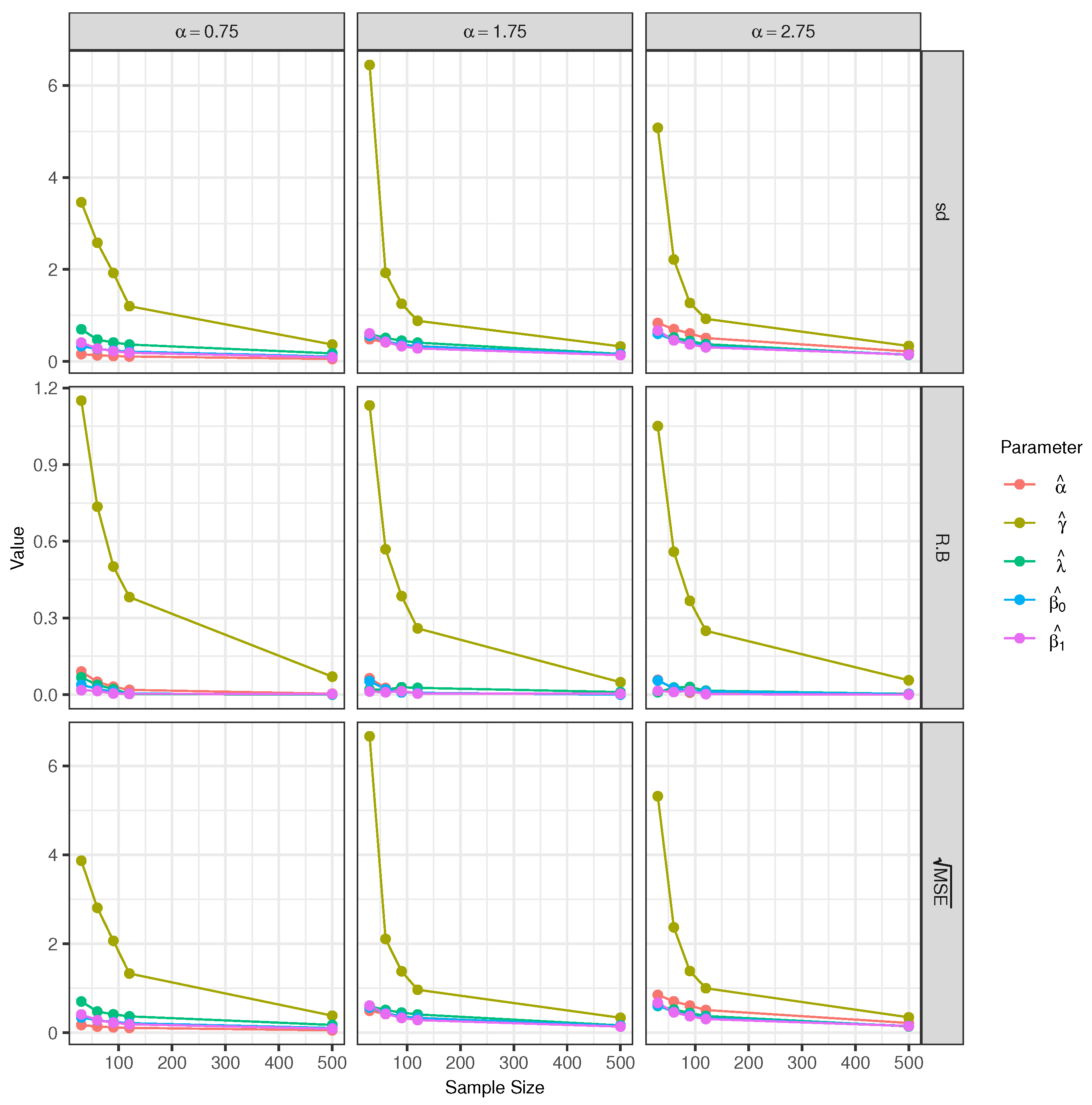
Scenario 1 (Varying α): In this scenario, the used alpha values are $0.75$, $1.75$, and $2.75$, keeping $\gamma =1.5$ and $\lambda =1$ fixed. For each studied case of the $EGSHN(\alpha ,2.25,0.75,1.5,1)$ model (see Figure 3 and Table 1), it can be seen that for the parameters ${\beta }_0$ and ${\beta }_1$, the relative biases are small, especially for the parameter ${\beta }_1$. Note that the statistics RB, sd, and $\sqrt{MSE}$ decrease when the sample size is increased.

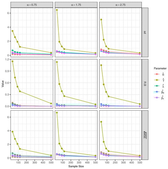
Figure 3. Empirical sd, relative bias, and $\sqrt{MSE}$ for the estimators of the $EGSHN(\alpha ,2.25,0.75,1.5,1)$ model parameters with sample sizes of 30, 60, 90, 120 and 500.

Table 1. Empirical sd, relative bias, and $\sqrt{MSE}$ for the $EGSHN(\alpha ,2.25,0.75,1.5,1)$ model.

		$\widehat{\mathit{\alpha }}$			$\widehat{\mathit{\gamma }}$			$\widehat{\mathit{\lambda }}$			${\widehat{\mathit{\beta }}}_0$			${\widehat{\mathit{\beta }}}_1$
$\mathit{\alpha }$	n	sd	RB	$\sqrt{\mathit{MSE}}$	sd	RB	$\sqrt{\mathit{MSE}}$	sd	RB	$\sqrt{\mathit{MSE}}$	sd	RB	$\sqrt{\mathit{MSE}}$	sd	RB	$\sqrt{\mathit{MSE}}$
	30	0.1600	0.0903	0.1737	3.4599	1.1505	3.8661	0.6997	0.0677	0.7029	0.3332	0.0386	0.3443	0.4105	0.0177	0.4107
	60	0.1339	0.0502	0.1390	2.5812	0.7354	2.8067	0.4756	0.0380	0.4770	0.2737	0.0226	0.2784	0.2818	0.0145	0.2819
0.75	90	0.1194	0.0311	0.1216	1.9235	0.5013	2.0651	0.4127	0.0216	0.4132	0.2396	0.0117	0.241	0.2252	0.0046	0.2252
	120	0.1087	0.0187	0.1096	1.2017	0.3818	1.3311	0.3681	0.0028	0.3681	0.2147	0.0040	0.2148	0.1897	0.0034	0.1897
	500	0.0541	0.0038	0.0542	0.3686	0.0705	0.3834	0.1759	0.0002	0.1759	0.1069	0.0017	0.1069	0.0913	0.0026	0.0913
	30	0.4831	0.0640	0.4958	6.4445	1.1316	6.6637	0.5962	0.0201	0.5965	0.5550	0.0531	0.5677	0.6102	0.0124	0.6102
	60	0.4162	0.0263	0.4187	1.9279	0.5686	2.1079	0.5113	0.0198	0.5116	0.4404	0.0211	0.4429	0.4255	0.0093	0.4255
1.75	90	0.3661	0.0135	0.3669	1.2541	0.3858	1.3811	0.4518	0.0292	0.4527	0.3657	0.0086	0.3662	0.3324	0.0137	0.3325
	120	0.3354	0.0063	0.3356	0.8840	0.2594	0.9657	0.4098	0.0267	0.4107	0.3303	0.0072	0.3307	0.2839	0.0040	0.2839
	500	0.1476	0.0012	0.1476	0.3285	0.0486	0.3364	0.1646	0.0101	0.1649	0.1568	0.0001	0.1568	0.1379	0.0036	0.1379
	30	0.8355	0.0578	0.8504	5.0777	1.0509	5.3163	0.6025	0.0095	0.6025	0.6021	0.0555	0.6149	0.6722	0.0149	0.6722
	60	0.7030	0.0225	0.7056	2.2156	0.5590	2.3687	0.5214	0.0280	0.5221	0.4612	0.0257	0.4648	0.4591	0.0102	0.4591
2.75	90	0.6090	0.0079	0.6094	1.2718	0.3672	1.3858	0.4443	0.0301	0.4452	0.3931	0.0139	0.3943	0.3725	0.0151	0.3727
	120	0.5096	0.0104	0.5104	0.9270	0.2499	0.9998	0.3758	0.0157	0.3761	0.3296	0.0127	0.3308	0.3076	0.0022	0.3075
	500	0.2182	0.0033	0.2184	0.3371	0.0563	0.3475	0.1417	0.0027	0.1417	0.1525	0.0022	0.1525	0.1496	0.0000	0.1496

Additionally, it can also be observed that the relative bias of the parameter $\alpha$ is not very important (not very large). Something similar is observed for the parameter $\lambda$. On the other hand, the relative bias and the root of the mean square error of the parameter $\gamma$ are not very small, especially when the sample size is small (30 or 60).

The statistics RB, sd, and $\sqrt{MSE}$ for the parameters $\alpha ,\gamma ,\lambda$ decrease when the sample size increases. These results guarantee a lack of bias and the asymptotic consistency of the estimates of the parameters $\alpha ,{\beta }_0,{\beta }_1,\gamma ,\lambda$.

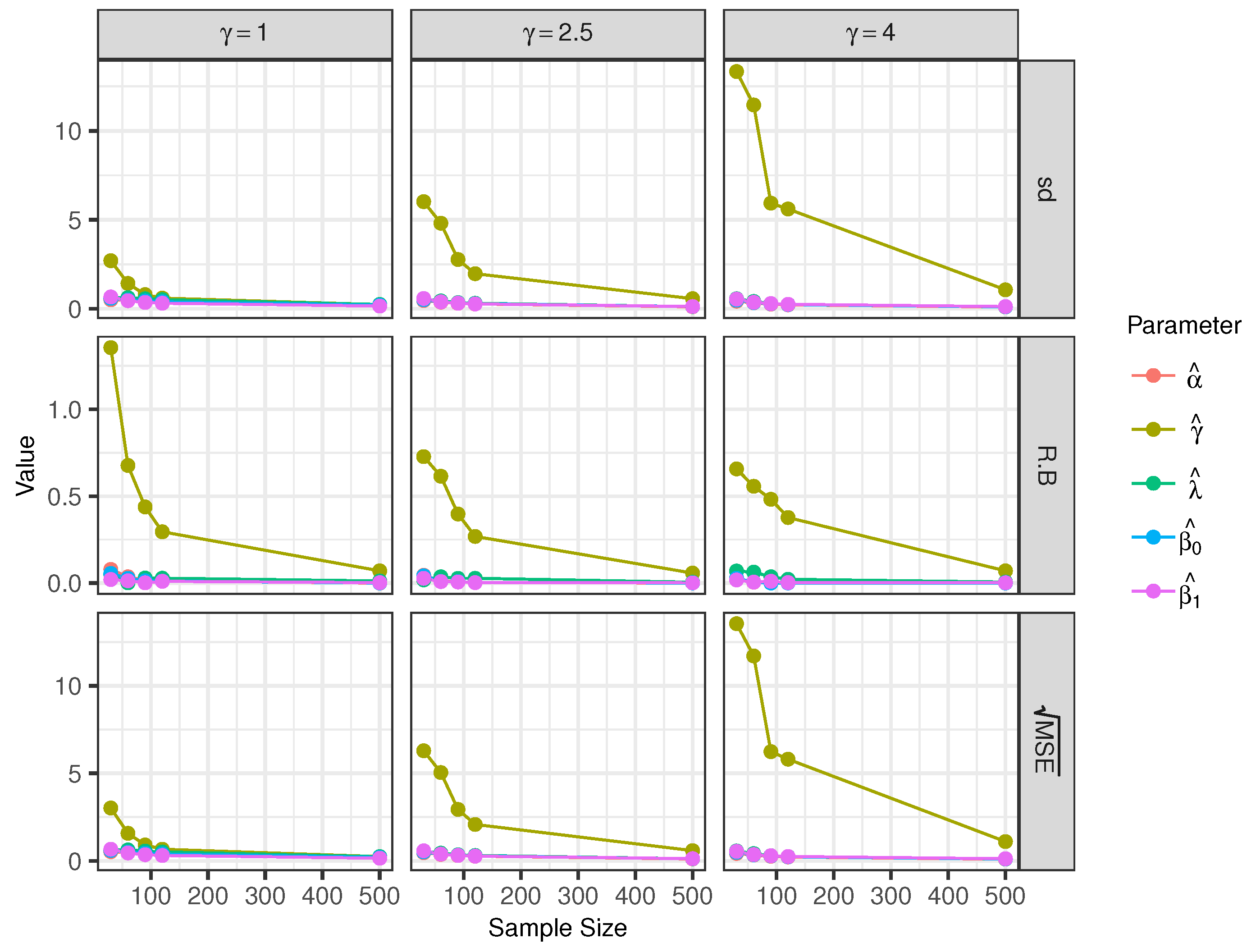
Scenario 2 (Varying γ): Here, the used gamma values are 1, 2.5, and 4, keeping $\alpha =1.75$ and $\lambda =1$ fixed. Similar to scenario 1, we can see that the parameters ${\beta }_0$ and ${\beta }_1$ present small relative biases (see Figure 4 and Table 2). The statistics RB, sd, and $\sqrt{MSE}$ of the $EGSHN(1.75,2.25,0.75,\gamma ,1)$ model decrease when the sample size is increased.

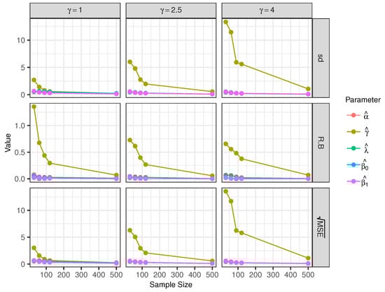
Figure 4. Empirical sd, relative bias, and $\sqrt{MSE}$ for the estimators of the $EGSHN(1.75,2.25,0.75,\gamma ,1)$ model parameters with sample sizes of 30, 60, 90, 120 and 500.

Table 2. Empirical sd, relative bias, and $\sqrt{MSE}$ for the $EGSHN(1.75,2.25,0.75,\gamma ,1)$ model.

		$\widehat{\mathit{\alpha }}$			$\widehat{\mathit{\gamma }}$			$\widehat{\mathit{\lambda }}$			${\widehat{\mathit{\beta }}}_0$			${\widehat{\mathit{\beta }}}_1$
$\mathit{\gamma }$	n	sd	RB	$\sqrt{\mathit{MSE}}$	sd	RB	$\sqrt{\mathit{MSE}}$	sd	RB	$\sqrt{\mathit{MSE}}$	sd	RB	$\sqrt{\mathit{MSE}}$	sd	RB	$\sqrt{\mathit{MSE}}$
	30	0.5060	0.0784	0.5242	2.6997	1.3552	3.0205	0.6351	0.0473	0.6368	0.5845	0.0553	0.5975	0.6630	0.0204	0.6631
	60	0.4768	0.0359	0.4809	1.4215	0.6769	1.5743	0.6234	0.0014	0.6233	0.4910	0.0272	0.4948	0.4506	0.0130	0.4507
1.0	90	0.4368	0.0159	0.4376	0.7941	0.4384	0.9071	0.5594	0.0290	0.5601	0.4321	0.0130	0.4330	0.3520	0.0017	0.3520
	120	0.3930	0.0121	0.3935	0.5962	0.2952	0.6652	0.5107	0.0281	0.5115	0.3900	0.0113	0.3908	0.3088	0.0100	0.3088
	500	0.1957	0.0000	0.1957	0.2305	0.0703	0.2409	0.2402	0.0121	0.2404	0.1977	0.0005	0.1977	0.1493	0.0026	0.1493
	30	0.4612	0.0446	0.4677	6.0222	0.7279	6.2906	0.5485	0.0185	0.5487	0.5092	0.0417	0.5178	0.5756	0.0272	0.5759
	60	0.3695	0.0123	0.3701	4.8084	0.6148	5.0476	0.4371	0.0360	0.4386	0.3835	0.0093	0.3841	0.3859	0.0084	0.3859
2.5	90	0.3035	0.0089	0.3039	2.7667	0.3974	2.9394	0.3429	0.0270	0.3439	0.3177	0.0083	0.3182	0.3121	0.0062	0.3121
	120	0.2655	0.0026	0.2655	1.9695	0.2684	2.0805	0.3056	0.0274	0.3068	0.2768	0.0029	0.2768	0.2694	0.0026	0.2690
	500	0.1129	0.0007	0.1129	0.5670	0.0575	0.5849	0.1213	0.0049	0.1214	0.1257	0.0008	0.1257	0.1270	0.0014	0.1270
	30	0.4246	0.0245	0.4267	13.3364	0.6570	13.5521	0.5613	0.0693	0.5655	0.4786	0.0269	0.4824	0.5404	0.0179	0.5406
	60	0.3298	0.0048	0.3298	11.4564	0.5569	11.7093	0.4094	0.0631	0.4142	0.3450	0.0060	0.3452	0.3628	0.0054	0.3628
4.0	90	0.2629	0.0015	0.2629	5.9366	0.4821	6.2414	0.2938	0.0363	0.2960	0.2792	0.0002	0.2792	0.2922	0.0103	0.2922
	120	0.2210	0.0018	0.2210	5.6103	0.3773	5.8091	0.2506	0.0218	0.2515	0.2328	0.0005	0.2328	0.2498	0.0027	0.2498
	500	0.0982	0.0007	0.0982	1.0651	0.0704	1.1016	0.1075	0.0057	0.1076	0.1111	0.0001	0.1111	0.1218	0.0018	0.1218

The parameters $\alpha$ and $\lambda$ show very small relative biases, but the parameter $\gamma$ presents large relative biases and $\sqrt{MSE}$. This behavior of the gamma parameter is more striking for small sample sizes.

The asymptotic consistency of the estimates of the parameters $\alpha ,{\beta }_0,{\beta }_1,\gamma ,\lambda$ can be guaranteed because the calculated statistics for $\alpha ,\gamma ,\lambda$ decrease when sample size increases.

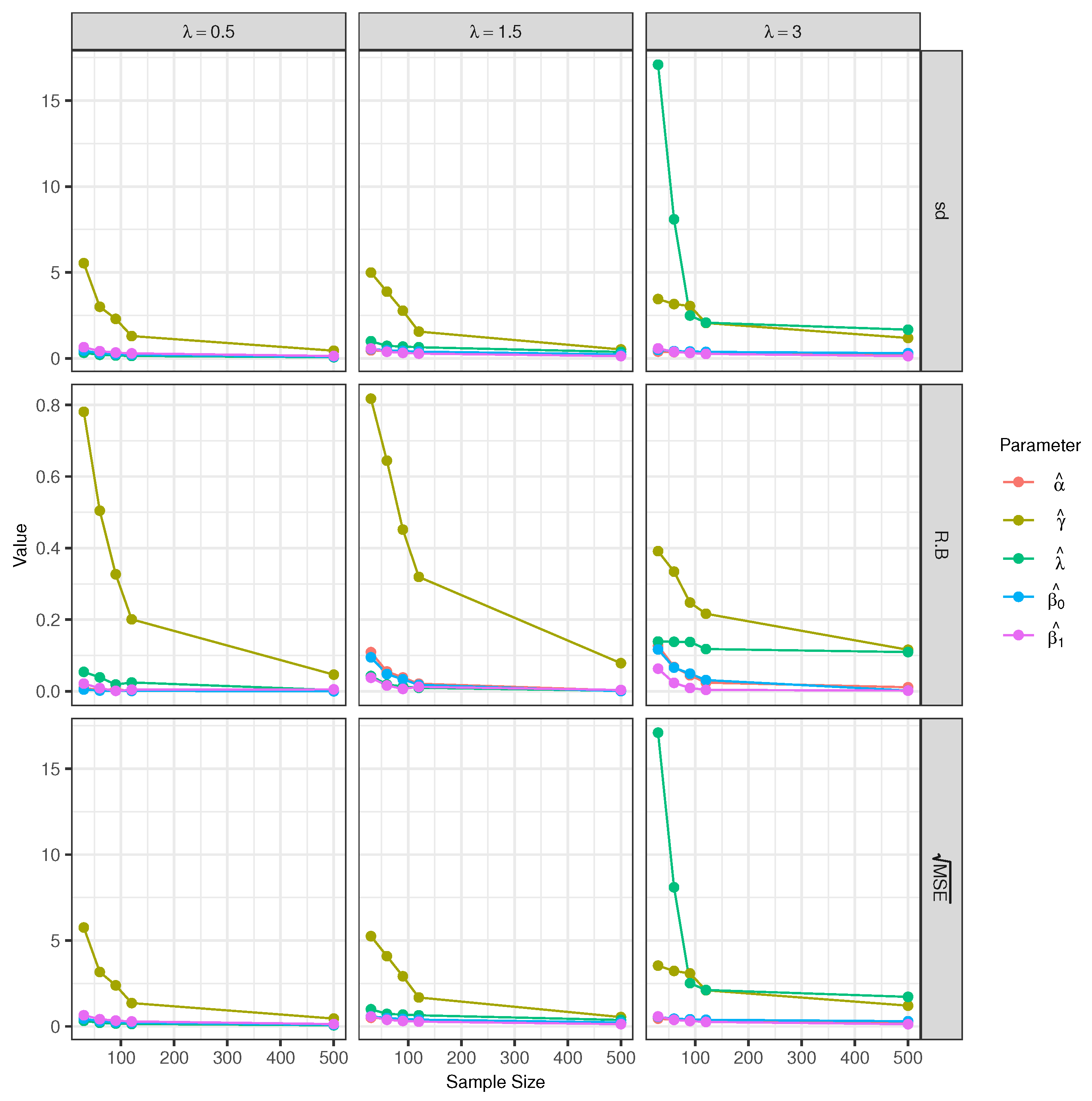
Scenario 3 (Varying λ): In scenario 3, where the $EGSHN(1.75,2.25,0.75,2,\lambda )$ model is considered, the used lambda values are $0.5$, $1.5$, and 3, keeping $\alpha =1.75$ and $\gamma =2$ fixed (see Figure 5 and Table 3). As in the previous simulation scenarios, the relative biases for the parameters ${\beta }_0$ and ${\beta }_1$ are small, especially for the parameter ${\beta }_1$. It is possible to see that the statistics RB, sd, and $\sqrt{MSE}$ tend to decrease when the sample size increase.

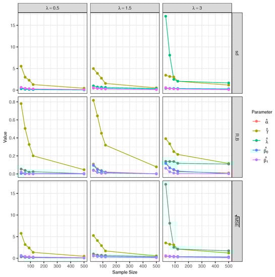
Figure 5. Empirical sd, relative bias, and $\sqrt{MSE}$ for the estimators of the $EGSHN$ $(1.75,2.25,0.75,2.0,\lambda )$ model parameters with sample sizes of 30, 60, 90, 120 and 500.

Table 3. Empirical sd, relative bias, and $\sqrt{MSE}$ for the $EGSHN(1.75,2.25,0.75,2.0,\lambda )$ model.

		$\widehat{\mathit{\alpha }}$			$\widehat{\mathit{\gamma }}$			$\widehat{\mathit{\lambda }}$			${\widehat{\mathit{\beta }}}_0$			${\widehat{\mathit{\beta }}}_1$
$\mathit{\lambda }$	n	sd	RB	$\sqrt{\mathit{MSE}}$	sd	RB	$\sqrt{\mathit{MSE}}$	sd	RB	$\sqrt{\mathit{MSE}}$	sd	RB	$\sqrt{\mathit{MSE}}$	sd	RB	$\sqrt{\mathit{MSE}}$
	30	0.3354	0.0083	0.3357	5.5409	0.7808	5.7563	0.3244	0.0541	0.3255	0.4508	0.0048	0.4509	0.6493	0.0215	0.6494
	60	0.2278	0.0042	0.2279	3.0014	0.5044	3.1661	0.2077	0.0389	0.2086	0.2991	0.0020	0.2991	0.4186	0.0087	0.4186
0.50	90	0.1779	0.0055	0.1782	2.2964	0.3269	2.3874	0.1637	0.0189	0.1640	0.2386	0.0014	0.2386	0.3376	0.0011	0.3376
	120	0.1570	0.0008	0.1570	1.2968	0.2010	1.3575	0.1412	0.0246	0.1417	0.2094	0.0011	0.2094	0.2892	0.0046	0.2890
	500	0.0711	0.0018	0.0711	0.4458	0.0465	0.4554	0.0639	0.0035	0.0639	0.0955	0.0000	0.0955	0.1374	0.0053	0.1374
	30	0.4651	0.1093	0.5029	4.9920	0.8175	5.2525	0.9968	0.0428	0.9988	0.5470	0.0949	0.5872	0.5720	0.0377	0.5727
	60	0.4308	0.0552	0.4414	3.8817	0.6443	4.0896	0.7276	0.0189	0.7276	0.4703	0.0479	0.4824	0.3853	0.0162	0.3855
1.5	90	0.4041	0.0385	0.4096	2.7730	0.4517	2.9162	0.6860	0.0133	0.6860	0.4268	0.0335	0.4333	0.3179	0.0066	0.3179
	120	0.3746	0.0211	0.3764	1.5575	0.3195	1.6834	0.6473	0.0097	0.6475	0.3894	0.0179	0.3915	0.2758	0.0123	0.2760
	500	0.2312	0.0024	0.2312	0.5188	0.0785	0.5420	0.3727	0.0013	0.3738	0.2313	0.0004	0.2313	0.1314	0.0037	0.1314
	30	0.3930	0.1271	0.4515	3.4510	0.3915	3.5384	17.0967	0.1390	17.0977	0.4872	0.1168	0.5535	0.5789	0.0631	0.5808
	60	0.3635	0.0677	0.3823	3.1596	0.3342	3.2292	8.0921	0.1382	8.0979	0.4215	0.0661	0.4469	0.3792	0.0234	0.3796
3.0	90	0.3421	0.0446	0.3508	3.0435	0.2479	3.0834	2.4923	0.1378	2.5170	0.4013	0.0493	0.4163	0.3132	0.0092	0.3133
	120	0.3237	0.0240	0.3264	2.0577	0.2166	2.1026	2.0773	0.1180	2.1181	0.3781	0.0313	0.3846	0.2592	0.0039	0.2592
	500	0.2590	0.0113	0.2597	1.1857	0.1159	1.208	1.6695	0.1095	1.7197	0.2996	0.0019	0.2996	0.1298	0.0018	0.1290

The RB and $\sqrt{MSE}$ of the parameter $\gamma$ are large for small sample sizes. The parameter $\alpha$ presents small relative biases, but the parameter $\lambda$ shows a large sd and $\sqrt{MSE}$ when $\lambda =3$. In general, we can see that the asymptotic consistency of the estimates of the parameters $\alpha ,{\beta }_0,{\beta }_1,\gamma ,\lambda$ is satisfied.

7. Numerical Illustrations

7.1. Illustration 1

In this paper, we employed the dataset studied by Hirose (1993) [28] to show the relevance of the EGSHN model. This dataset contains the results of an accelerated life test on polyethylene terephthalate (PET) (used in electrical isolation) in SF6 gas-insulated transformers. Such an accelerated life test was performed at four voltage levels (5, 7, 10, and 15), with 7, 15, 10, and 9 observations per level, respectively. The main purpose of the study was to analyze the resistance times (t) of the insulating films at different voltages (v). Hence, we here consider the following regression model:

$$y_i=log\left(t\right)={\beta }_0+{\beta }_1\ast v_i+{ϵ}_i,$$

where $y_i$ follows an $EGSHN(\alpha ,{\beta }_0+{\beta }_1\ast v_i,\sigma ,\gamma ,\lambda )$ distribution.

In this work, the SHN and ESHN models are fitted (see Ortega et al. [29]). To compare these models, the Akaike (AIC) information criterion (Akaike, [30]) and the corrected Akaike (AICC) criterion (Cavanaugh, [31]) are implemented. These measures are defined as follows:

$$AIC=-2\ell (\widehat{\theta })+2p\mathrm{and}AICC=-2\ell (\widehat{\theta })+\frac{2n(p+1)}{n-p-2},$$

where p is the number of parameters and $\widehat{\ell }(·)$ is the log-likelihood function evaluated for the MLEs of parameters. The best model is that with the smallest AIC or AICC value. To fit the bivariate model, we used the optim function of the statistical package R Core Team.

The estimated parameters of these models, accompanied by their standard errors in parentheses, are obtained using the maximum likelihood method. Table 4, shows the results. Note that according to the AIC and AICC, the EGSHN and ESHN models present the best fits.

Table 4. Estimated parameters, with their standard errors for the SHN, ESHN, and EGSHN models.

Estimator	SHN	ESHN	EGSHN
$\widehat{\alpha }$	245.9799	66.9952	7.9489
	(230.85)	(48.8845)	(2.6274)
${\widehat{\beta }}_0$	9.2750	9.3422	9.3456
	(0.1595)	(0.1666)	(0.1616)
${\widehat{\beta }}_1$	−0.4217	−0.4077	−0.4144
	(0.0190)	(0.0165)	(0.0189)
$\widehat{\sigma }$	0.3572	0.4306	0.7539
	(0.0536)	(0.0585)	(0.0903)
$\widehat{\gamma }$		0.3070	6.1671
		(0.1166)	(3.3568)
$\widehat{\lambda }$			−0.6493
			(0.1965)
AIC	89.59	74.42	73.1924
AICC	93.30	78.89	78.58

In order to identify atypical observations and/or the misspecifications of models, we analyzed the transformation of the martingale residual, rMTi, proposed by Barros et al. [8]. These residuals are defined by

$$rM{T}_i=sgn\left(r{M}_i\right)\sqrt{-2[r{M}_i+{\alpha }_{i}log({\alpha }_i-r{M}_i)]};\mathrm{for}i=1,2,3,\cdots ,n,$$

where $r{M}_i={\alpha }_i+log(S(e_i,\widehat{\theta }))$ is the martingale residual proposed by Ortega et al. [32], where ${\alpha }_i=0,1$ indicates whether the i-th observation is censored or not, respectively; $sgn\left(r{M}_i\right)$ denotes the sign of $r{M}_i$; and $S(e_i;\widehat{\theta })$ represents the survival function evaluated in $e_i$, where $\widehat{\theta }$ are the MLE for $\theta$.

The plots of $rM{T}_i$ with generated confidence envelopes is presented in Figure 6. From this figure, we can see clearly that the EGSHN model fits better to the data than the SHN and ESHN models, since, in these cases, there are no observations that lie outside the envelopes.

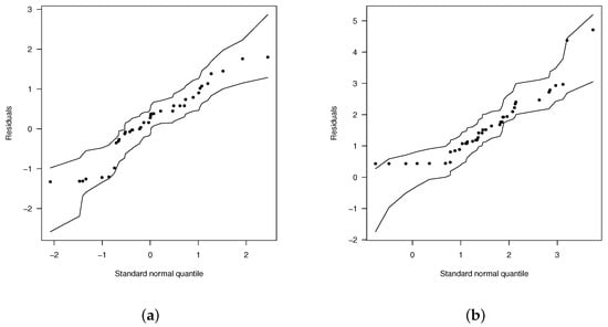
Figure 6. Normal probability plots for $rM{T}_i$ with envelopes of Q-qplots for the scaled residuals, from the fitted models. (a) ESHN and (b) EGSHN.

In Figure 6b, we observe two points: one in the border and the other outside it. There is also a point far from the set of observations. Since these points could be values influencing the estimates of the parameters, we calculated the generalized Cook’s distance (GCD) and showed the residual components of the deviation plot. Figure 7 illustrates the behavior of these two statistics. As can be seen in this figure, observations 8, 23, and 34 could be possible influential values. Thus, to calculate their impact on the estimates, we computed the estimates by eliminating each of these observations or groups of them.

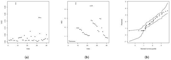
Figure 7. Influence measures for the EGSHN model (a) Cook’s distance, (b) $rM{T}_i$, (c) envelope picture of EGSHN model.

The relative change (RC), in percentage, of each parameter estimate is used to evaluate the effect of the potentially influential case. The RC is given by $RC\left({\theta }_{\left(i\right)}\right)=100\times |(\widehat{\theta }-{\widehat{\theta }}_{\left(i\right)})/\widehat{\theta }|$, where ${\widehat{\theta }}_{\left(i\right)}$ denotes the MLE of $\theta$ after removing the i-th observation. Table 5 lists the obtained RC values. According to this table, the relative changes of the MLE of parameter $\lambda$ are excessively pronounced in all the models, mainly for observation 8 and the $\{8,23\}$ set. Thus, after deleting observations 8 and 23, the new estimates of the parameter are $\widehat{\alpha }=8.5382\left(2.7109\right),$ ${\widehat{\beta }}_0=9.4767\left(0.1500\right),$ ${\widehat{\beta }}_1=-0.4311\left(0.0184\right),$ $\widehat{\sigma }=0.6937\left(0.0833\right),$ $\widehat{\gamma }=5.8458\left(3.0420\right),$ and $\widehat{\lambda }=-0.6106\left(0.1838\right),$ with $AIC=59.30$ and $AICC=64.91,$ as illustrated in Figure 7c.

Table 5. Relative change of the estimates of the EGSHN model.

Observation	$\widehat{\mathit{\alpha }}$	${\widehat{\mathit{\beta }}}_0$	${\widehat{\mathit{\beta }}}_1$	$\widehat{\mathit{\sigma }}$	$\widehat{\mathit{\gamma }}$	$\widehat{\mathit{\lambda }}$
8	0.0752	1.0751	3.6291	4.4136	0.2496	9.5977
23	0.1942	0.0200	0.2091	1.2090	0.0877	2.5542
34	0.2357	1.5518	4.3536	1.0540	0.3764	7.9936
8, 23	0.0839	0.8594	2.8812	5.7076	0.3233	13.8282
8, 34	0.0253	0.6924	2.0139	3.4098	0.1873	10.0372
23, 34	0.0731	0.9189	3.0378	0.6211	0.2350	8.8319
8, 23, 34	0.0326	0.6332	1.7068	5.2954	0.2438	14.2785

7.2. Illustration 2

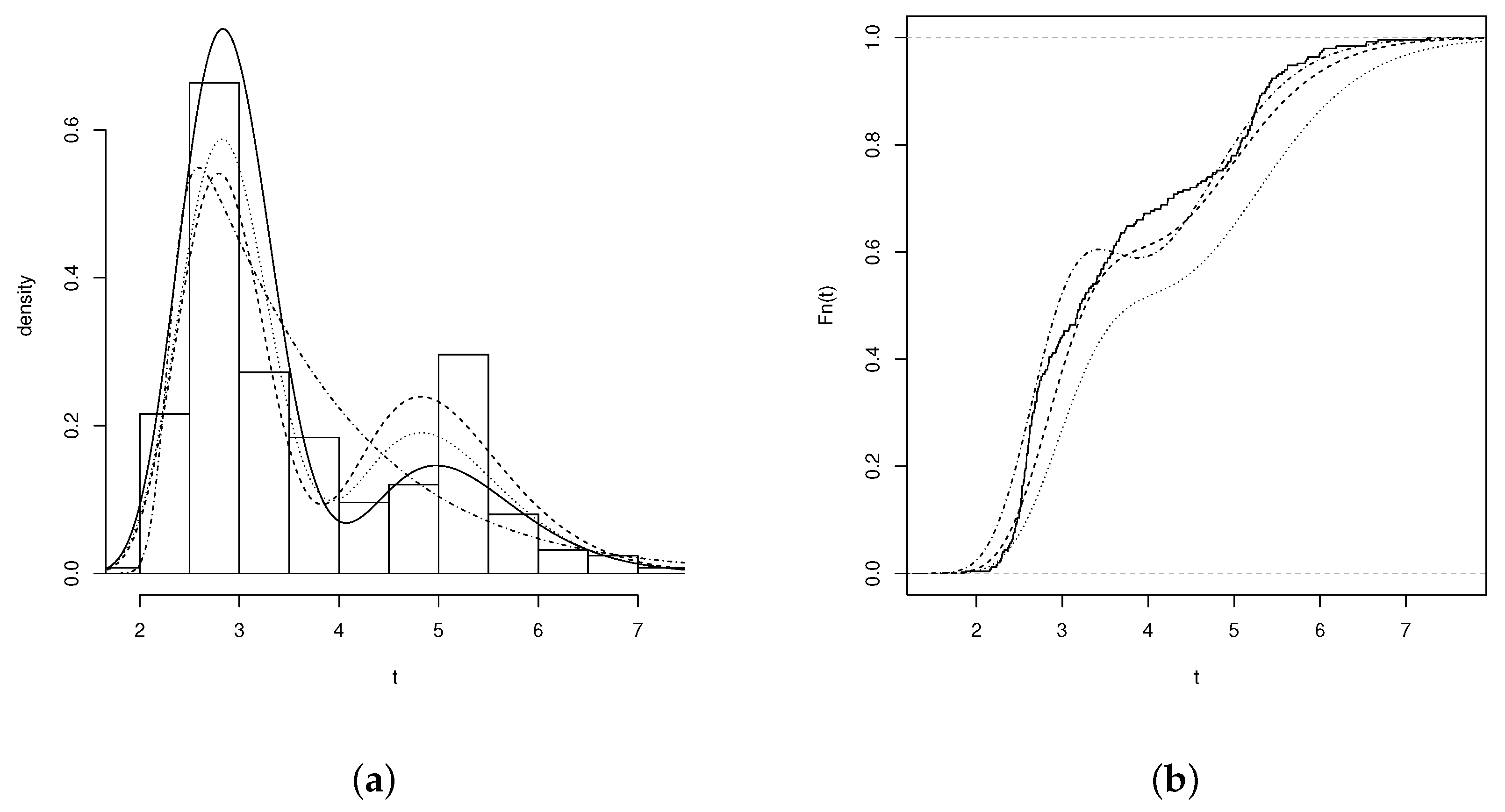
We used the dataset reported by the Center for Applied Statistics of the Institute of Mathematics and Statistics at the University of São Paulo to illustrate the relevance of the EGBSSN model. This dataset contains data on the amount of DNA within the nucleus (ploidy) of mammary cells (250 samples) from women with breast cancer. The ploidy variable exhibits a bimodal asymmetric performance, with D = 0.0399 and p-value = 0.0059 after performing the Hartigan and Hartigan (1985) [33] bimodality test. In addition, according to its descriptive statistics (presented in Table 6), this variable has a considerable positive skewness and high kurtosis. Additionally, Figure 8a shows a bimodal distribution of the data, which is why the EGBSSN model becomes an alternative to fit this kind of data.

Table 6. Descriptive statistics of the ploidy dataset.

$\overline{\mathit{y}}$	${\mathit{s}}_{\mathit{y}}^2$	$\sqrt{{\mathit{b}}_1}$	${\mathit{b}}_2$
3.636	1.432	0.452	0.865

Figure 8. (a) Histogram of the variable (amount of DNA in cancer cells) for the EGBS (solid line), EBS (dashed line), BLSN (dotted line), and BSSN (dash-dotted line) adjusted distributions; and (b) empirical cumulative distribution (solid line) and for the EGBS (dashed line), EBS (dotted line), and BLSN (dash-dotted line) models.

In this study, the Birnbaum–Saunders (BS) and Birnbaum–Saunders skew-normal models were fitted. We also considered the following bimodal models: the log-skew-normal model developed by Bolfarine et al. (2011) [16], the extended class (EBN) introduced by Cortez et al. (2018) [17], and the EGBS model.

Table 7 presents the maximum likelihood estimates and AIC and AICC values of five models. As observed in this table, the BS and BSSN models provide a poor fit to the DNA dataset. Conversely, the EGBS model shows the best fit among the fitted models, which is explained by its flexibility to fit asymmetric bimodal data.

Table 7. Estimated parameters (standard errors) for the fitted models.

Estimators	BS	BSSN	BLSN	EBS	EGBS
$\widehat{\alpha }$	(0.3145)	0.5254	1.3564	0.2033	0.2136
	(0.0140)	(0.0263)	(0.0169)	(0.0066)	(0.0082)
$\widehat{\beta }$	3.5194	2.3042	0.2066	3.7995	4.0200
	(0.0698)	(0.032)	(0.0070)	(0.0551)	(0.0643)
${\widehat{\gamma }}_1$			3.9845	4.4899	5.6760
			(1.2161)	(1.7541)	(2.5460)
$\widehat{\lambda }$		7.7814	−0.2874		−0.3724
		(1.2943)	(0.0677)		(0.0701)
AIC	745.58	698.51	671.95	668.41	637.8484
AICC	747.68	700.68	674.20	670.58	640.09

Figure 8a,b shows the estimated densities of the models with the best fit (BSSN, BLSN, EBS, and EGBS); the empirical cumulative distribution functions of the BLSN, EBS, and EGBS models; and the parameter estimates. Note that the EGBS model provides the best fit when compared to the BSSN, BLSN, EBN, and BS models.

8. Discussion

Bimodality and skewness are two common features that may be present in data from engineering, geo-spatial, medicine, and other areas. The natural complexity of data from these areas needs to be fitted using models that offer great flexibility and goodness of fit. In some cases, the data only present positive skewness, or in other cases, the distribution is only bimodal, but these two features could be present simultaneously. Thus, in this paper, a distribution capable of fitting bimodal and positively skewed data sets was proposed. In addition, the extended Birnbaum–Saunders distribution was studied as well.

Although there are proposals in the literature such as those cited in the previous sections, which allow the fitting of asymmetric or bimodal data, our model has the characteristic of modeling data that simultaneously have these two characteristics and has great flexibility and goodness of fit for data with these conditions. It is a new, promising, and user-friendly option to consider in statistical analysis.

To conclude, the EGBS model was proposed as a new statistical distribution suitable to fit real data sets with positive skewness and bimodality that presents a great performance compared with models available in the literature and that aim to achieve the same objective.

References

- Birnbaum, Z.W.; Saunders, S.C. A New Family of Life Distributions. J. Appl. Probab. 1969, 6, 319–327. [Google Scholar] [CrossRef]
- Desmond, A. Stochastic models of Failure in random environments. Can. J. Stat. 1985, 13, 171–183. [Google Scholar] [CrossRef]
- Rieck, J.R.; Nedelman, J.R. A log-linear model for the Birnbaum-Saunders distribution. Technometrics 1991, 33, 51–60. [Google Scholar]
- Leiva, V.; Vilca-Labra, F.; Balakrishnan, N.; Sanhueza, A. A skewed sinh-normal distribution and its properties and application to air pollution. Commun. Stat. Theory Methods 2010, 39, 426–443. [Google Scholar] [CrossRef]
- Lemonte, A.J. A log-Birnbaum-Saunders regression model with asymmetric errors. J. Stat. Comput. Simul. 2011, 82, 1775–1787. [Google Scholar] [CrossRef] [Green Version]
- Martínez-Flórez, G.; Bolfarine, H.; Gómez, H.W. The Log-Linear Birnbaum-Saunders Power Model. Methodol. Comput. Appl. Probab. 2017, 19, 913–933. [Google Scholar] [CrossRef]
- Moreno-Arenas, G.; Martínez-Flórez, G.; Barrera-Causil, C. Proportional Hazard Birnbaum-Saunders Distribution with Application to the Survival Data Analysis. Rev. Colomb. Estad. 2016, 39, 129–147. [Google Scholar] [CrossRef]
- Barros, M.; Galea, M.; Gonzalez, M.; Leiva, V. Influence diagnostics in the tobit censored response model. Stat. Methods Appl. 2010, 19, 379–397. [Google Scholar] [CrossRef]
- Díaz-García, J.A.; Leiva-Sánchez, V. A new family of life distributions based on the elliptically contoured distributions. J. Stat. Plan. Inference 2005, 128, 445–457. [Google Scholar] [CrossRef]
- Vilca-Labra, F.; Leiva-Sanchez, V. A new fatigue life model based on the family of skew-elliptical distributions. Commun. Stat. Theory Methods 2006, 35, 229–244. [Google Scholar] [CrossRef]
- Martínez-Flórez, G.; Bolfarine, H.; Gómez, Y.M.; Gómez, H.W. A Unification of Families of Birnbaum.Saunders Distributions with Applications. REVSTAT Stat. J. 2020, 15, 637–660. [Google Scholar]
- Castillo, N.; Gomez, H.W.; Bolfarine, H. Epsilon Birnbaum-Saunders distribution family: Properties and inference. Stat. Pap. 2011, 52, 871–883. [Google Scholar] [CrossRef]
- Cordeiro, G.M.; Lemonte, A.J. The exponentiated generalized Birnbaum-Saunders distribution. Appl. Math. Comput. 2014, 247, 762–779. [Google Scholar] [CrossRef]
- Reyes, J.; Barranco-Chamorro, I.; Gallardo, D.I.; Gómez, H.W. Generalized Modified Slash Birnbaum-Saunders Distribution. Symmetry 2018, 10, 724. [Google Scholar] [CrossRef] [Green Version]
- Olmos, N.M.; Martínez-Flórez, G.; Bolfarine, H. Bimodal Birnbaum-Saunders Distribution with Application to Corrosion Data. Commun. Stat. Theory Methods 2017, 46, 6240–6257. [Google Scholar] [CrossRef]
- Bolfarine, H.; Gómez, H.W.; Rivas, L. The log-bimodal-skew-normal model. A geochemical application. J. Chemom. 2011, 25, 329–332. [Google Scholar] [CrossRef]
- Cortés, M.A.; Elal-Olivero, D.; Olivares-Pacheco, J.F. A New Class of Distributions Generated by the Extended Bimodal-Normal Distribution. J. Probab. Stat. 2018, 2018, 9753439. [Google Scholar] [CrossRef]
- Elal-Olivero, D. Alpha-skew-normal distribution. Proyecc. J. Math. 2010, 29, 224–240. [Google Scholar] [CrossRef] [Green Version]
- Martínez-Flórez, G.; Barrera-Causil, C.; Marmolejo-Ramos, F. The Exponential-Centred Skew-Normal Distribution. Symmetry 2020, 12, 1140. [Google Scholar] [CrossRef]
- Garcia-Papani, F.; Uribe-Opazo, M.A.; Leiva, V.; Aykroyd, R.G. Birnbaum-Saunders spatial modelling and diagnostics applied to agricultural engineering data. Stoch. Environ. Res. Risk Assess. 2017, 31, 105–124. [Google Scholar] [CrossRef] [Green Version]
- Sánchez, L.; Leiva, V.; Galea, M.; Saulo, H. Birnbaum-Saunders quantile regression models with application to spatial data. Mathematics 2020, 8, 1000. [Google Scholar] [CrossRef]
- Martinez, S.; Giraldo, R.; Leiva, V. Birnbaum-Saunders functional regression models for spatial data. Stoch. Environ. Res. Risk Assess. 2019, 33, 1765–1780. [Google Scholar] [CrossRef]
- Azzalini, A.; Capitanio, A. Distributions generated by perturbation of symmetry with emphasis on a multivariate skew t-distribution. J. R. Stat. Soc. Ser. B Stat. Methodol. 2003, 65, 367–389. [Google Scholar] [CrossRef]
- Azzalini, A. The skew-normal distribution and related multivariate families. Scand. J. Stat. Theory Appl. 2005, 32, 159–200. [Google Scholar] [CrossRef]
- Elal-Olivero, D.; Gómez, H.W.; Quintana, F.A. Bayesian modeling using a class of bimodal skew-elliptical distributions. J. Stat. Plan. Inference 2009, 139, 1484–1492. [Google Scholar] [CrossRef]
- Azzalini, A. A class of distributions which includes the normal ones. Scand. J. Stat. 1985, 12, 171–178. [Google Scholar]
- Prudnikov, A.P.; Brychkov, Y.A.; Marichev, O.I. Integrals and Series; Gordon and Breach Science Publishers: Amsterdam, The Netherlands, 1990; Volumes 1–3. [Google Scholar]
- Hirose, H. Estimation of threshold stress in accelerated life-testing. IEEE Trans. Reliab. 1993, 42, 650–657. [Google Scholar] [CrossRef]
- Ortega, E.M.; Cordeiro, G.; Lemonte, A. A log-linear regression model for the β-Birnbaum-Saunders distribution with censored data. Comput. Stat. Data Anal. 2012, 56, 698–718. [Google Scholar] [CrossRef]
- Akaike, H. A new look at the statistical model identification. IEEE Trans. Autom. Control 1974, 19, 716–723. [Google Scholar] [CrossRef]
- Cavanaugh, J.E. Unifying the derivations for the Akaike and corrected Akaike information criteria. Stat. Probab. Lett. 1997, 33, 201–208. [Google Scholar] [CrossRef]
- Ortega, E.M.; Bolfarine, H.; Paula, G.A. Influence diagnostics in generalized log-gamma regression models. Comput. Stat. Data Anal. 2003, 42, 165–186. [Google Scholar] [CrossRef]
- Hartigan, J.A.; Hartigan, P.M. The dip test of unimodality. Ann. Stat. 1985, 13, 70–84. [Google Scholar] [CrossRef]
Publisher’s Note: MDPI stays neutral with regard to jurisdictional claims in published maps and institutional affiliations. |
© 2021 by the authors. Licensee MDPI, Basel, Switzerland. This article is an open access article distributed under the terms and conditions of the Creative Commons Attribution (CC BY) license (https://creativecommons.org/licenses/by/4.0/).