Dynamic Programming Algorithms for Computing Optimal Knockout Tournaments

Abstract

We study competitions structured as hierarchically shaped single-elimination tournaments. We define optimal tournaments by maximizing attractiveness such that the topmost players will have the chance to meet in higher stages of the tournament. We propose a dynamic programming algorithm for computing optimal tournaments and we provide its sound complexity analysis. Based on the idea of the dynamic programming approach, we also develop more efficient deterministic and stochastic sub-optimal algorithms. We present experimental results obtained with the Python implementation of all the proposed algorithms regarding the optimality of solutions and the efficiency of the running time.

1. Introduction

Tournament design is a combinatorial problem with many theoretical implications, as well as with a lot of practical applications. There are many types of tournaments that have been theoretically analyzed and practically used in various contexts. Basically, there are two main principles used in tournament design: “round-robin” principle and “knockout” principle. They can be used in isolation or combined for obtaining different tournaments designs, depending on various factors, such as the number of players, time available to carry out the tournament, and application domain.

In this paper we propose a formal definition of competitions that have the shape of single-elimination tournaments, also known as knockout tournaments. We introduce methods to quantitatively evaluate the attractiveness and competitiveness of a given tournament. We consider that a tournament is more attractive if competition is encouraged in higher stages, i.e., higher-ranked players will have the chance to meet in higher stages of the tournament, thus increasing the stake of their matches.

In knockout tournaments, the result of each match is always a win of one of the two players, i.e., draws are not possible. A knockout tournament is hierarchically structured as a binary tree such that each leaf represents one player or team that is enrolled in the tournament, while each internal node represents a game of the tournament.

The tournament is carried out in a series of rounds. If there is a number N of players equal to a power of 2, for example $N=8=2^3$ then the tournament tree is a complete binary tree with all the players entering the tournament in the first round; however, in the general case, the number of players might not be a power of 2, for example $N=9$. In this case some of the players will receive waivers thus entering the tournament directly in the the second round, while the rest of the players will enter the tournament in the first round.

In this paper we significantly extend our preliminary results reported in [1] for fully balanced tournaments (the number of players is $N=2^k$) to general tournaments where the number of players can be an arbitrary natural number, not necessarily a power of 2. Our new results are summarized as follows:

• An exact formula for counting the total number of knockout tournaments in the general case, showing that the number of tournaments grows very large with the number of players.
• A tournament cost function based on players’ quota that assigns a higher cost to those tournaments where highly ranked players tend to meet in higher stages, thus making the tournament more attractive and competitive.
• An exact dynamic programming algorithm for computing optimal tournaments in the general case.
• A more efficient generic sub-optimal algorithm derived from the idea of the dynamic programming approach.
• Deterministic and stochastic versions of the generic sub-optimal algorithm.
• The complexity analysis of all the proposed algorithms.
• The implementation issues of the proposed algorithms using Python, as well as the experimental results obtained with our implementation.

2. Related Works

Tournament design attracted research in operations research, combinatorics, and statistics. The problem is also related to intelligent planning and activity scheduling, broadly covered also by artificial intelligence.

There are two main principles used in tournament design, namely the “round-robin” principle and “knockout” principle, and they can be used in isolation or combined for obtaining different tournaments designs. The “round-robin” principle states that in a tournament, each two players should meet at least once, sometimes exactly once. “Knockout”, also known as the “elimination” principle states that players are eliminated after a certain number of games, sometimes exactly after one game.

For example, in a round-robin tournament in which each two players should meet exactly once, an important aspect is the scheduling of the tournament, a problem also known as league scheduling [2]. This is an important component of the tournament design. Note that the “round robin” principle can also be applied with restrictions. Consider for example a two-team tournament, in which each team has the same number of players. Each game involves two players from different teams and any two players from different teams must play exactly once. In this case, we can still apply the round-robin principle, but players of the same team are not allowed to play. This type of tournament is called a bipartite tournament. A good coverage of the combinatorial aspects of round-robin tournaments can be found in monograph [2].

On the other hand, in a knockout tournament where two players will play at most one game and after each game exactly one player advances in the tournament, while the other is kicked off, the tournament schedule results directly from the tournament design, i.e., no separate scheduling stage is needed.

Note also that the round-robin and knock-out principles can be combined into a single tournament design. Consider for example the UEFA Champions League football tournament. In the groups’ phase, round-robin is used inside each group, while after the group phase, knockout is used to determine the tournament winner.

In this paper we consider knockout tournaments in which two players meet at most once. These are specialized tournaments with possible applications in sports (e.g., football and tennis tournaments), online games (e.g., online poker), and election processes. While in the former case there is a relatively low number of players, thus not raising special computational challenges, the number of players in massive multiplayer online games can grow such that computing the optimal tournament becomes a more difficult problem.

A comprehensive analysis of knockout tournaments is proposed in [3,4]. Traditionally, the method for designing a tournament involves two stages: (i) tournament structure design and (ii) seeding. In the first stage, the structure of the tournament tree is proposed. In the second stage, players are assigned to each leaf of the tournament tree; however, as we can argue that this method of tournament design has some limitations, we proposed different “integrated” approach. One limitation is for example the fact that once fixed, the tournament structure cannot be changed. On one hand this will result in a smaller search space during the seeding process, on the other hand it limits the total number of tournament designs. So our model of tournament trees includes both the tree structure, as well as the players’ seeding; a separate seeding process is not necessary.

Research in combinatorics of knockout tournaments also produced interesting mathematical results. The structure of a knockout tournament can be modeled as a special kind of binary tree, called an Otter tree [5]. The number of knockout tournament structures (i.e., prior to seeding) for N players is given by the Wedderburn—Etherington number [6] of order N that is known to have an exponential growth approximately equal to $0.3188\times \frac{2.{4832}^N}{N^{1.5}}$.

An important aspect concerns the factors that can be used to evaluate a tournament design. This problem has been also considered in previous works [3,4]. An interesting discussion of economic aspects of tournament attractiveness, such as spectator interest, is provided by [7].

A method for augmenting a tournament with probabilistic information based on tournament results was proposed in [8]. The effectiveness of tournament plans based on dominance graphs is studied in [6]. The tournament problem was also a source of inspiration for programming competitions [9]. A more recent work addressing competitiveness development and ranking precision of tournaments is [10].

For example, the more recent work [3,4] proposes a probabilistic approach to define the tournament cost, by including in their model the win–loss probabilities of each game between two players i and j. On one hand, we can question the robustness of such values. On the other hand, we recognize that some approximations of such values might be empirically obtained based on several factors, e.g., global player rankings (when available) or on the history of games between the players (if a nonempty history exists). In our work we do not use this information, i.e., we assume by default that there are equal winning chances for the players of each game. While this simplification clearly has drawbacks, it has the advantage of enabling a clean algorithm design based on dynamic programming principles. Our approach can be extended by adding probabilistic information to the cost function, but then it will require further analysis of algorithmic solutions within our “integrated” approach.

A theoretical investigation of knockout tournaments is provided by [11]. Their analysis is focused only on tournaments with a power of 2 number of players, i.e., similar with [1], but definitely less general than in the current work, where an arbitrary number of players is considered. Interesting results of this work concern the discussion of new seeding approaches named “equal gap” and “increasing competitive”, as well as the investigation of their theoretical properties.

There has been also theoretical interest in analyzing the possible outcomes of knockout tournaments. Upper and lower bounds of winning probabilities of players of a random knockout tournament are provided in [12]. Note that the analysis is focused on the random knockout tournament where the definition of matches to be carried out in each round is defined randomly. Moreover, this work assumes as [3,4], that the win–loss probabilities of each match between two players are known.

There is also interest in the literature in designing new formats of knockout tournaments. For example, a new format based on actively involving the teams in defining the tournament format, was recently proposed in [13] for the specific competition of UEFA Champions League. The proposed format was coined “Choose your opponent” with the claimed benefit to make group stages more exciting. The authors also show how this model can be used for the objective of maximizing the number of home games during the knockout stage.

Knockout tournament structures are sometimes called tournament brackets. According to [14], two types of tournament brackets are possible: fixed and adaptive. In fixed brackets, the tournament structure is fixed, while in adaptive brackets pairings in stage $i+1$ are defined based on winners of stage i. Our approach is clearly fixed, with the difference that we use an integrated approach to define both the structure as well as the seeding. What is different in [14] is the fact that authors look for optimizing a fixed bracket by using utility functions and Bayesian optimal design. They propose a simulated annealing algorithm to optimize the expected value of a given utility function on a fixed tournament bracket. While interesting, this endeavor is clearly different from our approach. We plan however to investigate in the future the suitability of extending integrated approach and proposed algorithms by incorporating probabilistic information.

Clearly tournaments have a lot of practical applications, for example in the sports’ domain. In this context, the recent work [15] provides an interesting discussion on the economics of sports from operations research, as well as practical applicability perspectives. The discussion is centered around several paradoxes of tournament rankings, with clear examples from the practice of tournament design.

3. Knockout Tournaments

We consider hierarchically structured knockout tournaments such that the result of each match is always a win of one of the two players, i.e., draws are not possible. A tournament is modeled as a binary tree such that each leaf node represents a unique player and each internal node represents a game between two players and its winner.

Definition 1

(Tournaments). Let Σ be a finite nonempty set of players. We define the set of trees $\mathcal{T}(\Sigma )$ with leaves Σ as follows:

1. 

If $\Sigma =\left\{i\right\}$ is a singleton set then $\mathcal{T}(\Sigma )=\left\{i\right\}$, i.e., there is a single tree containing a single node i.

2. 

If ${\Sigma }_1$ and ${\Sigma }_2$ are two disjoint sets of players then let $\Sigma ={\Sigma }_1\cup {\Sigma }_2$. Then:

$$\mathcal{T}(\Sigma )=\left\{t\right|t=\{t_1,t_2\},t_1\in {\Sigma }_1,t_2\in {\Sigma }_2\}$$

(1)

Note that the set notation in Equation (1) implies that the trees are not ordered, i.e., the order of the left and right branches does not matter.

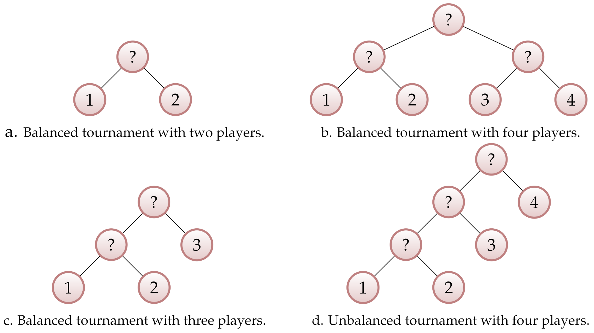
Example 1.

We consider examples of tournaments for sets of players with $1,2,3$ and 4 elements:

1. 

If $\Sigma =\left\{1\right\}$ then $\mathcal{T}(\Sigma )=\left\{1\right\}$.

2. 

If $\Sigma =\{1,2\}$ then $\mathcal{T}(\Sigma )=\left\{\right\{1,2\left\}\right\}$.

3. 

If $\Sigma =\{1,2,3\}$ then $\mathcal{T}(\Sigma )=\left\{\right\{\{1,2\},3\},\{\{1,3\},2\},\{\{3,2\},1\left\}\right\}$.

4. 

If $\Sigma =\{1,2,3,4\}$ then $\mathcal{T}(\Sigma )=\left\{\right\{\{1,2\},\{3,4\}\},\{\{1,3\},\{2,4\}\},\{\{1,4\},\{2,3\}\},\{\left\{\right\{1,2\},3\},4\},\dots \}$. It is not difficult to see that in this case there are 15 trees.

Some of the tournaments introduced in Example 1 are depicted graphically in Figure 1. Observe that the tournaments on the first row (labeled “a” and “b”) involve a number of elements that is a power of two ($2=2^1$ and $4=2^2$, respectively) and are fully balanced. However, the tournaments on the second row are not fully balanced, although the lower rightmost tournament involves $4=2^2$ players. However, intuitively, the tournament with three players (labeled “c”) should be accepted, as player 3 will enter the tournament only 1 round after players 1 and 2, i.e., it has a sense of “balancing”. However, the lower rightmost tournament with four players (labeled “d”) is not acceptable, as player 4 received an exemption from playing in the first two rounds, and this is considered unfair.

Figure 1. Tournaments of two and three players (first column) and four players (second column).

Proposition 1

(Counting tournaments). The set $\mathcal{T}(\Sigma )$ with $|\Sigma |=N$ players contains:

$$\frac{(2N-2)!}{(N-1)!\times 2^{N-1}}$$

(2)

elements.

Proof. 

The number of full binary tree structures with N leaves is equal to $C_{N-1}$ where $C_N$ is Catalan’s number [16] defined by:

$$C_N=\frac{1}{N+1}\left(\genfrac{}{}{0pt}{}{2N}{N}\right)$$

(3)

Now, each permutation of the N players can be attached to the leaves of a binary tree, thus obtaining $N!·C_{N-1}$ trees. However, the branches of each internal node can be exchanged, resulting in the same tree. There are $N-1$ internal nodes and therefore a total number of $2^{N-1}$ exchanges, resulting a number of trees given by:

$$\frac{N!·C_{N-1}}{2^{N-1}}=\frac{(2N-2)!}{(N-1)!·2^{N-1}}$$

(4)

q.e.d.    □

Example 2.

For example, if $N=3$ we obtain $\frac{4!}{2!\times 2^2}=3$ trees, while if $N=4$ we obtain $\frac{6!}{3!\times 2^3}=15$ trees. These results are consistent with Example 1.

A valid tournament should be balanced, i.e., each player should play (almost) the same number of games to win the tournament.

Analyzing the tournaments from Example 1 and Figure 1 we can observe that if $|\Sigma |\le 3$ then each element of $\mathcal{T}(\Sigma )$ represents a valid tournament. However, if $|\Sigma |=4$ then only 3 trees of $\mathcal{T}(\Sigma )$ represent valid tournaments. For example, $\left\{\right\{1,2\},\{3,4\left\}\right\}$ is a valid tournament as each player should play exactly two games to win the tournament. In this case we have a fully balanced tournament consisting of $N=2^2$ players. Moreover, $\left\{\right\{1,2\},3\}$ is also considered a valid tournament, as players 1 and 2 must play two games to win, while player 3 must play one game to win, i.e., has an exemption for the first round (the difference between the number of games played by each player is at most 1). However, $\left\{\right\{\{1,2\},3\},4\}$ is not a valid tournament, as players 1 and 2 must play three games to win the tournament, while player 4 must play a single match to win the tournament (the difference between the number of games played by each player is above 1, i.e., more than one exemption for a player is considered unfair).

Observe that a tree representing a valid tournament has the property that all its leaves are of height n or $n+1$ for a suitable value of n. Actually, the value of n can be determined from the given number of players N of the tournament and it represents the number of rounds of the tournament.

Let us consider a tournament with n rounds. It is not difficult to see that the maximum number of players is $N_{max}=2^n$ and it is obtained when in the first round we have a maximum number of $2^{n-1}$ games; therefore, for a tournament with n rounds we have:

$$2^{n-1}<N\le 2^n$$

(5)

Observe that from Equation (5) it follows that:

$$n=\lceil {log}_{2}N\rceil$$

(6)

Definition 2 (Balanced (valid) tournaments). Let $n\in \mathbb{N}$ be the number of rounds. Let Σ be a nonempty set of N players such that conditions (5) and (6) are fulfilled. Then the set ${\mathcal{T}}_n(\Sigma )$ of balanced trees with n layers representing the set of balanced (valid) tournaments with n rounds is defined as follows:

1. 

If $n=0$ then $N=1$ so we have a singleton set $\Sigma =\left\{i\right\}$. In this case ${\mathcal{T}}_0(\Sigma )=\left\{i\right\}$.

2. 

If $n\ge 1$, $t_1\in {\mathcal{T}}_{n-1}\left({\Sigma }_1\right)$, $t_2\in {\mathcal{T}}_{n-1}\left({\Sigma }_2\right)$, ${\Sigma }_1\cap {\Sigma }_2=\varnothing$ and ${\Sigma }_1\cup {\Sigma }_2=\Sigma$ then $t=\{t_1,t_2\}\in {\mathcal{T}}_n(\Sigma )$.

3. 

If $n\ge 2$, $t_1\in {\mathcal{T}}_{n-1}\left({\Sigma }_1\right)$, $t_2\in {\mathcal{T}}_{n-2}\left({\Sigma }_2\right)$ is a fully balanced tree (i.e., $|{\Sigma }_2|=2^{n-2}$), ${\Sigma }_1\cap {\Sigma }_2=\varnothing$ and ${\Sigma }_1\cup {\Sigma }_2=\Sigma$ then $t=\{t_1,t_2\}\in {\mathcal{T}}_n(\Sigma )$.

If $n\ge 1$ then there are $N\in 2^{n-1}+1\dots 2^n$ players. Then a tree $t\in {\mathcal{T}}_n(\Sigma )$ can be obtained either (i) by joining two balanced trees with $n-1$ layers or (ii) by joining one balanced tree with $n-1$ layers and one fully balanced tree with $n-2$ layers (all its leaves are on layer $n-2$), so in both cases the balancing condition of t is properly preserved.

Proposition 2

(Structure of a balanced tournament). Let $t\in {\mathcal{T}}_n(\Sigma )$ be a tournament of N players such that n is defined by Equation (6). Then the number of players starting in the first round is $\beta =2N-2^n$ and the number of players starting in the second round (waivers) is $\gamma =2^n-N$. Moreover, if $n\ge 1$ then the number of internal nodes of level 2 in the tree is equal to $\alpha =N-2^{n-1}$, i.e., $\beta =2\alpha$ and $\gamma =2^{n-1}-\alpha$.

Proof. 

First observe that if the number of players is a power of 2, i.e., $N=2^n$, then $\alpha =2^{n-1}=N/2$, $\beta =N$, and $\gamma =0$. This is trivially true, as in this case the tournament is fully balanced and all the players start in the first round (there are no exemptions).

The proof for the general case can be shown by induction on $n\in \mathbb{N}$.

For $n=0$ the tournament has $N=1$ players. In this case there is a single balanced tournament with $\gamma =0$ and $\beta =1$, so the property trivially holds.

For $n=1$ the tournament has $N=2$ players. In this case there is a single balanced tournament with $\alpha =1$, $\beta =2$ and $\gamma =0$, so the property trivially holds.

Let us now assume that the property holds for $k=0,1,\dots ,n$ and let us prove it for $k=n+1$. There are two cases.

Case 1. If $n\ge 1$, $t_1\in {\mathcal{T}}_n\left({\Sigma }_1\right)$, $t_2\in {\mathcal{T}}_n\left({\Sigma }_2\right)$, ${\Sigma }_1\cap {\Sigma }_2=\varnothing$ and ${\Sigma }_1\cup {\Sigma }_2=\Sigma$, let us consider $t=\{t_1,t_2\}\in {\mathcal{T}}_{n+1}(\Sigma )$ such that the second condition of Definition 2 is fulfilled. According to the induction hypothesis we have ${\gamma }_i=2^n-N_i$, ${\beta }_i=2N_i-2^n$, ${\alpha }_i=N_i-2^{n-1}$ for $i=1,2$ and $N=N_1+N_2$. Then $\gamma ={\gamma }_1+{\gamma }_2=2^{n+1}-(N_1+N_2)=2^{n+1}-N$. Similarly $\beta ={\beta }_1+{\beta }_2=2N-2^{n+1}$ and $\alpha ={\alpha }_1+{\alpha }_2=N-2^n$ q.e.d.

Case 2. If $n\ge 2$, $t_1\in {\mathcal{T}}_n\left({\Sigma }_1\right)$, $t_2\in {\mathcal{T}}_{n-1}\left({\Sigma }_2\right)$ is a fully balanced tree (i.e., $|{\Sigma }_2|=2^{n-1}$), ${\Sigma }_1\cap {\Sigma }_2=\varnothing$ and ${\Sigma }_1\cup {\Sigma }_2=\Sigma$, let us consider $t=\{t_1,t_2\}\in {\mathcal{T}}_{n+1}(\Sigma )$ such that the third condition of Definition 2 is fulfilled. According to the induction hypothesis we have ${\gamma }_1=2^n-N_1$, ${\beta }_1=2N_1-2^n$, ${\alpha }_1=N_1-2^{n-1}$, ${\gamma }_2=0$, ${\beta }_2=2^{n-1}$ and ${\alpha }_2=2^{n-2}$, $N_2=2(n-1)$, and $N=N_1+2^{n-1}$. Then $\beta ={\beta }_1=2(N_1+2^{n-1})-2^n-2^n=2N-2^{n+1}$. Similarly $\gamma ={\gamma }_1+{\beta }_2=2^n-N_1+2^{n-1}=2^n+2^{n-1}+2^{n-1}-N=2^{n+1}-N$ and similarly for $\alpha ={\alpha }_1=N_1-2^{n-1}=N-2^{n-1}-2^{n-1}=N-2^n$ q.e.d.

The relations $\beta =2\alpha$ and $\gamma =2^{n-1}-\alpha$ can be now easily checked.    □

Example 3

(Tournament structure design). Let us consider a tournament with $N=5$ players. In this case $n=3$, $\gamma =2^3-5=3$, $\alpha =2^2-3=1$, $\beta =2\times 5-2^3=2$. A tree representing a tournament with five players will have three layers such that the first layer consists of $\beta =2$ leaves (players) and the second layer consists of $2^{n-1}=2^2=4$ nodes among which there is $\alpha =1$ internal node and $\gamma =3$ leaves (players). One such a balanced tournament is depicted in Figure 2.

Figure 2. A balanced tournament of five players.

Proposition 3

(Counting balanced tournaments). The set ${\mathcal{T}}_n(\Sigma )$ with $|\Sigma |=N$ players contains:

$$\frac{N!·\left(\genfrac{}{}{0pt}{}{2^{n-1}}{\gamma }\right)}{2^{N-1}}$$

(7)

elements.

Proof. 

There are $\left(\genfrac{}{}{0pt}{}{2^{n-1}}{\gamma }\right)$ ways of choosing how the $\gamma$ players will enter second round. Their ordering matters so we multiply with $\gamma !$. Moreover those $\gamma$ players are arbitrarily chosen from the set of N players, so we multiply with $\left(\genfrac{}{}{0pt}{}{N}{\gamma }\right)$. Finally, the ordering of those $\beta$ remaining players that enter first round matters, so we also multiply with $\beta !$. For each internal node of the tree, exchanging its left and right sub-tree is a tournament invariant. There are $2^{N-1}$ independent ways of exchanging left and right sub-tree of the tree, so we must divide by $2^{N-1}$. We obtain:

$$\frac{\left(\genfrac{}{}{0pt}{}{N}{\gamma }\right)·\left(\genfrac{}{}{0pt}{}{2^{n-1}}{\gamma }\right)·\gamma !·\beta !}{2^{N-1}}=\frac{N!·\left(\genfrac{}{}{0pt}{}{2^{n-1}}{\gamma }\right)}{2^{N-1}}$$

(8)

A simpler proof is obtained by thinking about structures (i.e., “shapes”) of tournament trees. The selection of the “locations” of those $\gamma$ players entering second round can be achieved in $\left(\genfrac{}{}{0pt}{}{2^{n-1}}{\gamma }\right)$ ways. For each tree structure defined in this way there are $N!$ permutations of the leaves (players), thus defining a total number of $N!·\left(\genfrac{}{}{0pt}{}{2^{n-1}}{\gamma }\right)$ balanced tournament trees. Finally we divide by $2^{N-1}$ and we obtain Equation (7).    □

Example 4.

Let us check the number of balanced tournaments for several cases.

1. 

The number of balanced tournaments with $N=5$ players can be obtained as follows:

$$\frac{5!\times \left(\genfrac{}{}{0pt}{}{2^2}{3}\right)}{2^4}=30$$

(9)

It is not difficult to verify that this result is correct. In this case $\beta =2$. There are $\left(\genfrac{}{}{0pt}{}{5}{2}\right)=10$ ways of selecting those two players that will enter first round. We have one separate tournament by letting the winner of the game of these two players playing against each of the remaining three players in the second round. So in total there are $10\times 3=30$ balanced tournaments with five players.

2. 

For $n=3$ players we obtain:

$$\frac{3!\times \left(\genfrac{}{}{0pt}{}{2^1}{1}\right)}{2^2}=3$$

(10)

3. 

If $N=2^n$ then $\gamma =0$, thus we obtain our result for fully balanced tournaments from [1] stating that the total number of fully balanced tournaments is given by:

$$\frac{\left(2^n\right)!}{2^{2^n-1.}}$$

(11)

The number of fully balanced tournaments with two rounds is $\frac{\left(2^2\right)!}{2^{2^2-1}}=\frac{4!}{8}=3$. Observe that applying the formula, we obtain 315 fully balanced tournaments with three rounds. Let us obtain this result using a different reasoning. Let us count the number of a set with eight elements consisting of two subsets of four elements each. There are $\left(\genfrac{}{}{0pt}{}{8}{4}\right)/2=35$ possibilities, as we consider the four combinations of eight elements, and we divide by two as the order of the subsets of a partition does not matter; however, for each set of each partition there are three fully balanced tournaments of three rounds, so multiplying we obtain a total of nine possibilities. So the number of three-stage tournaments is $9\times 35=315$.

4. Optimal Tournaments

Each round of a tournament with n rounds defines possible games between players. Note that in a given tournament any two players can play in a game at one and only one of its rounds. This follows from the fact that for any two leaves of a binary tree there is a unique closest common ancestor. It follows that the tournament round $s_{i,j}$ where players $i,j$ can meet is a unique value in $1,2,\dots ,n$ and it is well defined. For example, referring to the tournament shown in Figure 2, $s_{2,4}=3$, $s_{1,5}=2$, and $s_{4,5}=1$.

Intuitively, the higher the quotations of players i and j, the better it is to let them meet in a higher stage of the tournament in order to increase the stakes of their games.

We assume in what follows that a quotation $q_i\in (0,+\infty )$ is available for each player $i\in \Sigma$. Quotations can be obtained from the players’ current ranking (as for example in international tennis tournaments ATP and WTA) or by other means.

Definition 3

(Tournament cost). Let $t\in {\mathcal{T}}_n(\Sigma )$ be a tournament with n rounds and let $s_{i,j}^t\in \{1,2,\dots ,n\}$ be the stage of t where players $i,j$ can meet. Let $q_i>0$ be the quotations of players for all $i\in \Sigma$. The cost of t is defined as:

$$Cost\left(t\right)=\sum _{i,j\in \Sigma ,i<j}{q}_i{q}_j{s}_{ij}^t$$

(12)

Definition 4

(Optimal tournament). A tournament such that its cost computed with Equation (12) is maximal is called an optimal tournament and it is defined by:

$$\begin{array}{cc}OptC(\Sigma )\hfill & =\underset{t\in {\mathcal{T}}_n(\Sigma )}{max}Cost\left(t\right)\hfill \\ t^{\ast }\hfill & ={argmax}_{t\in {\mathcal{T}}_n(\Sigma )}Cost\left(t\right)\hfill \end{array}$$

(13)

Obviously, better ranked players have a higher quotation. We assume that if player i has rank $r_i$ then its quota is $q_i$ such that whenever $r_i<r_j$ we have $q_i>q_j$. For example, if there are $N=2^n$ players then we can choose $q_i=N+1-r_i$ for all $i=1,\dots ,N$.

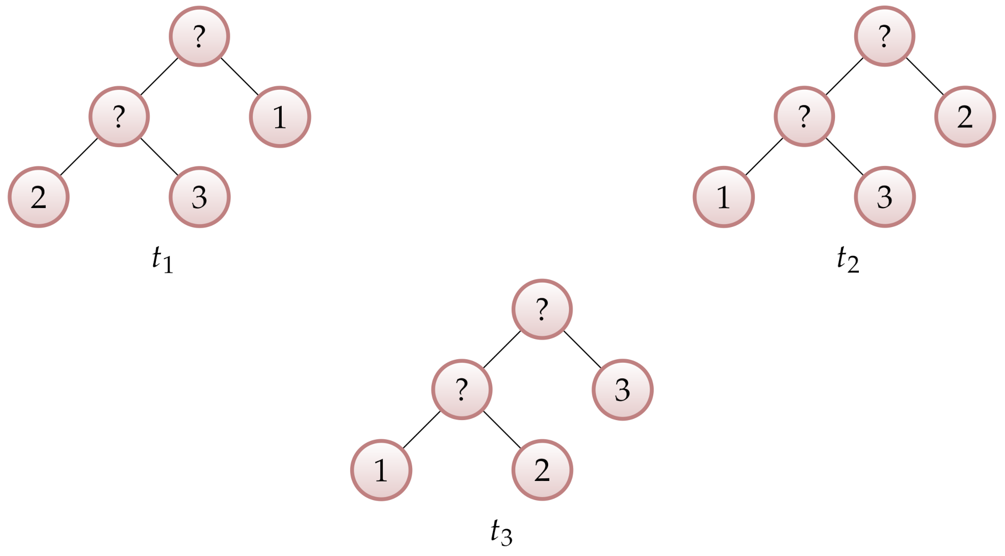
Example 5.

Let us consider the tournaments $t_1$, $t_2$, and $t_3$ with three players shown in Figure 3. Let us introduce:

$$\begin{array}{cc}A\hfill & =q_1{q}_2+q_1{q}_3+q_2{q}_3\hfill \\ S\hfill & =q_1+q_2+q_3\hfill \end{array}$$

(14)

Figure 3. Balanced tournaments with three players.

We obtain:

$$\begin{array}{cc}Cost\left(t_1\right)\hfill & =q_2{q}_{3}1+q_1{q}_{2}2+q_1{q}_{3}2=A+q_1(q_2+q_3)=A+q_1(S-q_1)\hfill \\ Cost\left(t_2\right)\hfill & =A+q_2(S-q_2)\hfill \\ Cost\left(t_3\right)\hfill & =A+q_3(S-q_3)\hfill \end{array}$$

(15)

The ordering of the costs depends on the ordering of the values of the function $q(S-q)$ for $q=q_1,q_2,q_3\in [0,S]$. This function is monotonically increasing on $[0,S/2]$ and monotonically decreasing on $[S/2,S]$. Observe that if $q_i\le S/2$, i.e., if neither player gets more than a half of the total quotation stake, then the ordering of the costs is given by the ordering of the quotations $q_i$.

Example 6.

Let us consider four players (see Table 1). We assume that each player has a unique rank from 1 to 4. Now, if we choose $q_i=5-r_i$ then, using this approach for defining players’ quota, player 2 with rank 4 is assigned quotation $q_2=1$. We consider the three tournaments $t_1,t_2,t_3\in T_2\left(\{1,2,3,4\}\right)$ from Figure 4. According to Equation (12), the cost of a tournament $t\in T_2\left(\{1,2,3,4\}\right)$ is:

$$\begin{array}{cc}\hfill Cost\left(t\right)& =\sum _{1\le i<j\le 4}^4{s}_{ij}^t{q}_i{q}_j\hfill \\ \hfill Cost\left(t\right)& =s_{12}^t·4\times 1+s_{13}^t·4\times 2+s_{14}^t·4\times 3+s_{23}^t·1\times 2+s_{24}^t·1\times 3+s_{34}^t·2\times 3\hfill \end{array}$$

(16)

Table 1. Players’ ranking and quotation for $n=4$.

Player i	Rank ${\mathit{r}}_{\mathit{i}}$	Quota ${\mathit{q}}_{\mathit{i}}=\mathit{n}+1-{\mathit{r}}_{\mathit{i}}$
1	1	4
4	2	3
3	3	2
2	4	1

Figure 4. Balanced tournaments with four players.

Substituting stage values $s_{ij}^t$ for each tournament from Table 2 into Equation (16) we obtain the tournaments’ cost values from Table 2. We observe that in this case the best tournament is $t_3$. Actually it can be easily checked that the best tournament is $t_3$ for whatever values of the quota that are decreasingly ordered according to the ranks.

Table 2. Games playing stages for each tournament of Figure 4 and their costs.

${\mathit{s}}^{{\mathit{t}}_1}$	1	2	3;	4	${\mathit{s}}^{{\mathit{t}}_2}$	1	2	3	4	${\mathit{s}}^{{\mathit{t}}_3}$	1	2	3	4
1		2	1	2	1		2	2	1	1		1	2	2
2			2	1	2			1	2	2			2	2
3				2	3				2	3				1
$Cost$	59					56					60
	Cost of $t_1$					Cost of $t_2$					Cost of $t_3$

5. Dynamic Programming Algorithm for Computing Optimal Tournaments

For any set of players $\Sigma$ we denote by $q_{\Sigma }$ the sum of quotations of the players in $\Sigma$.

$$\begin{array}{c}\hfill q_{\Sigma }=\sum _{i\in \Sigma }{q}_i\end{array}$$

(17)

Proposition 4

(Recurrence for tournament cost). Let $t\in {\mathcal{T}}_n(\Sigma )$ be an n-stage tournament such that Σ is a finite nonempty set with $N\in 2^{n-1}+1\dots 2^n$ elements. Then:

$$\begin{array}{c}\hfill Cost\left(t\right)=\left\{\begin{array}{cc}0\hfill & n=0\hfill \\ q_i·q_j\hfill & n=1,N=2,\Sigma =\{i,j\}\hfill \\ Cost\left(t_1\right)+Cost\left(t_2\right)+n{q}_{{\Sigma }_1}{q}_{{\Sigma }_2}\hfill & n\ge 2,t=\{t_1,t_2\},t_1\in \mathcal{T}\left({\Sigma }_1\right),\hfill \\ \hfill & t_2\in \mathcal{T}\left({\Sigma }_2\right),{\Sigma }_1\cup {\Sigma }_2=\Sigma ,{\Sigma }_1\cap {\Sigma }_2=\varnothing ,\hfill \\ \hfill & t_1\mathit{and}{t}_2\mathit{are}\mathit{balanced},\mathit{at}\mathit{most}\mathit{one}\mathit{has}n-2\hfill \\ \hfill & \mathit{levels}\mathit{and}\mathit{in}\mathit{this}\mathit{case}\mathit{it}\mathit{is}\mathit{fully}\mathit{balanced}\hfill \end{array}\right.\end{array}$$

(18)

Proof. 

If $n=0$ then $\Sigma$ has a single player so the result is obvious, as no games are played to determine the winner of the tournament.

If $n=1$ then $\Sigma$ has two players i and j so the result is obvious, as a single game is played to determine the winner of the tournament, between player i and player j.

If $n\ge 2$ then $t=\{t_1,t_2\}$. If $i\in {\Sigma }_1$ and $j\in {\Sigma }_2$ then $s_{ij}^t=n$. So Equation (12) gives:

$$\begin{array}{cc}\hfill Cost\left(t\right)=& \sum _{i,j\in {\Sigma }_1,i<j}{q}_i{q}_j{s}_{ij}^{t_1}+\sum _{i,j\in {\Sigma }_2,i<j}{q}_i{q}_j{s}_{ij}^{t_2}+\sum _{i\in {\Sigma }_1,j\in {\Sigma }_2}{q}_i{q}_j{s}_{ij}^t=\hfill \\ \hfill & Cost\left(t_1\right)+Cost\left(t_2\right)+n\sum _{i\in {\Sigma }_1,j\in {\Sigma }_2}{q}_i{q}_j=Cost\left(t_1\right)+Cost\left(t_2\right)+n{q}_{{\Sigma }_1}{q}_{{\Sigma }_2}\hfill \end{array}$$

(19)

The conditions from the Equation (18) follow directly from the recursive definition of balanced tournaments (Definition 2).    □

Proposition 5

(Recurrences for optimal tournaments).

1. 

The optimal tournament cost $OptC$ introduced by Equation (13) can be defined recursively as follows:

$$\begin{array}{c}\hfill OptC(\Sigma )=\left\{\begin{array}{cc}0\hfill & n=0,|\Sigma |=1\hfill \\ q_i·q_j\hfill & n=1,\Sigma =\{i,j\}\hfill \\ \underset{\begin{array}{c}{\Sigma }_1\cup {\Sigma }_2=\Sigma \\ {\Sigma }_1\cap {\Sigma }_2=\varnothing \end{array}}{max}OptC\left({\Sigma }_1\right)+OptC\left({\Sigma }_2\right)+n{q}_{{\Sigma }_1}{q}_{{\Sigma }_2}\hfill & n\ge 2,2^{n-1}<|\Sigma |\le 2^n\hfill \\ \hfill & 2^{n-2}\le \left|{\Sigma }_1\right|\le \hfill \\ \hfill & |{\Sigma }_2|\le 2^{n-1}\hfill \end{array}\right.\end{array}$$

(20)

2. 

The optimal tournament can be determined by recording the pairs of subsets $Opt(\Sigma )=({\Sigma }_1,{\Sigma }_2=\Sigma \setminus {\Sigma }_1)$ that maximize $OptC$ in Equation (20) for $n\ge 2$, $2^{n-1}<|\Sigma |\le 2^n$ as follows:

$$\begin{array}{c}\hfill OptS(\Sigma )=\underset{{\Sigma }_1,{\Sigma }_2\subseteq \Sigma }{argmax}OptC\left({\Sigma }_1\right)+OptC\left({\Sigma }_2\right)+n{q}_{{\Sigma }_1}{q}_{{\Sigma }_2}\end{array}$$

(21)

Note that the limits of argmax in Equation (21) must satisfy the conditions from the third branch of Equation (20). Note also that it is enough to record $Opt(\Sigma )={\Sigma }_1$ as ${\Sigma }_2=\Sigma \setminus {\Sigma }_1$.

Proof. 

The proof follows by applying the maximization operation in Equation (18) and observing that the term $n{q}_{{\Sigma }_1}{q}_{{\Sigma }_2}$ does not depend on $t=\{t_1,t_2\}$. The condition $|{\Sigma }_1|\le |{\Sigma }_2|$ ensures that a pair $\{{\Sigma }_1,{\Sigma }_2\}$ is uniquely considered (otherwise each pair will be considered twice as $\{{\Sigma }_1,{\Sigma }_2\}$ and $\{{\Sigma }_2,{\Sigma }_1\}$).

Moreover, the sets $OptS(\Sigma )$ can be used to construct an optimal tournament. Let ${\Sigma }^n=\Sigma$. We define: ${\Sigma }^{n-1}=OptS\left({\Sigma }^n\right)$, …, ${\Sigma }^0=OptS\left({\Sigma }^1\right)$. Then the optimal tournament $t^{\ast }$ can be defined recursively as follows:

$$\begin{array}{cc}\hfill t^{\ast }& =t^n\left({\Sigma }^n\right)\hfill \\ \hfill t^i\left({\Sigma }^i\right)& = \left\{\begin{array}{cc}\{t_1^{i-1}\left({\Sigma }^{i-1}\right),t_2^{i-1}({\Sigma }^i\setminus {\Sigma }^{i-1})\}\hfill & i\ge 1\hfill \\ j\hfill & i=0,{\Sigma }^0=\left\{j\right\}\hfill \end{array}\right.\hfill \end{array}$$

(22)

   □

Proposition 5 (Equation (20) in particular) can be used to design a dynamic programming algorithm for computing the optimal tournament and its cost. The dynamic programming algorithm can be implemented either with a bottom-up approach or using a top-down approach with memoization [17]. We will explore these possibilities in what follows by deriving a bottom-up dynamic programming algorithm for fully balanced tournaments as well as a top-down dynamic programming algorithm with memoization for the general case.

5.1. Top-Down Dynamic Programming Algorithm with Memoization

Proposition 6

(Top-down recursive application of Equation (20)). Let us assume that we want to compute $OptC(\Sigma )$ for $|\Sigma |=N$, $N\ge 2$, $2^{n-1}+1\le N\le 2^n$. According to Proposition 5, we must recursively explore all tournaments of shape $t=\{t_1,t_2\}$ such that $t_i\in T\left({\Sigma }_i\right)$, $|{\Sigma }_i|=N_i$, $i=1,2$, $N=N_1+N_2$. Then we should recursively apply Equation (20) only for the following values of $N_1$:

$$max\{N-2^{n-1},2^{n-2}\}\le N_1\le \lfloor N/2\rfloor$$

(23)

Proof. 

As $N=N_1+N_2$ and $N_1\le N_2$ we obtain:

$$N_1\le \lfloor N/2\rfloor$$

(24)

As $N=N_1+N_2$ and $2^{n-2}\le N_1\le 2^{n-1}$ we obtain:

$$\begin{array}{cc}\hfill 2^{n-2}& \le N_1\le 2^{n-1}\hfill \\ \hfill N-2^{n-1}& \le N_1\le N-2^{n-2}\hfill \end{array}$$

(25)

Combining (24) and (25) we obtain:

$$max\{N-2^{n-1},2^{n-2}\}\le N_1\le min\{2^{n-1},N-2^{n-2},\lfloor N/2\rfloor \}$$

(26)

It is not difficult to see that $\lfloor N/2\rfloor \le N/2\le 2^{n-1}$ and $\lfloor N/2\rfloor \le N/2<N-2^{n-2}$ so the value of right-hand side of Equation (26) is $\lfloor N/2\rfloor$, q.e.d.    □

Observe that for fully balanced tournaments $N=2^n$, so this top-down recursive process will generate subsets of sizes $2^{n-1},2^{n-2}\dots 2,1$.

Example 7.

Let us illustrate the application Equation (20) for $N=|\Sigma |=25$ players. The results are summarized in Table 3. It follows that solving the problem for a set of 25 players requires the solving of all subproblems corresponding to its subsets of $1,2,\dots ,16$ players; however, solving the problem for a set of 15 players requires the solving of all subproblems corresponding to its subsets of $1,2,3,4,7,8$ players. Moreover, solving the problem for a set of 14 players requires the solving of all subproblems corresponding to its subsets of $1,2,3,4,6,7,8$ players, while solving the problem for a set of 12 or 13 players requires the solving of all subproblems corresponding to its subsets of $1,2,3,4,5,6,7,8$ players.

Table 3. Games playing stages for each tournament and tournament costs.

|N|	$\mathit{n}=\lceil {log}_2\mathit{n}\rceil$	$\lfloor \frac{\mathit{N}}{2}\rfloor$	$\mathit{N}-2^{\mathit{n}-1}$	$2^{\mathit{n}-2}$	${\mathit{N}}_1^{\mathbf{min}},{\mathit{N}}_1^{\mathbf{max}}$	${\mathit{N}}_2^{\mathbf{min}},{\mathit{N}}_2^{\mathbf{max}}$
25	5	12	9	8	$9,12$	$13,16$
16	4	8	8	4	$8,8$	$8,8$
15	4	7	7	4	$7,7$	$8,8$
14	4	7	6	4	$6,7$	$7,8$
13	4	6	5	4	$5,6$	$7,8$
12	4	6	4	4	$4,6$	$6,8$
11	4	5	3	4	$4,5$	$6,7$
10	4	5	2	4	$4,5$	$5,6$
9	4	4	1	4	$4,4$	$5,5$
8	3	4	4	2	$4,4$	$4,4$
7	3	3	3	2	$3,3$	$4,4$
6	3	3	2	2	$2,3$	$3,4$
5	3	2	1	2	$2,3$	$2,3$
4	2	2	2	1	$2,2$	$2,2$
3	2	1	1	1	$1,1$	$2,2$
2	1	solved directly
1	0	solved directly

Proposition 6 sets the iteration bounds for exploring the subsets of players in the top-down approach. Combining the results of Propositions 5 and 6, we obtain the top-down approach for computing optimal balanced tournaments; see Algorithm 1.

Algorithm 1$OptTourCostTD(\Sigma ,N,q)$ top-down dynamic programming algorithm with memoization for computing the cost of the optimal tournament.

Global:$OptC$, initially ∅, maps subsets of players to costs of optimal tournaments.

$OptS$, initially ∅, maps subsets to sub-subsets for building optimal tournaments.

Input: $N\in {\mathbb{N}}^{\ast }$ represents the number of players.

q. Vector of size N representing the players’ quota.

$\Sigma$ such that $|\Sigma |=N$. $\Sigma$ represents the set of players.

Output: $C_{max}$. Cost of the optimal tournament for set $\Sigma$ of players.

$n\leftarrow \lceil {log}_{2}N\rceil$

if $n=0$ then

$C_{max}\leftarrow 0$

$S_{max}\leftarrow \varnothing$

else if $n=1$ (i.e., $\Sigma =\{i,j\}$) then

$C_{max}\leftarrow q_i\ast q_j$

$S_{max}\leftarrow \left\{i\right\}$

else

$P1\leftarrow 2^{n-2}$

$P2\leftarrow 2\ast P1$

$k_{max}\leftarrow \lfloor N/2\rfloor$

if $N\le P1+P2$ then

$k_{min}\leftarrow P1$

else

$k_{min}\leftarrow N-P2$

end if

$C_{max}\leftarrow -\infty$

for $k=k_{min},k_{max}$ do

for ${\Sigma }_1\subseteq \Sigma$ s.t. $|{\Sigma }_1|=k$ do

if ${\Sigma }_1\notin OptC$ then

$C_1\leftarrow OptTourCostTD({\Sigma }_1,k,q)$

else

$C_1\leftarrow OptC\left[{\Sigma }_1\right]$

end if

${\Sigma }_2\leftarrow \Sigma \setminus {\Sigma }_1$

if ${\Sigma }_2\notin OptC$ then

$C_2\leftarrow OptTourCostTD({\Sigma }_2,k,q)$

else

$C_2\leftarrow OptC\left[{\Sigma }_2\right]$

end if

$C\leftarrow C_1+C_2$

$ql\leftarrow 0$

for $i\in {\Sigma }_1$ do

$ql\leftarrow ql+q_i$

end for

$qr\leftarrow 0$

for $i\in {\Sigma }_2$ do

$qr\leftarrow qr+q_i$

end for

$C\leftarrow C+k\ast ql\ast qr$

if $C>Cmax$ then

$Cmax\leftarrow C$

$Smax\leftarrow {\Sigma }_1$

end if

end for

end for

end if

$OptC[\Sigma ]\leftarrow C_{max}$

$OptS[\Sigma ]\leftarrow S_{max}$

5.2. Bottom-Up Dynamic Programming Algorithm for Fully Balanced Tournaments

The cost of the optimal tournament is computed with the help of $OptC$ vector that is indexed by all the subsets of $\Sigma$ generated recursively by Equation (20), starting from the topmost set $\Sigma$. Note that for a fully balanced tournament we have $|\Sigma |=2^n$ and the process will generate exactly all the subsets of $\Sigma$ of cardinal: $2^0$, $2^1$, …$2^n$. Note that in this case the size of $OptC$ can be determined as:

$$S_n=\sum _{i=0}^{2^n}\left(\genfrac{}{}{0pt}{}{2^n}{2^i}\right)$$

(27)

Additionally we must save in vector $OptS$ of size $S_n$ the subsets ${\Sigma }^{\prime }$ determined using Equation (21), such that we can reuse them to construct the optimal tournament using Equation (22). Our proposed algorithm is presented as Algorithm 2.

Algorithm 2$OptTourCostBU(\Sigma ,N=2^n,q)$ bottom up dynamic programming algorithm for computing the cost of optimal fully balanced tournaments.

Input: $N=2^n,n\in \mathbb{N}$. N represents the number of players.

q. Vector of size N representing the players’ quota.

$\Sigma$ such that $|\Sigma |=2^n$. $\Sigma$ represents the set of players.

Output: $OptC$. Vector of costs of the optimal sub-tournaments.

$OptS$. Vector of sets to construct the optimal tournament.

1: for $i=1,N$ do

2:      $OptC\left[\right\{i\left\}\right]\leftarrow 0$

3: end for

4: for $k=1,n$ do

5:        for ${\Sigma }_1\subseteq \Sigma$ s.t. $|{\Sigma }_1|=2^k$ do

6:           $Cmax\leftarrow -\infty$

7:           for ${\Sigma }^{\prime }\subseteq {\Sigma }_1$ s.t. $|{\Sigma }^{\prime }|=2^{k-1}$ do

8:              $C\leftarrow OptC\left({\Sigma }^{\prime }\right)+OptC({\Sigma }_1\setminus {\Sigma }^{\prime })$

9:              $ql\leftarrow 0$

10:              for $i\in {\Sigma }^{\prime }$ do

11:                $ql\leftarrow ql+q_i$

12:              end for

13:              $qr\leftarrow 0$

14:              for $i\in {\Sigma }_1\setminus {\Sigma }^{\prime }$ do

15:                 $qr\leftarrow qr+q_i$

16:              end for

17:              $C\leftarrow C+k\ast ql\ast qr$

18:              if $C>Cmax$ then

19:                 $Cmax\leftarrow C$

20:                 $Smax\leftarrow {\Sigma }^{\prime }$

21:              end if

22:           end for

23:           $OptC\left[{\Sigma }_1\right]\leftarrow Cmax$

24:           $OptS\left[{\Sigma }_1\right]\leftarrow Smax$

25:          end for

26: end for

5.3. Computing an Optimal Tournament

Note that both Algorithms 1 and 2 determine the $OptS$ structure that records the split points for each subset of players according to Equation (20). The $OptS$ structure can be used to actually build an optimal tournament according to Algorithm 3 using Equation (22).

Algorithm 3:$OptTour(\Sigma ,N,OptS)$ algorithm for computing the optimal tournament.

Input:$\Sigma$ representing the set of players.

$N\in {\mathbb{N}}^{\ast }$ representing the number of players.

$OptS$. Structure determined either by Algorithm 1 or by Algorithm 2.

Output: Returns the optimal tournament.

1: if $N=1$ (i.e., $\Sigma =\left\{j\right\}$) then

2:   return j

3: end if

4: ${\Sigma }_1\leftarrow OptS(\Sigma )$

5: $N_1\leftarrow \left|{\Sigma }_1\right|$

6: ${\Sigma }_2\leftarrow \Sigma \setminus {\Sigma }_1$

7: $t_1\leftarrow OptTour({\Sigma }_1,N_1,OptS)$

8: $t_2\leftarrow OptTour({\Sigma }_2,N-N_1,OptS)$

9: return$\{t_1,t_2\}$

5.4. Correctness and Complexity Results

Proposition 7

(Correctness of Algorithms 1–3).

a. 

The value $C_{max}=OptC[\Sigma ]$ computed by Algorithms 1 and 2 represents the cost of the optimal tournament in both cases.

b. 

The tournament determined by Algorithm 3 is the optimal tournament.

Proof. 

Proof of a. Algorithms 1 and 2 compute the values of $OptC$ and $OptS$ either in top-down or bottom-up fashion for all the subsets that are required to determine the optimal tournament for the set $\Sigma$ of players. The computation follows Equations (20) and (21); therefore the correctness of this point follows from Propositions 5 and 6.

Proof of b. Algorithm 3 computes the optimal tournament using Equations (22). As values of $OptS$ are correctly determined according to point “a”, it follows that the tournament computed by Algorithm 3 is the optimal tournament.    □

Proposition 8

(Complexity of Algorithms 2 and 3). Let us consider tournaments with N players.

a. 

Space complexity of Algorithm 2 is $\Theta \left(\frac{2^N}{\sqrt{N}}\right)$.

b. 

Time complexity of Algorithm 2 is $\Theta \left({\left(2\sqrt{2}\right)}^N\right)$.

c. 

Space complexity of Algorithm 1 is $\Theta \left(\frac{2^N}{\sqrt{N}}\right)$ for fully balanced tournaments and $O\left(2^N\right)$ in the general case.

d. 

Time complexity of Algorithm 1 is $O(3^N·N\sqrt{N})$.

e. 

Time complexity of Algorithm 3 is $\Theta \left(N\right)$.

Proof. 

The proof is using the Stirling approximation of the factorial, written in inequality form ([18]), in fact showing that $p!=\Theta \left(\sqrt{p}{\left(\frac{p}{e}\right)}^p\right)$:

$$\sqrt{2\pi }\le \frac{p!}{\sqrt{p}{\left(\frac{p}{e}\right)}^p}\le e$$

(28)

Using this observation it is not difficult to prove that:

$$\left(\genfrac{}{}{0pt}{}{2p}{p}\right)=\Theta \left(\frac{2^{2p}}{\sqrt{p}}\right)$$

(29)

Proof of a. The space complexity of Algorithms 2 and 3 is given by the size of structures $OptC$ and $OptS$ (see Equation (27)); however, the asymptotically dominant term of this summation is $\left(\genfrac{}{}{0pt}{}{2^n}{2^{n-1}}\right)$. Then the result follows using Equation (29) for $p=2^{n-1}$.

Proof of b. Algorithm 2 contains one “for” loop (lines 4–26) including other three nested “for” loops. The first inner “for” loop (lines 5–25) is executed $\left(\genfrac{}{}{0pt}{}{N}{2^k}\right)$ times. The second inner “for” loop (lines 7–22) is executed $\left(\genfrac{}{}{0pt}{}{2^k}{2^{k-1}}\right)$ times. The third inner “for” loop (lines 10–12 and 14–16) is executed $2^{k-1}$ times. The total number of steps of Algorithm 2 is given by:

$$\sum _{k=1}^n\left(\genfrac{}{}{0pt}{}{N}{2^k}\right)\left(\genfrac{}{}{0pt}{}{2^k}{2^{k-1}}\right)2^{k-1}$$

(30)

Observe that the asymptotically dominant term of this summation is obtained for $k=n-1$ and it can be transformed using Equation (29), thus concluding the proof:

$$\left(\genfrac{}{}{0pt}{}{N}{2^{n-1}}\right)\left(\genfrac{}{}{0pt}{}{2^{n-1}}{2^{n-2}}\right)2^{n-2}=\Theta \left(\frac{2^{2^n}}{\sqrt{2^{n-1}}}\frac{2^{2^{n-1}}}{\sqrt{2^{n-2}}}{2}^{n-2}\right)=\Theta \left(\frac{1}{\sqrt{2}}{2}^N{2}^{N/2}\right)=\Theta \left({\left(2\sqrt{2}\right)}^N\right)$$

(31)

Proof of c. If N is a power of two, i.e., we have a fully balanced tournament, the memory consumption is exactly as in case a, so the first result follows trivially. Otherwise, the space consumption of tables $OptC$ and $OptS$ has an upper bound given by the size of the power set of $\Sigma$, and the result follows immediately.

Proof of d. Let us first observe that in order to determine the cost of an optimal tournament with N players we need to know the costs of optimal tournaments for $N_1$ and $N_2$ players such that $N=N_1+N_2$ and condition of Equation (23) holds. It is not difficult to observe that:

$$\frac{N}{4}<N_1\le N_2<\frac{3N}{4}$$

(32)

First note that the upper bound of $N_2$ follows from the lower bound of $N_1$, so it is enough to show the lower bound of $N_1$. Let us assume by contradiction that:

$$\frac{N}{4}\ge max\{N-2^{n-1},2^{n-2}\}$$

(33)

It follows that:

$$\frac{N}{2}=\frac{N}{4}+\frac{N}{4}\ge N-2^{n-1}+2^{n-2}=N-2^{n-2}$$

(34)

so:

$$N\le 2^{n-1}$$

(35)

and thus contradicting (5).

It is easier to analyze the complexity of Algorithm 1 by thinking “bottom-up” rather than “top-down”. The complexity will be the same, as the role of the memorization technique is just to evaluate exactly once the cost of a tournament for each subset of players. So we must determine the cost for a subset of $i=\frac{N}{4},\frac{N}{4}+1,\dots ,\frac{3N}{4}$ players ($\lfloor ·\rfloor$ can be omitted without losing generality); therefore the total running time has the following upper bound:

$$\sum _{p=\frac{N}{4}}^{p=\frac{3N}{4}}\left(\genfrac{}{}{0pt}{}{N}{p}\right)\sum _{k=\frac{p}{4}}^{\frac{3p}{4}}\left(\genfrac{}{}{0pt}{}{p}{k}\right)k$$

(36)

Although $\left(\genfrac{}{}{0pt}{}{p}{k}\right)=\left(\genfrac{}{}{0pt}{}{p}{p-k}\right)$, so grouping terms with complementary binomial coefficients of inner sum of (36), noticing that $\left(\genfrac{}{}{0pt}{}{p}{k}\right)\le \left(\genfrac{}{}{0pt}{}{p}{\frac{p}{2}}\right)$ and using (29), the inner sum has an upper bound of:

$$p·\sum _{k=\frac{p}{4}}^{\frac{p}{2}}\left(\genfrac{}{}{0pt}{}{p}{k}\right)\le p·\frac{p}{4}·\Theta \left(\frac{2^p}{\sqrt{p}}\right)\le N\sqrt{N}·\Theta \left(2^p\right)$$

(37)

Now, substituting (37) in (36) we obtain the following upper bound of the running time:

$$N\sqrt{N}·\sum _{p=\frac{N}{4}}^{p=\frac{3N}{4}}\left(\genfrac{}{}{0pt}{}{N}{p}\right)·\Theta \left(2^p\right)\le N\sqrt{N}·\sum _{p=0}^{p=N}\left(\genfrac{}{}{0pt}{}{N}{p}\right)·\Theta \left(2^p\right)=\Theta (3^N·N\sqrt{N})$$

(38)

As this is in fact only an upper bound of our running time, the result of point e follows (i.e., with O rather than $\Theta$).

Proof of e. Observe that the time complexity of Algorithm 3 satisfies the recursive equation $T\left(\right|\Sigma \left|\right)=T\left(\right|{\Sigma }_1\left|\right)+T\left(\right|{\Sigma }_2\left|\right)$. Unfolding this equation with the substitution method yields an asymptotic execution time $\Theta \left(\right|\Sigma \left|\right)=\Theta \left(N\right)$.    □

5.5. Sub-Optimal Algorithms

The dynamic programming approach for construing optimal tournaments has the disadvantage that the full exploration of the search space becomes prohibitive for larger tournaments. Our experiments (see Section 6) clearly show that this approach is unfeasible for tournaments of more than $n=16$ players; however, the dynamic programming algorithms can be easily adapted to explore a smaller size of the search space, leading to sub-optimal solutions. The exploration strategy can be used to tune the trade-off between the complexity of the computation and the “gap” between the provided sub-optimal solution and the actual optimal solution.

The resulting sub-optimal algorithms follow a strictly top-down approach that can be the best described as divide-and-conquer. At each decision point, rather than exploring all pairs of subsets $({\Sigma }_1,{\Sigma }_2)$ satisfying conditions of Equation (20), only few such pairs (ideally only 1) are selected for exploration. This selection strategy can be deterministic, based on heuristic principles, or stochastic based on stochastic sampling subsets of $\Sigma$ satisfying the conditions of Equation (20). The strictly top-down approach has the advantage that it avoids the use of temporary structures $OptS$ and $OptC$ and of the additional algorithm $OptTour$ to build the solution. Rather, the top-down approach will build the solution directly, using the recursive divide-and-conquer approach.

The general approach of a sub-optimal algorithm following a top-down divide and conquer approach is presented as Algorithm 4. Note that this algorithm is using a specific strategy to explore only a few subsets of $\Sigma$ defined by $Strategy(\Sigma ,k_{min},k_{max})\subseteq 2^{\Sigma }$ and satisfying the conditions of Equation (20).

Proposition 9

(Complexity of Algorithm 4). Let us consider tournaments for N players and let n be the number of stages of a balanced tournament. Then the time complexity of Algorithm 4 is $O\left(N^{1+{log}_{2}s}\right)$ where s is the average number of subsets of Σ explored by the strategy of the algorithm.

Proof. 

It is not difficult to observe that the time complexity of Algorithm 4 satisfies the following recurrence:

$$T\left(\right|\Sigma \left|\right)=s·\left(T\right(|{\Sigma }_1\left|\right)+T\left(\right|\Sigma \setminus {\Sigma }_1\left|\right))$$

(39)

Applying the substitution method for Equation (39) we obtain:

$$T\left(\right|\Sigma \left|\right)=\sum _{i\in \Sigma }{s}^{h_i}·O\left(1\right)$$

(40)

For each $i\in \Sigma$, $h_i$ from Equation (40) denotes the height of leaf i in the tournament tree, so $h_i\le n\le {log}_{2}N$. So:

$$T\left(\right|\Sigma \left|\right)=N·O\left(s^{lo{g}_{2}N}\right)=O\left(N^{1+{log}_{2}s}\right)$$

(41)

q.e.d.    □

Algorithm 4$OptTourCostSubOpt(\Sigma ,N,q,S)$ top-down divide-and-conquer algorithm for computing a sub-optimal tournament.

Input:$N\in {\mathbb{N}}^{\ast }$ represents the number of players.

q. Vector of size N representing the players’ quota.

$\Sigma$ such that $|\Sigma |=N$. $\Sigma$ represents the set of players.

$S={\sum }_{i\in \Sigma }{q}_i$. Sum of players’ quotations.

Output:$C_{max}$. Cost of the sub-optimal tournament for set $\Sigma$ of players.

$t_{max}$. Sub-optimal tournament tree.

1: $n\leftarrow \lceil {log}_{2}N\rceil$

2: if $n=0$ (i.e., $\Sigma =\left\{i\right\}$) then

3:    $C_{max}\leftarrow 0$

4:    $t_{max}\leftarrow i$

5: else if $n=1$ (i.e., $\Sigma =\{i,j\}$) then

6:    $C_{max}\leftarrow q_i\ast q_j$

7:    $t_{max}\leftarrow \{i,j\}$

8: else

9:    $P1\leftarrow 2^{n-2}$

10:    $P2\leftarrow 2\ast P1$

11:    $k_{max}\leftarrow \lfloor N/2\rfloor$

12:    if $N\le P1+P2$ then

13:      $k_{min}\leftarrow P1$

14:    else

15:      $k_{min}\leftarrow N-P2$

16:    end if

17:    $C_{max}\leftarrow -\infty$

18:    for ${\Sigma }_1\in Strategy(\Sigma ,k_{min},k_{max})$ do

19:      $S_1\leftarrow 0$

20:      for $i\in {\Sigma }_1$ do

21:        $S_1\leftarrow S_1+q_i$

22:      end for

23:      $k\leftarrow |{\Sigma }_1|$

24:      $(C_1,t_1)\leftarrow OptTourCostSubOpt({\Sigma }_1,k,q,S_1)$

25:      $(C_2,t_2)\leftarrow OptTourCostSubOpt(\Sigma \setminus {\Sigma }_1,N-k,q,S-S_1)$

26:      $C\leftarrow C_1+C_2+k\ast S_1\ast (S-S_1)$

27:      if $C>C_{max}$ then

28:        $C_{max}\leftarrow C$

29:        $t_{max}\leftarrow (t_1,t_2)$

30:      end if

31:     end for

32: end if

33: return$(C_{max},t_{max})$

Observe that if $s=1$ then the time complexity of Algorithm 4 is linear in the number N of players. Moreover, if $s>1$ then the time complexity of the algorithm is polynomial in N and the degree of the polynomial grows logarithmically with s.

5.5.1. Deterministic Sub-Optimal Algorithms

We define a deterministic sub-optimal algorithm by letting ${\Sigma }_1$ consist of the smallest set of players $1,2,\dots ,k$ such that $k\ge k_{min}$ and $q_{{\Sigma }_1}>q_{\Sigma }/2$.

The rationale of this choice is to try to make the product $q_{{\Sigma }_1}{q}_{{\Sigma }_2}$ from Equation (20) as high as possible. As $q_{{\Sigma }_1}+q_{{\Sigma }_2}=q_{\Sigma }$ is constant, we try to make the values $q_{{\Sigma }_1}$ and $q_{{\Sigma }_2}$ as close as possible, while maintaining the constraints on the size of subset ${\Sigma }_1$.

We can define three variants of the deterministic sub-optimal algorithm by considering the sequence of players’ quotations to be: (i) unchanged, i.e., as it was provided as input; (ii) increasingly sorted; (iii) decreasingly sorted.

5.5.2. Stochastic Sub-Optimal Algorithms

We define a stochastic sub-optimal algorithm by letting ${\Sigma }_1$ consist of a family of randomly chosen subsets of players of ${\Sigma }_1\subseteq \Sigma$ such that $k_{max}\ge \left|{\Sigma }_1\right|\ge k_{min}$. This is easily achieved by randomly choosing the number of players k uniformly distributed in $[k_{min},k_{max}]$ and then randomly choosing a subset ${\Sigma }_1$ of k elements and uniformly distributed in $\Sigma$.

The number of chosen subsets ${\Sigma }_1$ explored by the algorithm is a parameter denoted by $N_{sample}$ and it usually has a low number, as it directly influences the complexity of the algorithm according to Proposition 9, $s=N_{sample}$. For example, if $N_{sample}=1$ the complexity of the algorithm is $O\left(N\right)$, if $N_{sample}=2$ the complexity of the algorithm is $O\left(N^2\right)$ and if $N_{sample}=4$ the complexity of the algorithm is $O\left(N^3\right)$.

6. Implementation and Experiments

6.1. Implementation Issues

There were several issues that we had to address by our experimental implementation of Algorithms 1–3.

Firstly, we have chosen to represent sets as arrays of bits, as well as using the integer value that is equivalent to the binary representation as an array of bits.

Secondly, for generating subsets of given size (i.e., combinations) we have used Algorithm 7.2.1.2L from [19] for generating permutations with repetitions of binary arrays. Basically the subsets representing combinations of k elements of a set with $n\ge k$ elements are all the permutations with repetitions of a binary vector of n elements containing exactly k elements equal to 1.

Thirdly, we had to choose an efficient representation of $OptC$ and $OptS$ structures. Their operation is crucial for the efficient implementation of some of our algorithms. As for our implementation we have chosen Python platform, we decided to implement $OptC$ and $OptS$ using subset-indexed dictionaries that map subsets of $\Sigma$ to costs and to subsets necessary for building optimal tournaments, respectively. The subsets representing the dictionary keys are defined as integer values of their characteristic vector in binary format. As Python dictionaries are efficiently implemented using hash tables, an average $O\left(1\right)$ time complexity is expected for lookup operations.

Finally, for the implementation of the random selection of subsets we have used the array of bits representation of sets and we have applied the random.permute function from NumPy package to return a randomly permuted array representing a random subset.

6.2. Experimental Results

Our experiments were developed in Python 3.7.3 using Jupyter Notebook on an x64-based PC with a 2 cores/4 threads Intel© Core™i7-5500U CPU at 2.40 GHz running Windows 10 (The experimental code is available at http://software.ucv.ro/~cbadica/tour.zip accessed on 2 September 2021).

According to our findings, there are no algorithms directly available to be compared with our own proposals. There are two main causes for this. First, we consider an integrated approach of tournament design, rather than a process involving two separated stages for structure design and seeding. Secondly, we do not use probabilistic information in our cost function, thus hindering the direct comparison of tournament cost values.

We took a different path for evaluating our proposals. We have implemented optimal algorithms, as well as several versions of sub-optimal algorithms and then compared their outcomes in terms of running time and optimality. So finally we have implemented and experimentally evaluated eight algorithms, as presented in Table 4.

Table 4. Table presenting the list of implemented optimal and sub-optimal algorithms for balanced tournaments.

Algorithm	Description	Optimality	Players’ Number
$OptTD$	Dynamic programming top-down with memoization approach—Algorithm 1	Optimal	Arbitrary natural number
$OptBU$	Dynamic programming bottom-up approach—Algorithm 2	Optimal	Exact power of 2
$SubOpt{D}_1$	Deterministic sub-optimal approach—Algorithm 4 with deterministic strategy and unchanged quotation sequence	Sub-optimal	Arbitrary natural number
$SubOpt{D}_2$	Deterministic sub-optimal approach—Algorithm 4 with deterministic strategy and increasingly sorted quotation sequence	Sub-optimal	Arbitrary natural number
$SubOpt{D}_3$	Deterministic sub-optimal approach—Algorithm 4 with deterministic strategy and decreasingly sorted quotation sequence	Sub-optimal	Arbitrary natural number
$SubOpt{S}_1$	Stochastic sub-optimal approach—Algorithm 4 with stochastic strategy and $N_{sample}=1$	Sub-optimal	Arbitrary natural number
$SubOpt{S}_2$	Stochastic sub-optimal approach—Algorithm 4 with stochastic strategy and $N_{sample}=2$	Sub-optimal	Arbitrary natural number
$SubOpt{S}_3$	Stochastic sub-optimal approach Algorithm 4 with stochastic strategy and $N_{sample}=3$	Sub-optimal	Arbitrary natural number

Note that for the optimal algorithms there are at least two restrictions that hinder a complete experimental comparison with the rest of the algorithms. Firstly, their high computational complexity limits their applicability only to small number of players. Secondly, the dynamic programming bottom-up algorithm works only for a number of players that is an exact power of 2. We have only checked it for $N=4,8,16$.

Our data set includes multiple sequences of players’ quotations. For each $N=3,4,\dots 50$ we generated a sequence of quotations $q_1,q_2,\dots ,q_N$ with integer values $q_i$ randomly chosen with a uniform distribution in the interval $[q_{min}=1,q_{max}=9]$. This data set was used to experimentally evaluate the algorithms from Table 4, as follows:

• All the sequences of the data set were used for testing algorithms $SubOpt{D}_i$ and $SubOpt{S}_i$ for $i=1,2,3$.
• The optimal algorithm $OptTD$ was evaluated only for sequences corresponding to $N=3,\dots ,16$ players. The reason is that the algorithm has a too high computational complexity and we limited the running time of each problem instance to 5 min.
• The optimal algorithm $OptBU$ was evaluated only for sequences corresponding to $N=4,8,16$ players. The reason is both the high computational complexity of the algorithm and the fact that this algorithm was designed to work only with a number of players that is an exact power of 2.

For each algorithm, we recorded the (sub-)optimal cost of the output tournament, as well as the running time. Stochastic algorithms $SubOpt{S}_i$ for $i=1,2,3$ were evaluated by repeating their execution 10 times for each input sequence of quotations from the data set and recording the minimum, maximum, and average costs, as well as the average running times.

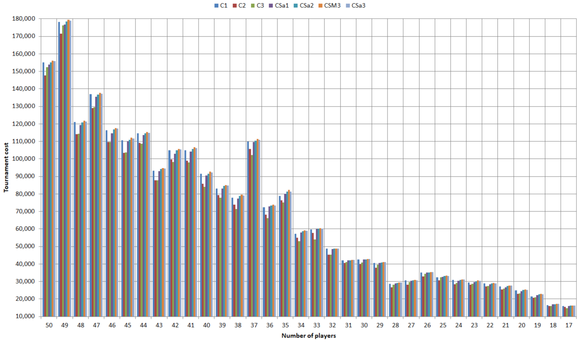
Figure 5 presents the sub-optimal costs produced by $SubOpt{D}_i$ and $SubOpt{S}_i$ algorithms for $i=1,2,3$. The figure plots costs $C_i$ produced by algorithms $SubOpt{D}_i$ for $i=1,2,3$, as well as average costs $CS{a}_i$ produced by algorithms $SubOpt{S}_i$ for $i=1,2,3$ and the maximum cost $CS{M}_3$ produced by the 10-times repeated execution of algorithm $SubOpt{S}_3$. Note that we included maximum cost only for this case, as it should be obvious that it is expected that stochastic algorithm $SubOpt{S}_3$ will produce the best results among $SubOpt{S}_i$ for $i=1,2,3$ because it uses the highest number of samplings $N_{sample}=3$.

Figure 5. Sub-optimal tournament costs determined by sub-optimal algorithms on different quotations’ sequences for various number of players.

Analyzing Figure 5, we first observe that the relative difference of the costs produced by the various algorithms on the same input sequence is rather low. This is expected, as quotations $q_i$ were generated as integer values from a small interval $1\le q_i\le 9$ while the cost tends to reach significantly higher values. For example, analyzing in detail the results obtained for the sample with $N=50$ players we observe that the relative difference between the smallest and the highest cost obtained (147,555 and 156,203) is of only $5.53\%$. We can also notice that the best results among sub-optimal algorithms were obtained by algorithm $SubOpt{S}_3$, while the worst results were obtained by algorithms $SubOpt{D}_2$ and $SubOpt{D}_3$. It might look a bit surprising that algorithm $SubOpt{D}_1$ appears to be superior to $SubOpt{D}_2$ and $SubOpt{D}_3$; however, taking into account how the data set was generated, this could be explained by the fact that algorithm $SubOpt{D}_1$ is actually using a random permutation of the quotations’ sequence that provides a better balance of the total quotation distribution between the two subsets ${\Sigma }_1$ and $\Sigma \setminus {\Sigma }_1$ (see Algorithm 4) than algorithms $SubOpt{D}_2$ and $SubOpt{D}_3$. One final remark, also observed experimentally, is that algorithms $SubOpt{D}_2$ and $SubOpt{D}_3$ produce the same sub-optimal costs if the number of players is an exact power of 2 (i.e., 16 and 32 on Figure 5). This is an immediate consequence on the logic behind their strategy definition.

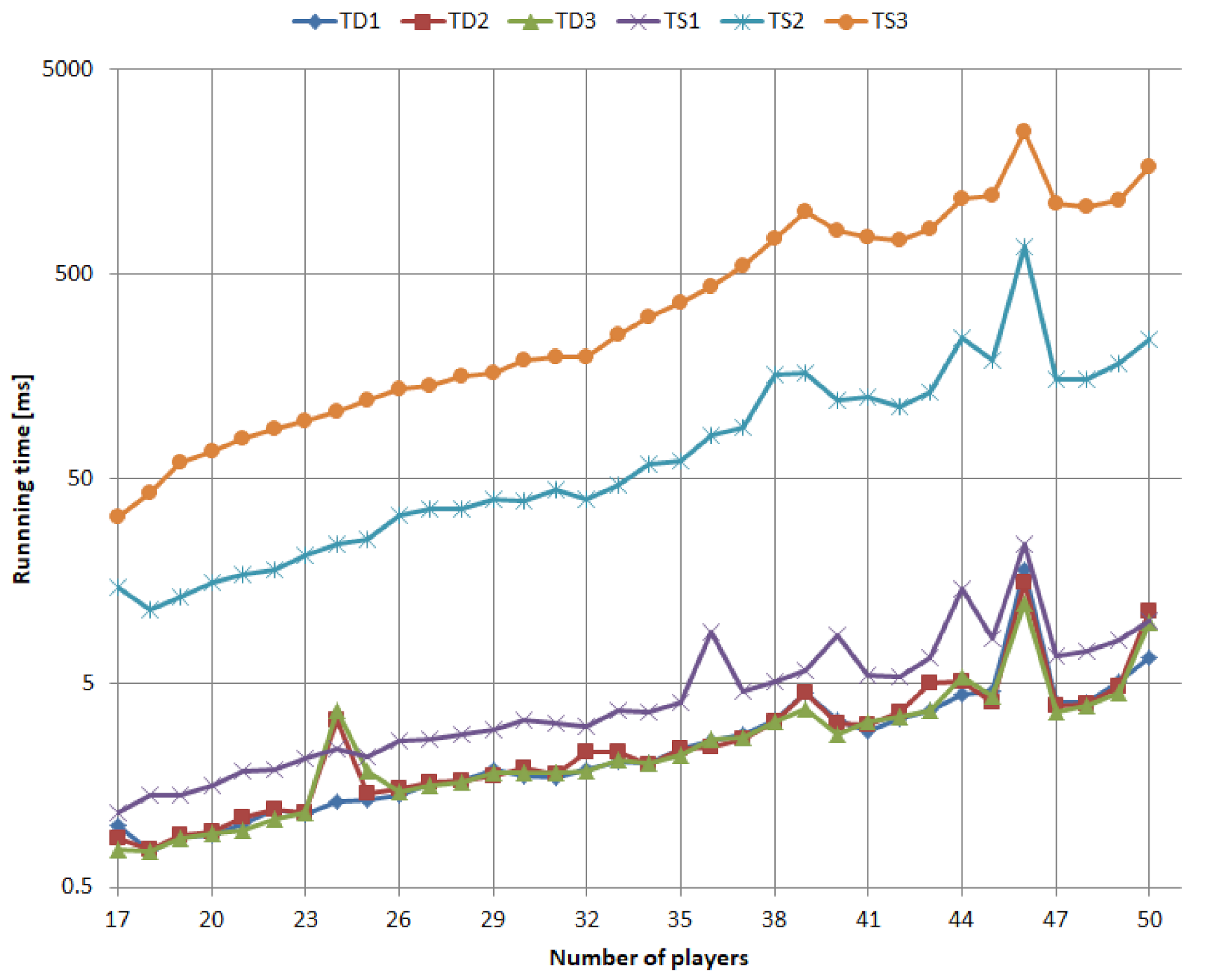
Figure 6 presents the running times $T{D}_i$ and $T{S}_i$ of algorithms $SubOpt{D}_i$ and $SubOpt{S}_i$ for $i=1,2,3$. The time figures are given in milliseconds and presented on a logarithmic scale and they were computed by taking the average for 10 executions of the algorithm on the same input data. First observe that deterministic versions $SubOpt{D}_i$ are the fastest and they have virtually almost the same running times. This can be easily explained by the low computational complexity of the implementation of their underlying strategies. Basically, their strategies use the same mechanism, while the additional sorting of the sequence of quotations adds a negligible cost as it is performed before the actual core processing of the algorithms. Second, the highest execution time is achieved, as expected, by $SubOpt{S}_3$. This algorithm has the highest computational complexity among sub-optimal algorithms, as it is using three subset samples during the top-down search. From Figure 6 it also follows that the highest average execution time was obtained for the sequence of quotations with $N=46$ players and its value was $2.49$ s.

Figure 6. Running times on logarithmic scale of sub-optimal algorithms on different quotations’ sequences for a variable number of players.

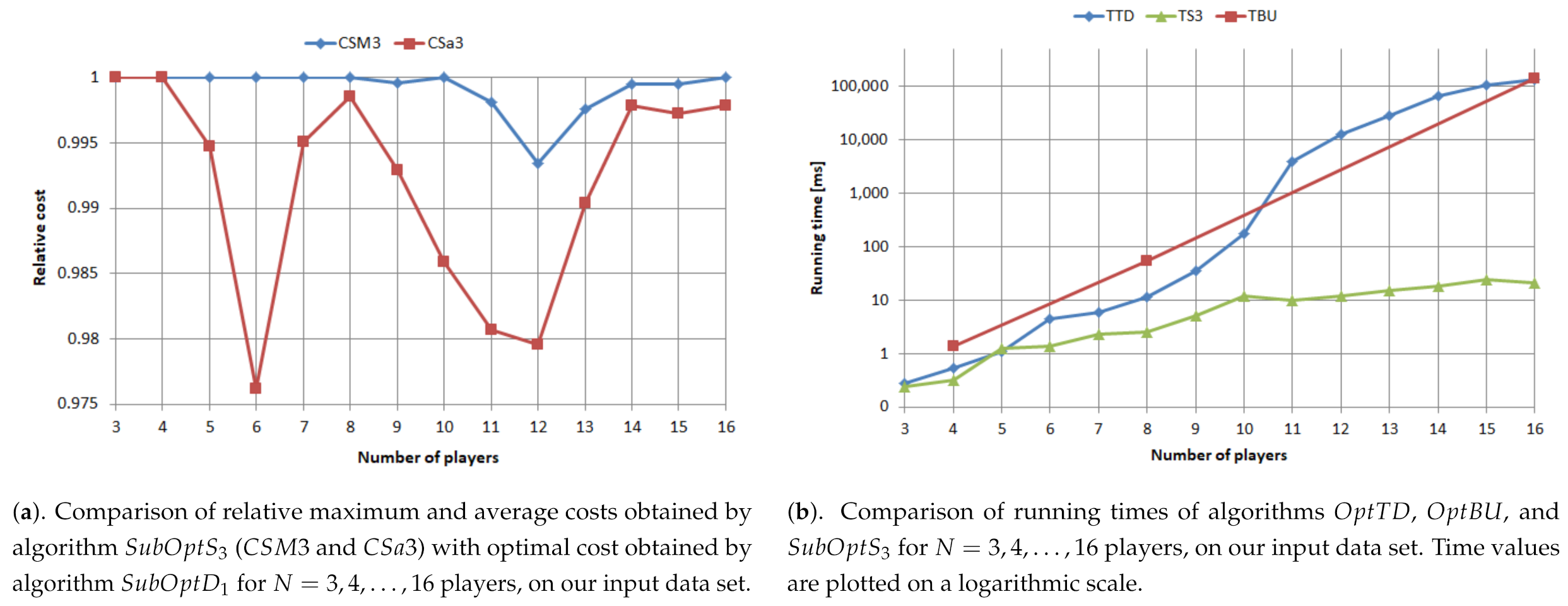
Figure 7 presents results obtained with optimal algorithms $OptTD$ and $OptBU$, as well as their comparison with results obtained by sub-optimal algorithm $SubOpt{S}_3$ for $N=3,4,\dots ,16$ players, on our input data set.

Figure 7. Comparing costs and running times of our implemented algorithms.

In Figure 7a we show the comparison of relative maximum and average costs obtained by algorithm $SubOpt{S}_3$ ($CSM3$ and $CSa3$) with the actual optimal cost obtained by algorithm $OptTD$. The relative sub-optimal cost is a measure $C_r\in (0,1]$ computed with Equation (42) using the absolute values of sub-optimal cost $C_0$ and optimal cost $C_1\ge C_0>0$. Observe that $C_r=1$ if and only if $C_1=C_0$, i.e., if the algorithm providing sub-optimal cost $C_0$ is in fact optimal. Note that the computation of the relative sub-optimal cost assumes the the exact value $C_1$ of the optimal cost is known. In our case, this value is known, as it was determined using the $OptTD$ optimal algorithm for $N=3,4,\dots ,16$ players.

$$C_r=\frac{C_0}{C_1}$$

(42)

In Figure 7b we show the comparison of running times $TTD$, $TBU$, and $TS3$ of algorithms $OptTD$, $OptBU$, and $SubOpt{S}_3$ for $N=3,4,\dots ,16$ players. The running times were evaluated by repeating the algorithm execution 10 times for the same input data. They are plotted on a logarithmic scale. Observe that by far the most efficient among them is algorithm $SubOp{t}_3$. The linear increasing trend of $TTD$ and $TBU$ on the logarithmic scale is consistent to our findings that the complexity of algorithms $OptTD$ and $OptBU$ is exponential with the number of tournament players. Note that this tendency is also observed on the plot of $TBU$, for which the values were recorded only for an exact power of two of the number of players, i.e., $N=4,8,16$. Moreover, the sub-linear increasing trend of $TS3$ on the logarithmic scale is consistent with the fact that algorithm $SubOp{t}_3$ has a polynomial time complexity.

7. Conclusions

In this paper we defined optimal competitions structured as hierarchically shaped single-elimination tournaments. The optimality criterion aimed to maximize tournament attractiveness by letting the topmost players meet in higher stages of the tournament. We proposed a dynamic programming algorithm for computing optimal tournaments and we provided a thorough analysis of its correctness and computational complexity. Based on the idea of the dynamic programming approach, we also developed deterministic and stochastic sub-optimal algorithms. We realized an experimental evaluation of the proposed algorithms by providing experimental results that we obtained with their Python implementation. The results addressed the optimality of solutions and the efficiency of the running time.