1. Introduction
Berrut [
1,
2,
3] introduced two versions of a univariate rational interpolation procedure that has proven to be efficient and effective, even for equally spaced points in an interval. Of note is that the complexity of these procedures is
linear in the number of points. The derivation of these procedures is based on the classical Whittaker–Shannon sampling theorem [
4,
5,
6]).
Theorem 1. Suppose that and that for . Thenwhere, as usual,is the sinc function. In the case of
f with domain restricted to some compact subinterval of
say to
considering equally spaced points with
we may consider the partial sum
where we have set
.
Figure 1 shows a plot of the approximant
and
of the function
where it is evident that when increasing
n the quality of the approximation improves.
While (
2) no longer reproduces
f for all
it is an
interpolant in that
as easily follows from the cardinality property of the translated sinc functions, i.e.,
This interpolant
was already studied by de la Vallée Poussin (1908) who showed that under some weak regularity conditions on
with error essentially of
. The reader interested in further details may find them in the excellent survey by Butzer and Stens [
7].
In order to alleviate the poor approximation quality of
, Berrut in [
2] suggested normalizing the Formula (
2) for
to obtain what we refer to as the
first Berrut rational interpolant:
remains an interpolant of
f at the nodes
but has the advantage of reproducing constants, that is if
then
.
The Formula (
4) may be simplified. Notice that
hence,
An example of this first interpolant is shown in
Figure 2 again for
and
.
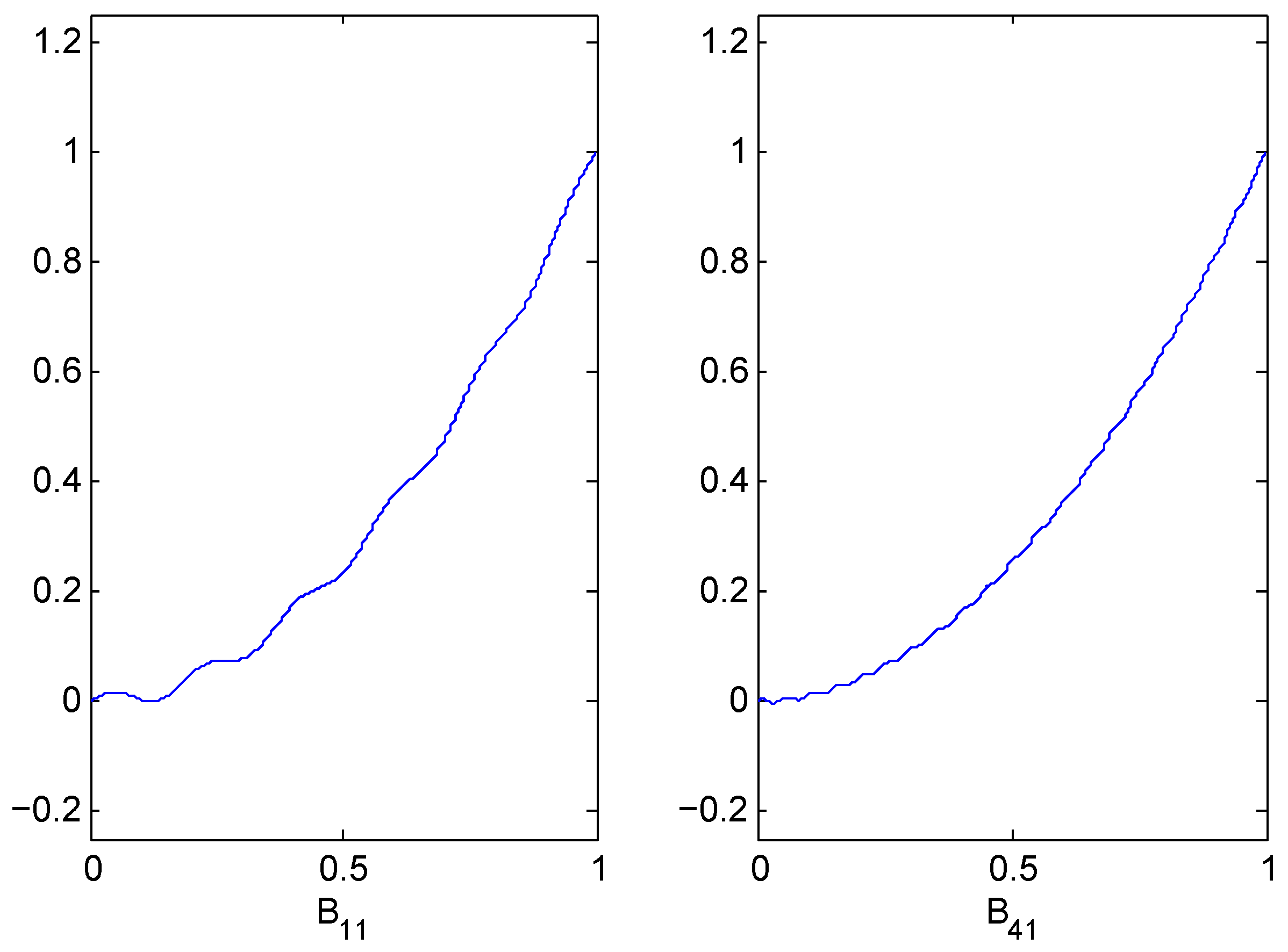
Remark 1. Besides being an improved approximant, is also numerically stable as its associated Lebesgue constant has growth, as was shown in [8]. Berrut also proposed a second improvement by making a simple boundary adjustment in the definition of
to obtain an interpolant that also reproduced polynomials of degree one. Specifically, let
where
Remark 2. Floater and Hormann ([9]) subsequently introduced the more general formulawhere the weights are chosen so that reproduces polynomials of degree at most d In the specific case of equally spaced nodes their formula for the reduces towhere , by assumption. The cases of correspond to Berrut’s first and second interpolants, respectively.
In this work we will consider bivariate extensions of Berrut’s first and second interpolants. The more general Floater-Hormann case will be the topic of a subsequent paper.
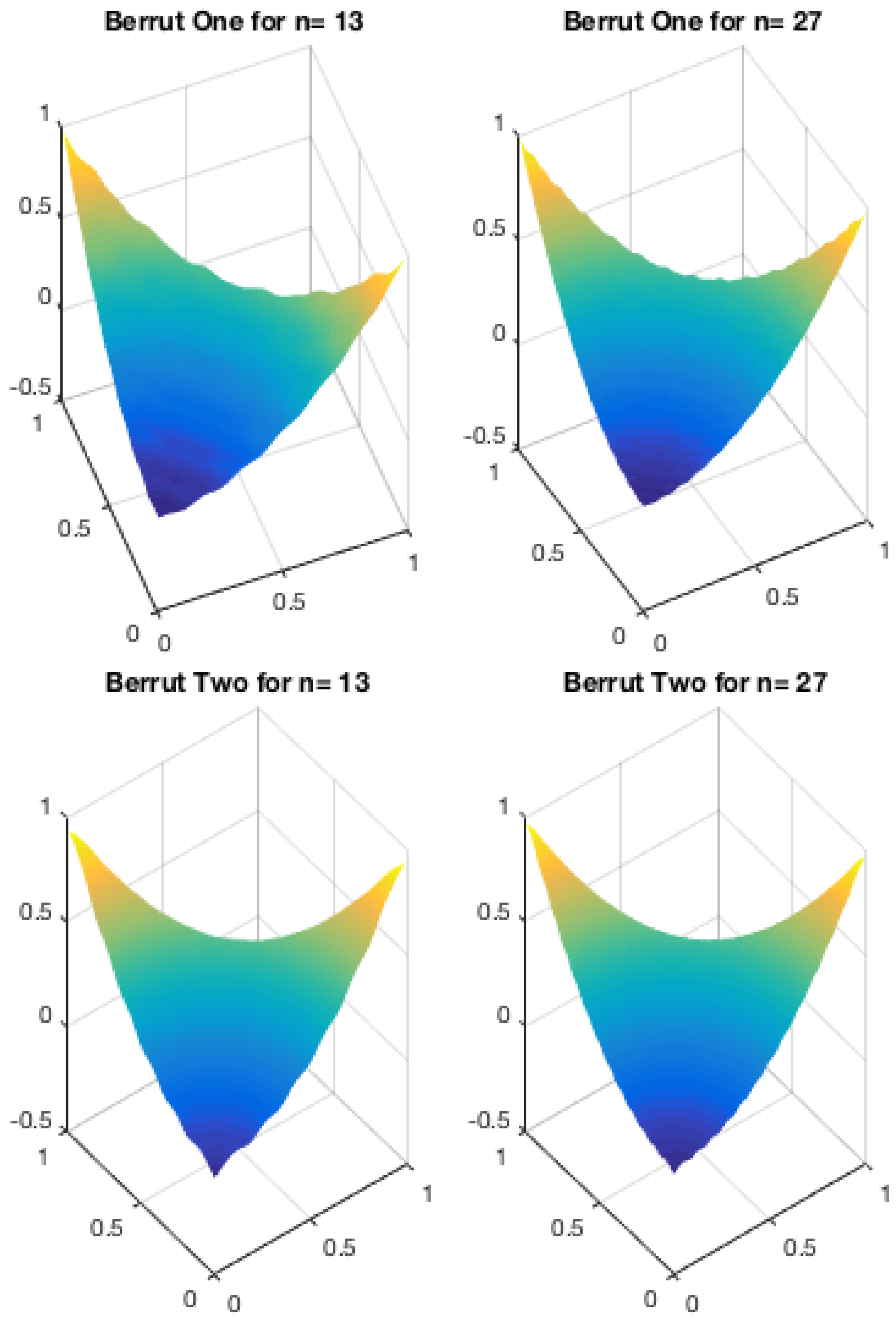
In
Figure 3 we show a comparison between the Berrut interpolants for
and
.
2. The Extension of Berrut’s First Interpolant to Equally Spaced Points on a Triangle
The bivariate Whittaker–Shannon sampling operator is defined as follows. Set
and
then
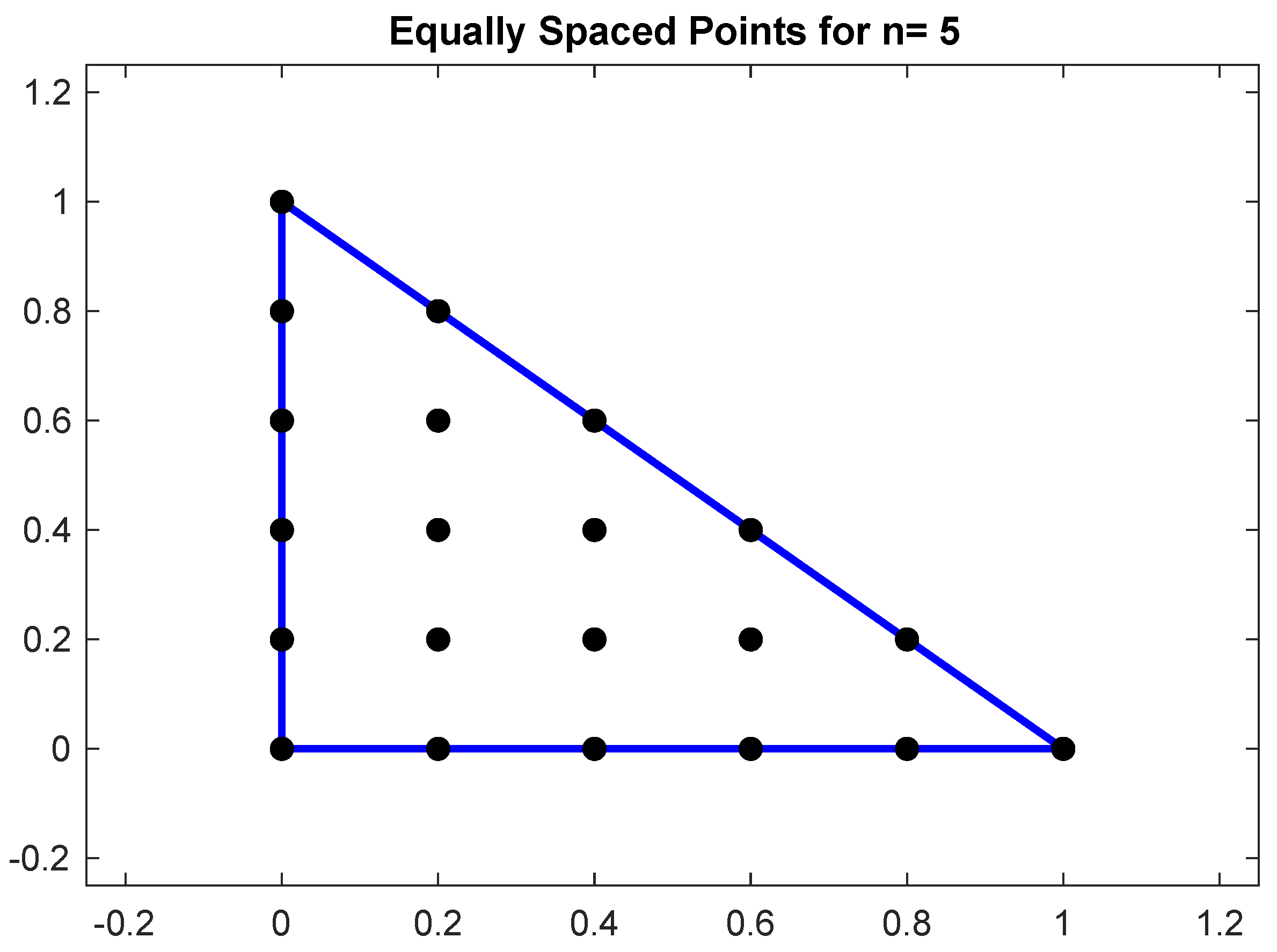
We can now truncate
triangularly (this is equivalent to consider equally spaced points on the triangle, as illustrated in
Figure 4). Let
be the standard triangle in
and set
Furthermore, by normalizing as in the one-dimensional Berrut case, we get
Finally we simplify, just as in the univariate case, to get
Remark 3. Of course the summation can be truncated to regions P other than just the triangle to obtain multivariate versions of the Berrut rational interpolation at integer lattice points contained in P. However, we consider in this first work only the case of a triangle.
Proposition 1. We have that is an interpolant, i.e.,and that reproduces constants. Moreover, restricted to the vertical grid lines and horizontal grid lines agrees with the univariate Berrut interpolant for the interpolation points along those lines. Proof. It is easy to verify these properties. Interpolation is guaranteed by the singularities at the interpolation points while the reproduction of constants is self evident.
To see the grid line first rationalize by multiplying the numerator and denominator by
where
to obtain
Restricting, for example to the vertical grid line
we obtain
However the product
unless
. Hence
which is exactly the univariate Berrut interpolant for the function
along that the line
. □
Remark 4. The restriction of to the upper edge is not a univariate Berrut interpolant, as is easy to confirm. It follows that is not symmetric with respect to the barycentric coordinates of the triangle.
As we have seen, the formula (
11) can be rationalized by multiplying the numerator and denominator by
where
Indeed, writing
let
be the resulting polynomial for the denominator in (
11). The zeros of
correspond to poles in the expression for
and are obviously problematic. We conjecture however that there are no poles
inside the triangle, but have been able to prove this only for
to date. We remark that although the univariate arguments used by Berrut (and more generally by Floater and Hormann) do extend easily to the tensor product case, they do not, to the best of our knowledge, extend easily to the triangular case which we are considering.
Our method to do this is elementary, but computationally expensive. Consider first the
case. Then
Clearly
for
but this can also be confirmed by the use of barycentric coordinates. Indeed, let
so that
. In particular, the triangle
T is given by
Then, homogenizing and simplifying we have
As all the coefficients of are non-negative, it follows that on the interior of the triangle T. By, the previous proposition, we know that there are also no boundary poles on the edges and . The upper edge () needs to be checked separately, which is easily done.
For higher degrees
n it is convenient to change variables letting
so that
where
Then, ignoring the
factor and, by an abuse of notation, suppressing the primes,
a polynomial of degree 4. It can be homogenized to
which becomes, upon setting
(
in barycentric coordinates),
Not all the coefficients are non-negative and hence we cannot immediately conclude that
on
T. However, we may degree elevate this expression, i.e., multiply by a factor
(cf. e.g., [
10]). If it is the case that all the coefficients of the product
are non-negative, it follows that
on
T. (The lowest power
r with this property is related to the so-called
Bernstein degree of .) In this case, consider what occurs if
. Then
The minimum non-zero coefficient, 1 in this case, provides a
certificate of positivity for
on the
interior of
T (where
). Separate certificates for the boundary can be obtained by setting
and
respectively. However, as already noted, the restrictions of the bivariate interpolant to the edges
and
are the univariate Berrut interpolants and hence have no poles there. The upper edge
needs to be done separately.
By these means we may, with the assistance of a computer algebra system, prove the following positivity result.
Proposition 2. For at least Proof. We produced a positivity certificate for the stated values of n using the Matlab Symbolic Toolbox and the following code.
The minimal values of degree elevation are shown in
Table 1.
Notice that the minimal elevation degree r grows quite quickly with n. In principle one can continue with this procedure proving positivity for one degree n at a time. A general proof evades us for the time being. □
In the univariate case it is known that in fact there are no real poles whatsoever. In contrast, in the bivariate case there are real poles, however, due to Proposition 2 they are necessarily outside the triangle.
Proposition 3. For any set of weights the denominatorhas real zeros at for and . Proof. Notice that
However, for
we must have
for all
with
i.e., either
or
(or both). Hence at least one of the products
must be zero, and thus
. □
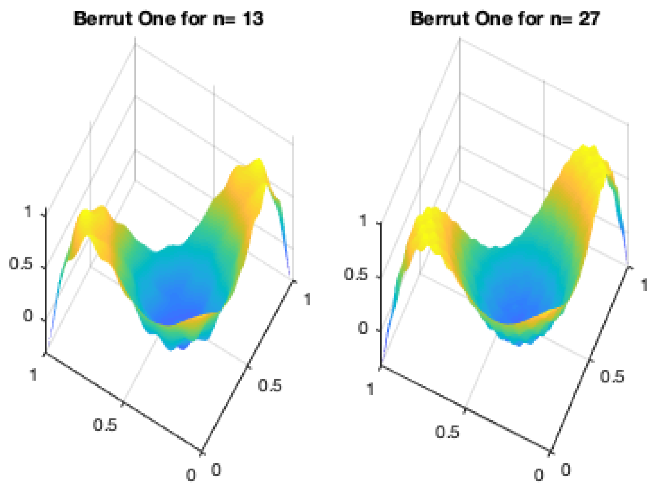
Remark 5. While there are no real poles in the univariate case, there are complex poles. Figure 5 shows these poles for degree . In fact it is possible to analyze the asymptotics of these poles. Indeed, it was shown in [4] thatwhere is the so-called Bateman G-functionLetting we obtainHowever, notice, from the defining formula, thatso that the zeros of are aysmptotically the zeros of divided by n. In particular, one may find numerically thatis a zero of and hence is approximately a zero of . Consequently, in the univariate case, there are complex poles of distance order to the interval whereas in the bivariate case there are real poles of this same order of distance to the triangle T. Finally, we show some examples of this bivariate interpolant.
Figure 6 shows the bivariate extension of Berrut’s first interpolant for the function
and
.
Figure 7 shows the interpolant of
for the same degrees.
One may notice that the interpolant is reasonable for higher values of n but leaves room for improvement.
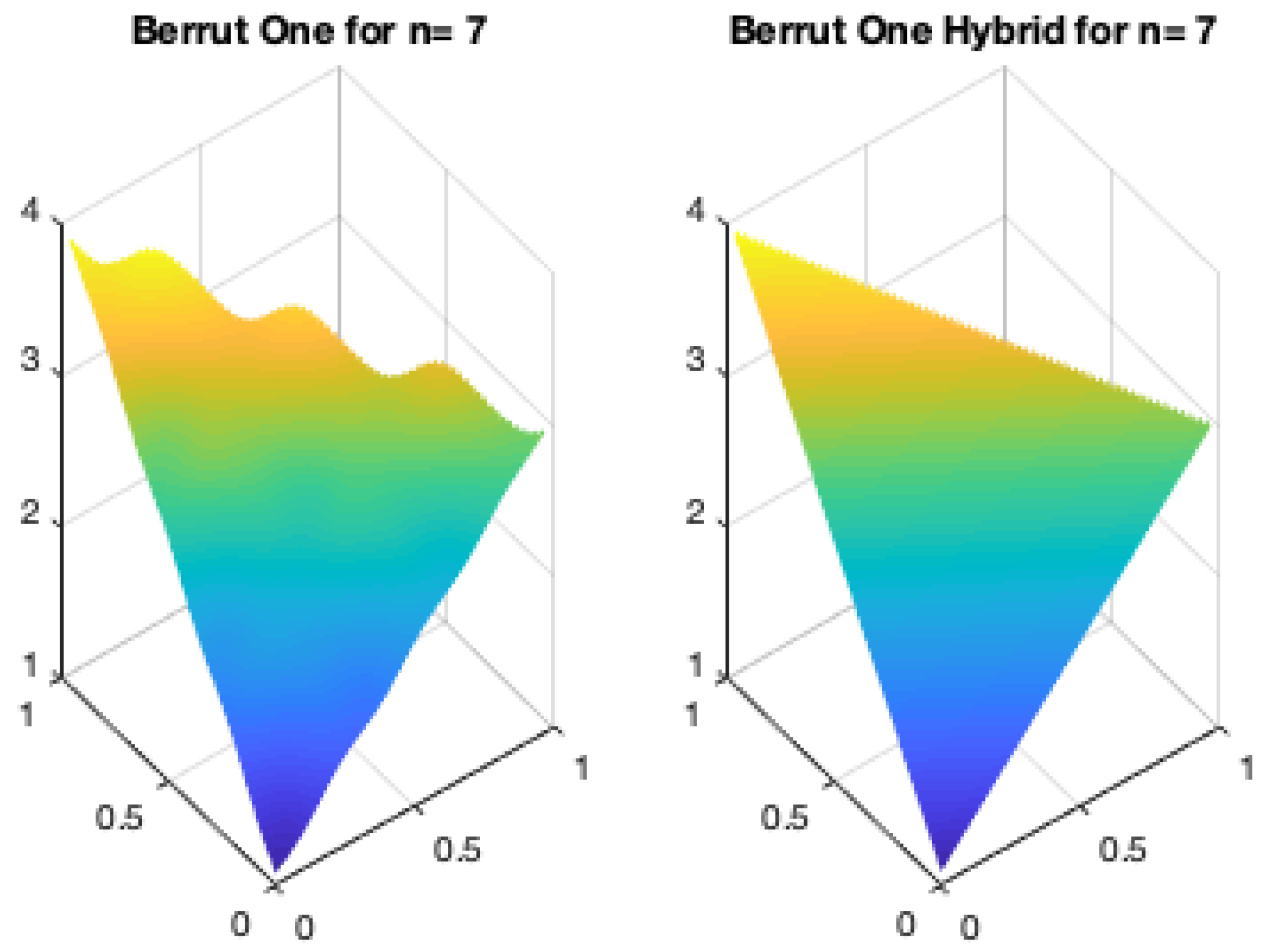
A Hybrid Interpolant
For any linear interpolant it is possible, by means of a so-called Boolean sum, to create a hybrid version that reproduces any specifed finite dimensional subspace of functions, the most common example of such being the space of polynomials of degree one. Indeed, for example, if
denotes the linear interpolant of
f at the three vertices of
i.e.,
then for
we may defined
where
is the interpolant of
.
Figure 8 give a comparison between the original
and its hybrid version, for
and
.
3. The Extension of Berrut’s Second Interpolant to Equally Spaced Points on a Triangle
Berrut’s second interpolant (for when the boundary points are included) involves the introduction of weights, adjusted at the boundary, to ensure the reproduction of linears. In general, for weights
we define
In the bivariate case the reproduction of linears splits into
n odd and
n even cases. We consider first the
n odd case for which we define the weights
(i.e., 0 at the three vertices,
at the interior edge points and 1 at the triangle interior points). The
case is shown in
Figure 9.
Proposition 4. For odd and weights given by (13), reproduces polynomials of degree one. Proof. We remark that the case has all weights zero, and hence is not relevant. □
We will make use of univariate reproduction formulas for Berrut’s second interpolant.
Lemma 1. For any points and weights if and only if Lemma 2. Consider the weightswith a parameter. Then for and any or and m odd Proof. By Lemma 1 we need only show that .
The
case is the result first proved by Berrut and hence we leave out the details. In case
and
m is odd then we calculate
as this is an alternating sum of
with an even (
) number of terms. □
Now to prove Proposition 4. We wish to show that
for any
. Clearly it suffices to show this for
which we now proceed to do. First note that, by scaling by a factor of
n this is equivalnet to showing that
Now write the summation by rows as
For the first row,
the weights correspond to the lower edge and are
and we apply the univariate Lemma with
and
to obtain
For the other rows,
the weights are
and we may apply the univariate Lemma with
and
to obtain
For the top row (actually a singleton),
and so there is nothing to do. □
Remark 6. The zero weights at the vertices means that will not interpolate at those points. It will however provide an order approximation to the corresponding value of f, provided it is minimally smooth. The approximation properties of these interpolants will be discussed in a forthcoming work.
Just as in the first interpolant case, by Lemma 3, there are poles at . However, just as in the first case, there are no poles in the triangle T.
Proposition 5. For at least Proof. We do this in exactly the same manner as in the first case, by using degree elevation to produce a positivity certificate, one degree at a time. The minimal values of degree elevation are displayed in
Table 2. □
The n even case splits into two subcases.
n, A Multiple of Four
In case
n is a multiple of four we introduce the weights of 1 at interior points and along each edge
where the
bracketed by
to the left and right is the middle entry,
(
Figure 10).
We first remark that in the univariate case the rational interpolant with these weights, for n a multiple of four, reproduces linears.
Lemma 3. For n a multiple of four and the weights given by (14), Proof. Applying Lemma 1 we calculate
and the result follows. □
Proposition 6. For the weights given by (14) and n a multiple of four, the Berrut two extension reproduces linears. Proof. We will show that
for any
. Again, it suffices to show this for
i.e., that
We again proceed row by row. The bottom row
is the case discussed in Lemma 3. The other rows, other than for
follow from the
case of Lemma 2. For
we have
Now we claim that
from which the result for the
th row follows. To see this just note that for row
The row
is completely analogous. □
Just as in the previous cases, by Lemma 3, there are poles at . However, we conjeture that there are no poles in the triangle T.
Proposition 7. For at least Proof. We do this in exactly the same manner as before, by using degree elevation to produce a positivity certificate, one degree at a time. The minimal values of degree elevation are displayed in
Table 3.
This concludes the proof. □
Figure 11 shows the result of interpolating
for
and
.


