Incremental DoE and Modeling Methodology with Gaussian Process Regression: An Industrially Applicable Approach to Incorporate Expert Knowledge

Abstract

The use of data-based models is a favorable way to optimize existing industrial processes. Estimation of these models requires data with sufficient information content. However, data from regular process operation are typically limited to single operating points, so industrially applicable design of experiments (DoE) methods are needed. This paper presents a stepwise DoE and modeling methodology, using Gaussian process regression that incorporates expert knowledge. This expert knowledge regarding an appropriate operating point and the importance of various process inputs is exploited in both the model construction and the experimental design. An incremental modeling scheme is used in which a model is additively extended by another submodel in a stepwise fashion, each estimated on a suitable experimental design. Starting with the most important process input for the first submodel, the number of considered inputs is incremented in each step. The strengths and weaknesses of the methodology are investigated, using synthetic data in different scenarios. The results show that a high overall model quality is reached, especially for processes with few interactions between the inputs and low noise levels. Furthermore, advantages in the interpretability and applicability for industrial processes are discussed and demonstrated, using a real industrial use case as an example.

1. Introduction

Modern industrial companies are facing several challenges that are caused by legislation and the market. Key factors for economic success are continuous improvements in product quality, resource efficiency and productive time. Since production lines are typically operated for decades, methods for improving such existing industrial processes are needed. These improvements could be, for example, to determine the optimal process parameters for an individual product or to predict a need for maintenance of a production plant [1]. To do this, two basic types of models can be distinguished. On the one hand, first principles models can be used, which possess a high area of validity but require in-depth knowledge of the regarded system. On the other hand, data-based models can be used, which can be estimated with less knowledge, for example, by applying machine learning techniques, but heavily rely on the available data. Due to the high complexity of real-world processes and missing insight, the creation of the first principles models is often inapplicable, and thus, data-based models are preferred. However, collecting representative data sets for model estimation is a challenging task for real-world industrial processes. These challenges include the availability of data, variations of external influences on a process and the detection of system boundaries [2].

As stated in [3], design of experiments (DoE) methods are helpful to support the creation of machine learning models in real industrial environments, for example, by identifying relevant features used as model inputs. If no continuous process monitoring is available, DoE methods can be used to create suitable data sets for model estimation with reasonable effort. Furthermore, industrial processes are typically operated in few fixed operating points. Even if a process is monitored continuously and a huge amount of data is available, data distribution might be unsuitable for model estimation. Such a data distribution is schematically depicted in Figure 1 for an industrial process with a single operating point in a two-dimensional input space.

As shown, data points are mainly concentrated around the given operating point. Due to normal process variations, an operational area surrounding the operating point is given in which data can be observed. As the operational area covers only parts of the input space, the validity of a model estimate on these data is limited. In particular, such a model is inappropriate to determine an optimum outside this operational area due to extrapolation, which is exemplarily shown in Figure 1. For gathering information in all relevant parts of the input space, DoE methods are needed that take additional requirements of industrial processes, such as constraints in the input space, into account. Such constraints are exemplarily shown in Figure 1 and define the borders of the feasible input region. Design points must only be placed inside this region to avoid abnormal process behavior or even defects of the process equipment. Applying DoE methods to industrial processes heavily relies on domain knowledge. Typically, experiments are planned by an interdisciplinary team and are executed sequentially in order to gain additional information that supports the next experiment [4]. A critical step in this procedure is the specification of the regarded factors. This specification requires in-depth knowledge or special screening experiments [5]. In case of doubt, an input will be included in the experiment, leading to higher dimensionality of the design space, which increases the required number of data points and the measurement effort.

To overcome these issues, this paper presents a stepwise DoE and modeling methodology called incremental Latin hypercube additive design (ILHAD) in which the dimensionality of the design space does not need to be predefined. Instead, in each step, one new input is incorporated into the experimental design. All inputs regarded in the experimental design are varied systematically, whereas all remaining process inputs are fixed to the value of a given operating point. By previously sorting all inputs according to the expected influence on the process output, data containing the main functional relationships are gathered in the first steps. Data from every step are then used to estimate a new submodel that models the main effects of the newly added input and the interactions with all already regarded inputs. By additively superposing all available submodels, the overall process model is built. The benefits of this methodology were shown in [6] in combination with local linear model trees as the submodel structure. For constructing this type of submodel structure, the input space is successively partitioned. The process behavior in each partition is mainly modeled by a corresponding local linear model. As the parameters of these local models need to be estimated, sufficient data points in each partition must be present. To achieve a high model quality, a strategy for increasing the point density in specific parts of the input space, based on information from previous ILHAD steps, was proposed. In this work, the submodels are created, using Gaussian process regression (GPR), which is a non-parametric regression model. In this way, a flexible model structure is given, enabling the modeling of nonlinear processes. GPR models offer a high model quality, even on a low number of training data points, which makes them well suited for an application on designed experiments.

In terms of the information content of the gathered data and the measurement effort, Figure 2 compares between process observation, ILHAD and using a space-filling design, which is one of the classical DoE methods.

As stated before, the information content of data from process observation is typically low because data are often limited to distinct operating points. As no separate experiments need to be performed, this method possesses the lowest measurement effort. Using space-filling design methods, a high information content can be achieved by gathering data over the whole input space. However, in-depth process knowledge is required in advance to check the feasibility of all design points and to select all inputs that span the design space. ILHAD aims to reduce the measurement effort by applying stepwise experiments in a design space with increasing dimensionality. This leads to a low complexity of the measurement procedure and the process model in the first steps, which enables an intuitive understanding of the process behavior and supports the incorporation of expert knowledge. Concerning this methodology, the following research questions are addressed:

• What benefits in the applicability of DoE methods for industrial processes can be achieved using the proposed method?
• What model quality can be achieved by the incremental modeling methodology, compared to a classical DoE and modeling method?
• How can expert knowledge be used to support the experimental design and modeling process?

The remainder of this paper is organized as follows: Section 2 reviews related work concerning DoE approaches for industrial applications, additive model structures and stepwise DoE and modeling methodologies. In Section 3, the proposed DoE and modeling methodology is described with a focus on different modifications of the GPR model to be used in ILHAD. Results from a computer simulation experiment and a real-world industrial process are presented in Section 4. In Section 5, the obtained results are discussed with respect to the stated research questions. Finally, concluding remarks are given in Section 6.

2. Related Work

In this section, related work in the area of additive model structures and DoE methods for industrial applications is presented. As the proposed methodology combines methods from both areas, stepwise DoE and modeling methodologies are reviewed.

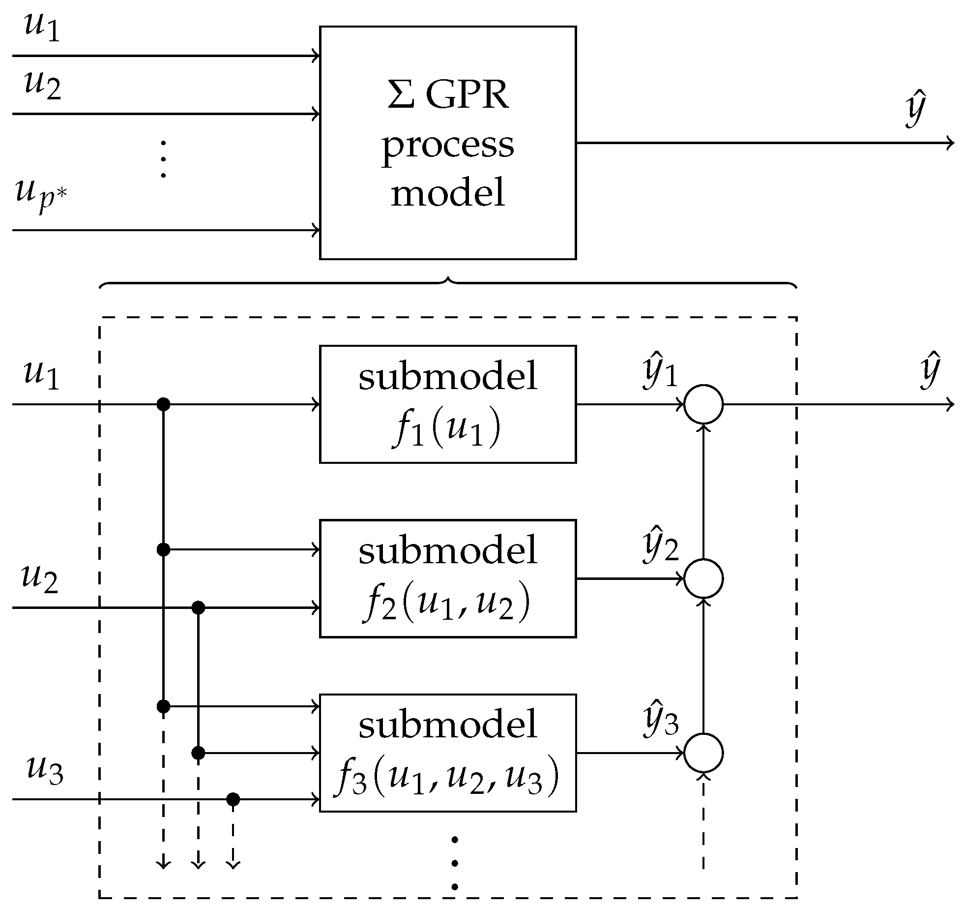
2.1. Additive Model Structures

Additive model structures are a common approach in data-based modeling. An overall process model is created from multiple submodels, which are additively superposed. Typically, simple submodel structures are used, which can be estimated with low computational effort. This computational effort can further be reduced if each submodel makes use of a subset of the given inputs so that a lower-dimensional problem is given [7]. A simple additive model structure is a polynomial regression model in which each regressor depends either on a single input (main effect) or on a combination of different inputs (interactions). This separation of main effects and interactions enables the interpretation of such models [8]. In addition, these models can be estimated with a low computational effort but possess limited flexibility, due to the fixed model structure. By extending a polynomial model with nonparametric functions of the regressors, generalized additive models (GAM) are given, which provide higher flexibility while maintaining the interpretability, due to the separation of the single effects [9]. In [10], a GAM was used for forecasting the heat production of a heat and power plant based on weather data. Due to the GAM structure, an interpretable model was estimated that can be simply validated.

Additive Gaussian processes use a similar strategy to increase interpretability and to achieve a low model error. In [11], a GPR model was trained with an additive kernel function, consisting of a base kernel and kernels for the interactions. Each interaction is weighted by an individual hyperparameter that controls the influence of a specific interaction on the process output. These hyperparameters can be interpreted as a measure of the importance of such interactions.

Additive models that combine different types of models were described in [12,13]. These incremental models consist of a global model and additional local models, which refine the model in nonlinear regions of the input space. For the global model, a linear regression model is suitable, whereas fuzzy models are used as local models for error compensation. Another popular technique that makes use of an additive model structure is boosting, in which an initial model is improved stepwise by additional error models. Each error model is trained on the error of the previous model, for which the sum of squared errors can be used as a loss function. This enables a computationally efficient model fitting by using the least squares method [14]. Even with simple model structures of the additive models, a high overall model quality can be achieved, which is, for example, demonstrated by the state-of-the-art boosting method XGBoost [15].

2.2. DoE for Industrial Applications

An efficient way to create representative data sets for modeling is to make use of DoE methods. Classical experimental designs, such as full factorial designs, examine combinations of factors on distinct levels. With a high number of factors and levels considered, these designs lead to a high measuring effort [16]. In [17], such a full factorial experimental design was applied to a metal cutting process. To achieve an appropriate measurement effort in this use case, the number of regarded factors has to be reduced. Therefore, a prior screening experiment is performed to identify significant factors.

Another class of experimental designs are optimal designs. Compared to full factorial designs, the measurement effort is reduced by selecting design points, according to an optimization criterion. A popular criterion is the D-optimality, which minimizes the determinant of the Fisher information matrix. In this way, the overall variance of the parameter estimates is minimized [18]. An application of such a D-optimal design for modeling the surface quality in a turning process is given in [19]. However, optimal designs require a specification of the model structure prior to the measurements. The generalization error of a model is composed of bias and variance error. As the variance error can be minimized by an optimal design criterion, the bias error is caused by the assumed model structure. If a chosen model structure is not flexible enough for the modeled functional relationship, this leads to a high bias error [20].

A popular way to overcome this issue is to make use of a flexible model structure in combination with regularization techniques, such as ridge regression or lasso [21]. These techniques use a penalty term in the loss function to reduce the number of effective parameters in a model. In this way, even the very flexible model structure of Gaussian process (GP) models, which possess as many parameters as training data points, can be used without overfitting [22]. To estimate such GP models, space-filling designs are typically used, which evenly spread design points over the input space [18]. This type of uniform space-filling designs can directly be used if little knowledge about the functional relationship to be modeled is given. In [23], methods for creating non-uniform space-filling designs are presented, which make use of expert knowledge. These methods include an individual scaling of the inputs to reflect the assumed effect of an input on the process output and an increased point density in important regions of the input space by assigning weights.

All previously discussed experimental designs require the number of data points to be determined in advance, which is a nontrivial task and heavily affects the model quality and the required measurement effort. Sequential designs, in which an overall design is created in multiple steps, do not possess this drawback [24]. These designs enable efficient strategies to reduce the computational effort for optimizing a design, for example, by constructing nested designs in high-dimensional spaces [25]. Furthermore, the knowledge gained in previous steps is available, which can be used to improve the design in the next step. Such techniques in which additional points are placed in regions of interest in the input space, such as regions close to a predicted location of an optimum, are called augmentation [26]. Sequential designs are closely related to the concept of active learning. In active learning techniques, informative data points are selected, according to a criterion based on the model trained so far. Active learning strategies can be divided into stream-based active learning in which a measurement decision is made for each point in a data stream, and pool-based active learning in which a set of informative points is selected from a large set of points [27]. Active learning approaches have successfully been used for modeling industrial processes. For example, in [28] a soft sensor for a penicillin fermentation process was developed, which achieves a high prediction accuracy and a low measurement effort compared to a classical approach.

2.3. Stepwise DoE and Modeling Methodologies

Classical DoE strategies are intended to be executed only once. However, in practice multiple experiments with different design strategies are typically performed so that more process knowledge is gained in each experiment. These experiments might fulfill a special purpose, such as identifying relevant inputs in a screening experiment, or might aim to model the process with an assumed model structure [16]. Choosing a suitable sequence of experimental design methods for a specific industrial use case is a challenging task. Instead, stepwise methods, with an increasing complexity of the models and the measurement procedure, enable to execute as many steps as required with a clear strategy.

In [29], a stepwise methodology for creating high-order polynomial surrogate models was presented. It makes use of Chebyshev polynomials as a model structure, which are newly estimated in each step. Additional training data points are selected stepwise from a space-filling design based on the current model. To reach a higher accuracy, the order of the Chebyshev polynomial is incremented in each step until a termination criterion is met. A similar approach for the identification of dynamic systems was described in [30]. A procedure with alternating DoE and modeling steps is applied. It makes use of polynomial nonlinear state space models in combination with D-optimal designs. In each step, a new model with an incremented polynomial is estimated in order to improve the model quality.

3. Materials and Methods

The preceding brief literature review reveals that additive model structures are widely used and are beneficial in terms of interpretability. In addition, a broad variety of DoE methods exists, but most classical DoE methods either require in-depth knowledge of the functional relationship to be modeled or make use of measurement procedures that cause a high effort in real industrial processes. To apply DoE methods in practice, confidence needs to be built so that the plant operators are willing to take the risk of performing experiments. Stepwise experiments with increasing complexity are one way to create this confidence. In combination with process model structures composed of multiple submodels, a stepwise exploration of process behavior can be achieved, providing both a simplified measurement procedure and an increased understanding of the functional relationships of the process.

The regarded industrial process possesses p different inputs $u_1,u_2,\dots ,u_p$ and one output y and should be modeled by a static process model. The basic activities of the proposed DoE and modeling methodology to create such a model are depicted as a flowchart in Figure 3.

Real industrial processes usually have inputs that vary in importance. Some inputs strongly influence the process, while the effects of some inputs might even be neglected. As an initial activity in the methodology, all available process inputs are ranked, according to their expected influence on the process output. These inputs are arranged in descending order of relevance in the input vector $\mathbf{u}=[u_1{u}_2\dots u_p]$, so that $u_1$ is the most important input. All remaining activities of the methodology are performed in $p^{*}\le p$ steps. In each step $i\in \{1,2,\dots ,p^{*}\}$, the next important input $u_i$ is used to expand the design space so that its dimensionality increases. To gather information over the whole newly regarded design space, a new space-filling design ${\mathcal{D}}_i$ is created in each step. For that purpose, several design strategies are suitable. As an example, uniform designs [31] that minimize the discrepancy between the uniform distribution and the distribution of the design points can be effectively used for stepwise experiments [32]. The threshold accepting algorithm [33] and adjusted threshold accepting algorithm are widely used algorithms for constructing this type of design. In the following, an optimized Latin hypercube (LHC) design is used, which provides good space-filling and projectional properties. These projectional properties ensure that a space-filling design is still given if inputs are irrelevant [34]. Next, the design points in ${\mathcal{D}}_i$ are used in an experiment to gather data from the process. All inputs $u_{i+1},u_{i+2},\dots ,u_p$ that are not specified by the design are fixed to the values of a given operating point $\overline{\mathbf{u}}=[{\overline{u}}_1{\overline{u}}_2\dots {\overline{u}}_p]$. The obtained measurements in this step are then used to estimate a new submodel $f_i$, which models the main effect of the newly added input $u_i$ and the interactions with all previously regarded inputs $u_1,u_2,\dots ,u_{i-1}$. All estimated submodels are superposed to create an overall process model, which contains all main effects and all interactions of all inputs regarded so far. GPR is used as the internal model structure of each submodel, enabling the modeling of nonlinear process behavior, due to its high flexibility. As these submodels are estimated one after another on a relatively small data set, the parameter estimation is simple and the computational demand is low. The methodology can be terminated after every step so that the number of steps $p^{*}$ does not have to be predefined. Instead, a required model quality or available measurement time can be used as a termination criterion. Hereafter, the single activities of the methodology are described in more detail.

3.1. Incremental Models

In ILHAD, an additive model structure, which is shown in Figure 4, is used to create the overall process model.

An overall process model in step i consists of i different submodels, which are created one after another. By summing up all outputs of the submodels ${\widehat{y}}_j$ the overall model output is calculated as follows:

$$\widehat{y}=\sum _{j=1}^i{\widehat{y}}_j=\sum _{j=1}^i{f}_j({\mathbf{u}}_j)$$

(1)

Each submodel $f_j({\mathbf{u}}_j)$ in the additive structure makes use of a subset of inputs, which is described as an individual input vector ${\mathbf{u}}_j=[u_1{u}_2\dots u_j]$. The main construction principle of an increasing input dimensionality is related to [35] in which such an approach is applied to neural networks. In each step, a new neural network is trained, incorporating additional inputs. All networks are then merged together to create an overall process model. In this way, new functional relationships can be incorporated into the model without retraining the whole model.

In ILHAD, each submodel is estimated on the basis of an individual experimental design ${\mathcal{D}}_i=\{\mathbf{x}(1),\mathbf{x}(2),\dots ,\mathbf{x}(N_i)\}$ with $N_i$ design points. The designs are created using the construction mechanism described in Section 3.2. Each design point $\mathbf{x}(k)=[u_1(k)u_2(k)\dots u_i(k)]$ with $k=1,\dots ,N_i$ contains input values for all i inputs regarded so far. All remaining $p-i$ process inputs are fixed to the corresponding coordinates of the operating point ${\overline{\mathbf{u}}}_{p-i}=[{\overline{u}}_{i+1}{\overline{u}}_{i+2}\dots {\overline{u}}_p]$. The composition of the process input vector $\mathbf{u}=[u_1{u}_2\dots u_i{\overline{u}}_{i+1}{\overline{u}}_{i+2}\dots {\overline{u}}_p]$ from the experimental design and the operating point is depicted in Figure 5.

In addition, the calculation of the output value ${\tilde{y}}_i=y-y_{\Sigma }$ that should be modeled by the submodel $f_i$ is shown. Each submodel is trained to model the difference between the measured process output y and the already modeled process behavior, given by the sum of all existing model outputs $y_{\Sigma }={\sum }_{j=1}^{i-1}{\widehat{y}}_j$. As each submodel is a GPR model, which is linear in the parameters, the least squares method can be used for parameter estimation, which leads to a minimization of the quadratic model error $e_i^2={({\tilde{y}}_i-{\widehat{y}}_i)}^2$ in each step. For the process to be modeled, additive white Gaussian noise $n\sim \mathcal{N}(0,{\sigma }_{\mathrm{n}}^2)$ at the process output is assumed.

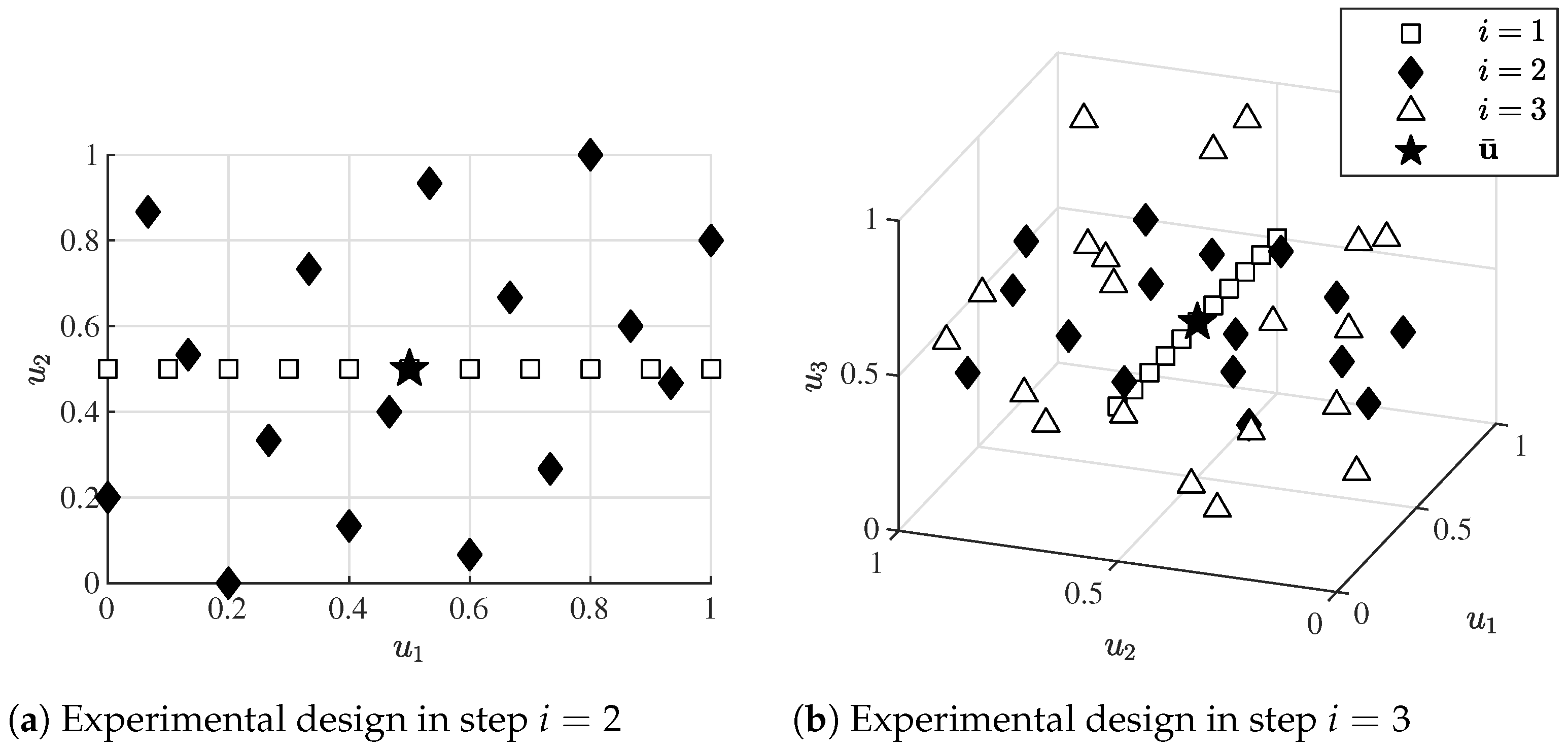
3.2. Experimental Design

In each step of ILHAD, a suitable experimental design is needed to gather data for estimating a new submodel $f_i$. Each of these designs must provide as much information on the main effects and interactions of the newly added input as possible with manageable measurement effort. Due to the composition of the process input, depicted in Figure 5, the dimensionality of the regarded input space is incremented step by step, starting with the one-dimensional input space of $f_1$. As the hypervolume of the input space grows exponentially with increasing dimensionality, an exponentially increasing number of data points would be needed to maintain a desired point density in the input space (curse of dimensionality) [36]. As this exponentially increasing number of points leads to a high measurement effort that is impracticable for real industrial processes, the number of data points must be limited. Due to the ranking of the inputs, the first regarded inputs are most important for the overall model quality, whereas the influences of further inputs can be modeled more roughly. Consequently a decreasing point density with growing dimensionality of the input space can be accepted if the difference in importance of the single inputs is large enough. Various strategies for determining the number of design points in each step are possible, which reduce the measurement effort, compared to the exponential case. In the following, a constant and a linear increasing number of data points are used, which are determined empirically. In general, the number of points can also be specified based on domain knowledge. For example, a higher number of data points can be assigned to steps in which strong nonlinearities or strong interactions of the inputs are expected. The numbers of data points in each incremental design are summarized in the vector $\mathbf{N}=[N_1{N}_2\dots N_{p^{*}}]$.

In addition to the number of design points, the type of design must be specified. As, typically, little prior knowledge on the exact functional relationship of the regarded process is given, space-filling designs are used in every step of ILHAD to gather information over the whole regarded input space. An optimized LHC design is a common type of space-filling design, which is used in the following. A LHC with $N_i$ data points divides each axis into $N_i$ equally spaced levels. Design points are placed such that each level on each axis is only assigned once to a design point. LHC can be easily constructed with an arbitrary number of design points and dimensionality, but require an optimization to ensure good space-filling properties [37]. For the optimization different criteria can be used, which are discussed in [34]. In the following, the maximin criterion is used:

$$\underset{{\mathcal{D}}_i}{max}(d_{\min })=\underset{{\mathcal{D}}_i}{max}\left(\underset{\mathbf{x}(k),\mathbf{x}(l)\in {\mathcal{D}}_i,k\ne l}{min}\left(d(\mathbf{x}(k),\mathbf{x}(l))\right)\right),$$

(2)

leading to a maximization of the minimal point distance $d_{\min }$ in a design ${\mathcal{D}}_i$. The Euclidean distance between two different design points is denoted as $d(\mathbf{x}(k),\mathbf{x}(l))$. Starting from a random LHC, an optimization is performed by the extended deterministic local search (EDLS) algorithm [38], which uses a local search strategy. Each iteration of the algorithm begins with identifying the worst point in the design in terms of the maximin criterion. All other design points are systematically checked as possible exchange partners for a coordinate exchange in one dimension. If such a coordinate exchange leads to an increased minimal point distance in the design, this exchange is executed, and the algorithm proceeds to the next iteration. If no further improvement of the minimal distance in the design is possible, the worst point is temporarily excluded from the determination of the minimal distance. In this way, further minimal distances can be improved, resulting in a more uniform distribution.

The incremental design is constructed by creating optimized LHC designs in an input space with increasing dimensionality. As described in Section 3.1, all inputs that are not yet regarded in the incremental design are fixed to the coordinate of the given operating point. The resulting experimental designs in the second and third step of ILHAD are exemplarily depicted in Figure 6.

To illustrate the construction principle, design points from the previous steps are additionally presented. The one-dimensional LHC in the first step leads to equally spaced points on a straight line parallel to the $u_1$-axis, running through the operating point. All points depicted in Figure 6a are also visible in Figure 6b in the $u_1{u}_2$-plane with $u_3={\overline{u}}_3=0.5$. This means that each design created in step $i-1$ covers a subspace of the input space in step i with $u_i={\overline{u}}_i$. As plenty of data points from this subspace are already available, no additional point must be measured in this subspace. In addition, the used model structure enforces that a point in this subspace would not have any influence on a newly estimated submodel (see Section 3.4).

3.3. Gaussian Process Regression

For each submodel in the incremental model structure, a separate GPR model is estimated on the basis of $N_i$ data points. These data points consist of the design points $\mathbf{x}(k)=[u_1(k)u_2(k)\dots u_i(k)]$ with $k=1,\dots ,N_i$ in ${\mathcal{D}}_i$, each containing a subset of the process inputs, and the corresponding output values $\tilde{\mathbf{y}}={[\tilde{y}(1)\tilde{y}(2)\dots \tilde{y}(N_i)]}^{\mathrm{T}}$ to be modeled.

3.3.1. Fundamentals

GPR models are Bayesian models that use a prior over functions to control the smoothness of the model output. As GPR models are non-parametric, high flexibility is given [22]. A key element to specify the prior is the kernel function $K(\mathbf{x}(k),\mathbf{x}(l))$, which is used as a measure of similarity. It is evaluated on two arbitrary points $\mathbf{x}(k)$ and $\mathbf{x}(l)$ with $k=1,\dots ,N_i$ and $l=1,\dots ,N_i$. A main assumption is that a high similarity of these two points in terms of the kernel function should result in similar output values of the model. As a kernel function, the Gaussian kernel with an Euclidean norm is used as follows:

$$K(\mathbf{x}(k),\mathbf{x}(l))={\sigma }_{\mathrm{f}}^{2}exp\left(-\frac{1}{2}\sum _{m=1}^i\frac{{(u_m(k)-u_m(l))}^2}{{\sigma }_m^2}\right)$$

(3)

This kernel is parametrized by the signal standard deviation ${\sigma }_{\mathrm{f}}$ and an individual length scale ${\sigma }_m$ for each of the i regarded input dimensions. In general, the output values used for model estimation are affected by noise. In the following, the noise-free case $n=0$ is considered first. Based on all input data $\mathbf{x}\in {\mathcal{D}}_i$ the kernel matrix

$$\mathbf{K}=\left[\begin{array}{cccc}\mathrm{cov}\{\tilde{y}(1),\tilde{y}(1)\}& \mathrm{cov}\{\tilde{y}(1),\tilde{y}(2)\}& \dots & \mathrm{cov}\{\tilde{y}(1),\tilde{y}(N_i)\}\\ \mathrm{cov}\{\tilde{y}(2),\tilde{y}(1)\}& \mathrm{cov}\{\tilde{y}(2),\tilde{y}(2)\}& \dots & \mathrm{cov}\{\tilde{y}(2),\tilde{y}(N_i)\}\\ ⋮& ⋮& \ddots & ⋮\\ \mathrm{cov}\{\tilde{y}(N_i),\tilde{y}(1)\}& \mathrm{cov}\{\tilde{y}(N_i),\tilde{y}(2)\}& \dots & \mathrm{cov}\{\tilde{y}(N_i),\tilde{y}(N_i)\}\end{array}\right]$$

(4)

with $\mathrm{cov}\{\tilde{y}(k),\tilde{y}(l)\}=K(\mathbf{x}(k),\mathbf{x}(l))$ is calculated. The kernel matrix describes all covariances between the corresponding model outputs

$$\widehat{\mathbf{y}}={[\widehat{y}(1)\widehat{y}(2)\dots \widehat{y}(N_i)]}^{\mathrm{T}}\sim \mathcal{N}(\mathbf{0},\mathbf{K})$$

(5)

for which typically a zero mean joint normal distribution is assumed. This joint normal distribution of the output is the prior, which determines the smoothness of the model output [7]. For predicting the output value $y_{*}$ for an arbitrary point ${\mathbf{x}}_{*}$ the joint normal distribution is extended to the following:

$$\left[\begin{array}{c}\widehat{\mathbf{y}}\\ {\widehat{y}}_{*}\end{array}\right]\sim \mathcal{N}(\mathbf{0},\tilde{\mathbf{K}}),\mathrm{with}\tilde{\mathbf{K}}=\left[\begin{array}{cc}\mathbf{K}& \mathbf{k}({\mathbf{x}}_{*})\\ \mathbf{k}{({\mathbf{x}}_{*})}^{\mathrm{T}}& K({\mathbf{x}}_{*},{\mathbf{x}}_{*})\end{array}\right]$$

(6)

and $\mathbf{k}({\mathbf{x}}_{*})={\left[\begin{array}{cccc}K({\mathbf{x}}_{*},\mathbf{x}(1))& K({\mathbf{x}}_{*},\mathbf{x}(2))& \dots & K({\mathbf{x}}_{*},\mathbf{x}(N_i))\end{array}\right]}^{\mathrm{T}}$ so that all covariances between the training outputs and the output to be predicted are taken into account. By conditioning the prior distribution on the training outputs, the posterior distribution for the output to be predicted is derived as follows [7]:

$${\widehat{y}}_{*}\sim \mathcal{N}\left({\mathbf{k}}^{\mathrm{T}}({\mathbf{x}}_{*})\underset{\theta }{\underbrace{{\mathbf{K}}^{-1}\tilde{\mathbf{y}}}},K({\mathbf{x}}_{*},{\mathbf{x}}_{*})-{\mathbf{k}}^{\mathrm{T}}({\mathbf{x}}_{*}){\mathbf{K}}^{-1}\mathbf{k}({\mathbf{x}}_{*})\right)$$

(7)

The mean of the posterior can be interpreted as a superposition of kernels, given in vector $\mathbf{k}({\mathbf{x}}_{*})$, weighted by a parameter vector $\theta$. This interpretation is the basis for one modification of the model described in Section 3.4.2. In order to incorporate the noise assumption of additive white Gaussian noise at the process output (see Figure 5), the covariances in the kernel matrix are modified to the following:

$$\mathrm{cov}\{\tilde{y}(k),\tilde{y}(l)\}=\left\{\begin{array}{cc}K(\mathbf{x}(k),\mathbf{x}(l))+{\widehat{\sigma }}_{\mathrm{n}}^2\hfill & \mathrm{for}k=l\hfill \\ K(\mathbf{x}(k),\mathbf{x}(l))\hfill & \mathrm{for}k\ne l\hfill \end{array}\right.$$

(8)

in which ${\widehat{\sigma }}_{\mathrm{n}}$ indicates the assumed noise standard deviation.

3.3.2. Hyperparameter

The model characteristics of a GPR model heavily depend on its hyperparameters ${\widehat{\sigma }}_n$, ${\sigma }_{\mathrm{f}}$ and the individual length scales ${\sigma }_k$ with $k=1,2,\dots ,i$ for each of the i dimensions. These hyperparameters are determined by an optimizer that maximizes the marginal likelihood function [22]. In each step of ILHAD, an independent optimization is performed to determine the hyperparameters of each new submodel.

An exception is made for the assumed noise standard deviation ${\widehat{\sigma }}_n$, which only needs to be determined once. For many real-world processes, the assumption of additive white Gaussian noise at the process output is appropriate. This implies that the output noise is independent of the number of varied inputs and the current ILHAD step. The determined noise standard deviation in the first ILHAD step can, therefore, be fixed and used as a constant value for the noise assumption in the following steps. In ILHAD, the linear growing number of regarded inputs also leads to a growing number of hyperparameters, due to the individual length scale for each dimension. This results in an exponentially increasing search space for the optimizer so that a more demanding optimization task is given [39].

3.4. Zero-Forcing in a Subspace

Each newly estimated submodel $f_i$ extends the overall process model and mainly approximates the effects of the newly added input $u_i$ on the process output. As this submodel possesses all inputs regarded so far $u_1,u_2,\dots ,u_i$ and is valid over the whole input space, a degradation of the overall process model in certain areas of the input space is possible. This results from the independent fitting of the submodel on an individual training data set. For each submodel, a best fit for all of its training data points is aspired, which might cause a significant model error close to the operating point. To prevent such a degradation of the overall model quality in further steps, the GPR is modified so that a model output of zero in the previously regarded subspace of the input space is enforced. As an example, the model $f_3$ is estimated in the third ILHAD step on the basis of the three-dimensional experimental plan depicted in Figure 6b. All design points from the previous steps (see Figure 6a) are located in a plane with $u_3={\overline{u}}_3$, which is a subspace of this input space. To safely prevent model degradation, a submodel output $f_3=0$ in this subspace is enforced. Due to the zero-forcing, design points located in this subspace do not influence the submodel estimation. These points do not need to be measured and can be removed from the experimental plan, changing the number of data points $N_i$ in an incremental design step. Especially for a constant number of design points, one LHC level in steps $i>1$ always matches the zero-subspace, so one point is always removed.

The zero-forcing ensures that in each step of ILHAD, the process model can only be extended by new functional relationships, without changing the previously modeled functional relationships. Two approaches to create such a behavior for GPR are presented in the following.

3.4.1. Additional Dummy Points

A method for enforcing a specific behavior of a GPR model is described in [40]. In this paper, monotonicity information is included into a GPR model by learning a nominal model, which is based on a grid of dummy data points. By using a constrained optimization method, the nominal model is fitted to the data with respect to the monotonicity constraints. A similar approach with the zero-forcing property as a constraint could be used in incremental modeling. However, additional points need to be placed in the regarded subspace so that the model is able to represent the additional constraints, while maintaining the required flexibility. This approach, based on additional dummy points in the input space, was used as an inspiration for the method actually employed in this paper, which possesses a lower computational effort by avoiding the constrained optimization procedure.

The main idea is to place additional dummy points ${\mathbf{x}}_{\mathrm{d}}(m)$ with $m=1,\dots ,M_i$ that possess an output value of zero in the previously regarded subspace. The experimental design for these $M_i$ dummy points is defined by the set ${\mathcal{D}}_{\mathrm{d},i}=\{{\mathbf{x}}_{\mathrm{d}}(1),{\mathbf{x}}_{\mathrm{d}}(2),\dots ,{\mathbf{x}}_{\mathrm{d}}(M_i)\}$. The GPR model is trained on both, the dummy points and the points specified by the incremental design so that the set ${\mathcal{D}}_i\to {\mathcal{D}}_{\mathrm{d},i}\cup {\mathcal{D}}_i$ contains all regarded inputs. The corresponding output vector $\tilde{\mathbf{y}}\to {[\mathbf{0},\tilde{\mathbf{y}}]}^{\mathrm{T}}$ is extended with zero values for all dummy points. To uniformly cover the whole subspace with dummy points, ${\mathcal{D}}_{\mathrm{d},i}$ is created, using a space-filling LHC optimized by the EDLS algorithm [38]. For all dummy points, a noise standard deviation of zero is assumed. Therefore, the effect of the noise assumption on the kernel matrix in (8) is changed to the following:

$$\mathrm{cov}\{\tilde{y}(k),\tilde{y}(l)\}=\left\{\begin{array}{cc}K(\mathbf{x}(k),\mathbf{x}(l))+{\widehat{\sigma }}_{\mathrm{n}}^2\hfill & \mathrm{for}k=l\mathrm{and}\mathbf{x}(k)\notin {\mathcal{D}}_{\mathrm{d},i}\hfill \\ K(\mathbf{x}(k),\mathbf{x}(l))\hfill & \mathrm{otherwise}.\hfill \end{array}\right.$$

(9)

This means that the noise assumption with variance ${\widehat{\sigma }}_n$ is only applied to points outside the previously regarded subspace. For numerical reasons, a small diagonal offset of ${10}^{-8}$ is added to the kernel matrix, leading to an inexact reproduction of the dummy points. However, the diagonal offset is significantly smaller than the regarded noise levels in the experiments such that the effect of the different noise assumptions is still relevant. The resulting GPR can be seen as a simple realization of a GPR with input-dependent noise, because a different noise assumption is used in a subspace of the input space. For a more advanced approach on such GPR, in which the noise standard deviation is modeled by a second GPR, see [41].

The described method with additional dummy points is denoted as ILHAD-DP in the following. It can simply be implemented by changing the noise assumption in the model-fitting procedure. However, this method does not lead to an exact model output of zero in the subspace. Even without the diagonal offset, a slight nonzero model output might occur in between the dummy points. In Figure 7a, training data and dummy points for estimating a submodel $f_2$ are depicted.

The submodel is trained on $N_2=15$ training data points and $M_2=6$ additional dummy points located in the previously regarded subspace. This subspace corresponds to a straight line through the operating point. Figure 7b shows the mean model output and the $95\%$ confidence interval of the model output in the subspace. In this example, the number of dummy points was chosen to be quite low so that a larger confidence interval in-between the dummy points is visible. However, the span of the confidence interval in this example is three orders of magnitude smaller than the maximal process output, which is acceptable for most practical applications. As the possible discrepancy of the model output depends on the number of dummy points, a sufficient number must be chosen. Therefore, the same number of dummy points as training data points $M_i=N_i$ is used in the following.

3.4.2. Nonstationary Kernel Function

Typical kernel functions, such as the Gaussian kernel, are stationary, which means that such kernels are invariant to translations in the input space [22]. If a model output of zero should be enforced via the kernel in a specific subspace only, nonstationary model behavior is needed. Typical approaches for incorporating nonstationary process behavior are warping in which a non-linear mapping is applied to the inputs [22], or the construction of nonstationary kernel functions for which construction principles are described in [42]. The following approach is based on the interpretation of the mean output value of a GPR model, according to (7) as a weighted sum of kernels. Consequently, a model output of zero is given if all kernels are zero. By modifying the kernel function below,

$$K(\mathbf{x}(k),\mathbf{x}(l))\to (u_i(k)-{\overline{u}}_i)·(u_i(l)-{\overline{u}}_i)·K(\mathbf{x}(k),\mathbf{x}(l))$$

(10)

all kernels are set to zero if an involved point lies in the previously regarded subspace. This method, making use of a nonstationary kernel function, is named ILHAD-NS in the following. Compared to ILHAD-DP, no additional dummy points that increase the computational effort for training and model evaluation are needed. In addition, the model output is exactly zero over the whole subspace. However, the modification of the kernel function described in (10) is not carried out according to the kernel construction principles described in [42]. This means that formally, an invalid kernel function is used, due to the missing positive definiteness property. Nevertheless, this approach can also be interpreted as a regularized radial basis function network, which does not require the radial basis functions to be positive definite [43]. As a consequence, the confidence interval of the model output is not reliable in this approach.

4. Results

To identify strengths and weaknesses of the proposed methodology, first computer simulation experiments are performed. These experiments mainly focus on the achievable model quality and the interpretation of model hyperparameters, compared to a classical DoE and modeling methodology. Second, a real-world industrial use case is presented in order to demonstrate the applicability of the proposed method.

4.1. Computer Simulation Experiment

In the computer simulation experiment, the ILHAD methodology is applied to different test processes that are defined by mathematical functions. These functions are selected to reflect different characteristics of industrial processes. White Gaussian noise with a standard deviation of ${\sigma }_{\mathrm{n}}$ is added to the function value. In the computer simulation experiments, a maximum of $p^{*}$ ILHAD steps is performed. In each step, the chosen test function is evaluated on the basis of the experimental design ${\mathcal{D}}_i$ to generate training data. In the last regarded step, $p^{*}$, the model quality is assessed on separate test data sets, each consisting of $N_{\mathrm{t}}=1000$ data points. These independent test data sets reflect the model quality in different parts of the input space. To evaluate the overall model quality, a Sobol set [44] is used, which covers the whole input space uniformly. As typical industrial processes are designed to be operated close to a specified operating point, the model quality is additionally evaluated with a focus on this area. For that purpose, a $p^{*}$-dimensional set of test data points

$$\begin{array}{cc}\hfill \mathcal{T}=& \{(p_1,\dots ,p_j,\dots ,p_{p^{*}})\in {\mathbb{R}}^{p^{*}}|0\le p_j\le 1\forall j\in \{1,2,\dots ,p^{*}\}\},\hfill \\ \hfill & \mathrm{with}{p}_j\sim \mathcal{N}({\overline{u}}_j,{\sigma }_{\mathrm{t}}^2),\hfill \end{array}$$

(11)

is generated from an independent normal distribution for each input with the standard deviation ${\sigma }_{\mathrm{t}}$. For ${\sigma }_{\mathrm{t}}\to 0$, a test data distribution is achieved that is concentrated around the operating point, whereas a larger value of ${\sigma }_{\mathrm{t}}$ leads to a broader coverage of the input space. The range of values for all test data distributions is limited to ${[0,1]}^{p^{*}}$ by skipping outlier points so that extrapolation is avoided. Based on these test data sets, the root mean squared error (RMSE)

$$\begin{array}{c}\hfill \mathrm{RMSE}=\sqrt{\frac{1}{N_{\mathrm{t}}}\sum _{k=1}^{N_{\mathrm{t}}}{(\widehat{y}(k)-y(k))}^2}\end{array}$$

(12)

is calculated and used to assess the quality of different models. As a reference for this method, a comparison model is created in a single step for all $p^{*}$ inputs. This single step model is estimated on a space-filling LHC, optimized, using the EDLS algorithm [38]. In this design, the same number of data points $N_{\Sigma }={\sum }_{j=1}^{p^{*}}{N}_j$ is used as in the incremental design in total.

4.1.1. Comparison of Different Submodel Structures in ILHAD

In this experiment, different submodel structures in ILHAD are compared. In addition to the GPR model, polynomial models of degree two and local linear model trees are used as submodel structures. These submodel structures are modified to create a model output of zero in the previously regarded subspace by extending the polynomial model and the local linear models with a linear factor [6]. The test function

$$y(k)=20{(u_1(k)-0.5)}^2+10sin(\pi u_2(k)u_3(k))+10u_4(k)+5u_5(k)$$

(13)

with two interacting inputs and three inputs with only main effects is used, which is described in [45]. In contrast to the original definition of the function, an input ranking is assumed in which the two inputs $u_1$ and $u_3$ are swapped.

Figure 8 compares the model behavior of an incremental model and a single step model for different distributions of the test data.

Exemplarily, the RMSE of ILHAD-DP and the single step model are shown for different values of ${\sigma }_{\mathrm{t}}$. Qualitatively similar results are achieved for the other submodel structures in comparison to the corresponding single-step model. The incremental models are able to reach a higher model quality on test data located around the operating point (${\sigma }_{\mathrm{t}}\to 0$), whereas typically better results of the single step model are given for test data covering larger areas of the input space (${\sigma }_{\mathrm{t}}\to 1$).

Table 1. Comparison of different submodel structures in ILHAD and the corresponding single-step models for test function (13). The table presents results from $p^{*}=3$ ILHAD steps with a noise standard deviation of ${\sigma }_{\mathrm{n}}={10}^{-3}$ and $N=[111620]$ data points. Mean values and standard deviations of the RMSE on two test data distributions over 40 repetitions are given. The best result for each test data distribution and operating point are in bold print.

Operating	Model	Submodel	$\mathbf{RMSE}/{10}^{-3}$	$\mathbf{RMSE}/{10}^{-3}$
Point	Type	Structure	on Test Data:	on Test Data:
			${\mathit{\sigma }}_{\mathbf{t}}=0.03$	Sobol Set
$[0.50.50.5]$	Incre-	Polynomial	$6.11\pm 1.70$	$127.74\pm 7.38$
	mental	Local model tree	$1.11\pm 0.74$	$23.12\pm 8.66$
		GPR (ILHAD-DP)	$0.63\pm 0.36$	$6.23\pm 2.78$
		GPR (ILHAD-NS)	$\mathbf{0}.\mathbf{50}\pm \mathbf{0}.\mathbf{26}$	$6.96\pm 2.96$
	Single	Polynomial	$20.75\pm 0.51$	$93.11\pm 0.05$
	step	Local model tree	$8.10\pm 0.32$	$29.40\pm 0.40$
		GPR	$0.82\pm 0.45$	$\mathbf{4}.\mathbf{34}\pm \mathbf{0}.\mathbf{31}$
$[0.70.70.7]$	Incre-	Polynomial	$4.44\pm 1.95$	$114.81\pm 9.06$
	mental	Local model tree	$1.53\pm 0.55$	$25.92\pm 8.94$
		GPR (ILHAD-DP)	$\mathbf{0}.\mathbf{71}\pm \mathbf{0}.\mathbf{46}$	$6.45\pm 2.60$
		GPR (ILHAD-NS)	$0.73\pm 0.38$	$8.15\pm 3.92$
	Single	Polynomial	$77.33\pm 0.35$	$93.12\pm 0.05$
	step	Local model tree	$22.33\pm 0.50$	$29.42\pm 0.40$
		GPR	$2.10\pm 0.69$	$\mathbf{4}.\mathbf{27}\pm \mathbf{0}.\mathbf{27}$

compares the obtained results with different submodel structures in step $p^{*}=3$ for two different operating points and two test data distributions.

The results on normally distributed test data with ${\sigma }_{\mathrm{t}}=0.03$ indicate that all incremental models better approximate the process behavior in an area around the chosen operating points than the corresponding single-step models. The biggest model errors on this test data are given for the polynomial model structure, whereas the proposed incremental GPR models reach the smallest errors of all incremental models. On the basis of the Sobol set, the model quality in the whole input space is assessed. On this test data set, typically lower RMSE values are achieved by the single-step models, compared to the corresponding incremental models. Regarding the incremental models, the ILHAD-DP models best approximate the overall process behavior. The model quality in the whole input space of the incremental models is influenced by the choice of the operating point. In the experiment, the operating point $[0.50.50.5]$ leads to smaller RMSE values of the incremental models than the operating point $[0.70.70.7]$, except for the polynomial models, which suffer from low flexibility.

The standard deviation of the RMSE is an indicator for the stability of the model construction process. It can be seen that, except for the incremental polynomial model, all standard deviations for the test data distribution with ${\sigma }_{\mathrm{t}}=0.03$ are of the same order of magnitude. On the Sobol set, the incremental models possess a much higher standard deviation of the RMSE, compared to the single-step models. This indicates a stronger influence of random fluctuations, such as the applied output noise and the random initialization of the LHC designs on the incremental models.

4.1.2. Comparison of ILHAD and a Single Step GPR Model

In this experiment, the strengths and weaknesses of the ILHAD method, using GPR submodels in comparison to a single-step GPR model, are examined. For this purpose, two additional test functions are used that reflect different types of functional relationships. As a test function with independent effects of all inputs, the weighted power function

$$y(k)=\sum _{j=1}^{p^{*}}\frac{1}{j}{u}_j^4(k)$$

(14)

with decreasing input weights is used. Due to the weighting, the inputs differ in importance so that a clear ranking of the process inputs is given. A functional behavior that is contrary to this function is given by the following:

$$y(k)=\prod _{j=1}^{p^{*}}{u}_j^2(k),$$

(15)

in which interactions of all inputs are given and all inputs are treated equally. To take the complexity of the regarded functional relationships into account, two different approaches for the number of data points in each incremental step are investigated in $p^{*}=3$ modeling steps. Either a constant number or a linearly increasing number of data points are used.

The obtained results in this experiment are presented in

Table 2. Comparison of the ILHAD-DP, ILHAD-NS and a single-step model for different test functions and a varying number of data points. All results are presented in step $p^{*}=3$ with a noise standard deviation of ${\sigma }_{\mathrm{n}}={10}^{-3}$ and the operating point $\overline{\mathbf{u}}=[0.50.50.5]$. Mean values and standard deviations of the RMSE over 40 repetitions per parameter set are given, with the best mean values in each experiment in bold print.

Test	N	Test	ILHAD-DP	ILHAD-NS	Single Step
Function		Data	Model:	Model:	GPR Model:
			$\mathbf{RMSE}\mathbf{/}{\mathbf{10}}^{\mathbf{-}\mathbf{3}}$	$\mathbf{RMSE}\mathbf{/}{\mathbf{10}}^{\mathbf{-}\mathbf{3}}$	$\mathbf{RMSE}\mathbf{/}{\mathbf{10}}^{\mathbf{-}\mathbf{3}}$
(14)	$[111620]$	${\sigma }_{\mathrm{t}}=0.03$	$\mathbf{0}.\mathbf{59}\pm \mathbf{0}.\mathbf{37}$	$0.68\pm 0.54$	$4.69\pm 1.00$
		${\sigma }_{\mathrm{t}}=0.36$	$\mathbf{1}.\mathbf{32}\pm \mathbf{0}.\mathbf{68}$	$2.19\pm 2.58$	$3.36\pm 0.42$
		Sobol set	$\mathbf{1}.\mathbf{46}\pm \mathbf{0}.\mathbf{88}$	$2.69\pm 3.61$	$4.75\pm 0.51$
	$[212020]$	${\sigma }_{\mathrm{t}}=0.03$	$0.52\pm 0.24$	$\mathbf{0}.\mathbf{44}\pm \mathbf{0}.\mathbf{29}$	$1.00\pm 0.58$
		${\sigma }_{\mathrm{t}}=0.36$	$\mathbf{1}.\mathbf{00}\pm \mathbf{0}.\mathbf{39}$	$1.08\pm 0.66$	$1.10\pm 0.15$
		Sobol set	$\mathbf{1}.\mathbf{08}\pm \mathbf{0}.\mathbf{46}$	$1.25\pm 0.90$	$1.48\pm 0.23$
(15)	$[111620]$	${\sigma }_{\mathrm{t}}=0.03$	$1.26\pm 0.84$	$\mathbf{0}.\mathbf{78}\pm \mathbf{0}.\mathbf{41}$	$1.54\pm 0.54$
		${\sigma }_{\mathrm{t}}=0.36$	$14.59\pm 5.27$	$11.37\pm 7.16$	$\mathbf{2}.\mathbf{63}\pm \mathbf{0}.\mathbf{29}$
		Sobol set	$21.93\pm 7.73$	$17.09\pm 9.59$	$\mathbf{3}.\mathbf{37}\pm \mathbf{0}.\mathbf{20}$
	$[212020]$	${\sigma }_{\mathrm{t}}=0.03$	$1.06\pm 0.58$	$\mathbf{0}.\mathbf{61}\pm \mathbf{0}.\mathbf{32}$	$0.73\pm 0.48$
		${\sigma }_{\mathrm{t}}=0.36$	$15.18\pm 5.29$	$10.76\pm 7.66$	$\mathbf{1}.\mathbf{47}\pm \mathbf{0}.\mathbf{32}$
		Sobol set	$22.93\pm 7.31$	$16.12\pm 11.30$	$\mathbf{2}.\mathbf{07}\pm \mathbf{0}.\mathbf{20}$

.

For test function (14), both ILHAD models reach smaller RMSE values than the single step model for all numbers of training data points and all test data sets, even for the Sobol set. This indicates that ILHAD is well suited for processes without interactions between the inputs. For the second test function (15) with interactions between all inputs, ILHAD models provide a similar or better model quality close to the operating point. However, the single-step models better represent the overall functional relationship as indicated by the lower RMSE obtained on the Sobol set. This can be explained by the more uniform training data distribution, which is necessary to model interactions over the whole input space. In ILHAD, a low number of data points in each step is given, leading to an insufficient coverage of the input space to reproducibly model all interactions. This is visible as a comparatively high standard deviation for both types of ILHAD models.

4.1.3. Examination of the Kernel Length Scales

GPR models with separate length scales per input enable the detection of irrelevant inputs, due to the hyperparameter optimization. If no functional relationship between an input and the process output is given, a large length scale is assigned to this input. This causes the model output to be almost independent of that input. This mechanism for detecting irrelevant inputs is called automatic relevance determination (ARD) [22]. The incremental model structure enables not only to detect irrelevant inputs, but also to classify different types of effects.

Table 3. Comparison of the kernel length scales in ILHAD-DP, ILHAD-NS and a single-step model for different test functions. All results are presented with a noise standard deviation of ${\sigma }_{\mathrm{n}}={10}^{-3}$, the operating point $\overline{\mathbf{u}}=[0.50.50.5]$ and a number of data points $N=[212020]$. Average values over 40 repetitions per parameter set are given.

Test	Model	Sub-	Length Scales
Function	Type	Model	${\mathit{\sigma }}_1$	${\mathit{\sigma }}_2$	${\mathit{\sigma }}_3$
(13)	ILHAD-	$f_1$	$2.44$
	DP	$f_2$	$1.26\times {10}^6$	$1.19$
		$f_3$	$2.71\times {10}^6$	$0.64$	$0.63$
	ILHAD-	$f_1$	$2.50$
	NS	$f_2$	$1.28\times {10}^4$	$1.48$
		$f_3$	$2.46\times {10}^4$	$0.64$	$1.06$
	Single step		$2.50$	$1.10$	$1.14$
(14)	ILHAD-	$f_1$	$0.85$
	DP	$f_2$	$3.07\times {10}^6$	$0.75$
		$f_3$	$4.09\times {10}^8$	$4.51\times {10}^8$	$0.66$
	ILHAD-	$f_1$	$0.86$
	NS	$f_2$	$1.94\times {10}^4$	$1.12$
		$f_3$	$2.83\times {10}^4$	$1.39\times {10}^4$	$0.94$
	Single step		$1.71$	$1.69$	$1.70$
(15)	ILHAD-	$f_1$	$1.19$
	DP	$f_2$	$0.88$	$0.84$
		$f_3$	$0.50$	$0.50$	$0.37$
	ILHAD-	$f_1$	$1.27$
	NS	$f_2$	$0.88$	$1.86$
		$f_3$	$0.60$	$0.60$	$17.14$
	Single step		$0.89$	$0.91$	$0.90$

presents the length scales ${\sigma }_j$ with $j=1,\dots ,p^{*}$ for the corresponding input $u_j$ of each submodel in ILHAD and the single-step model with $p^{*}=3$ inputs.

By comparing the length scales in different steps, insights into the modeled functional relationships can be gained. If only a main effect of an input $u_j$ is present, this main effect is mainly modeled by the first submodel $f_j$ that incorporates this input. Thereafter, this input is of minor importance for the following submodels, leading to the assignment of a huge length scale. This characteristic is visible for the first input of (13) with ${\sigma }_1$ and the first two inputs of (14) with ${\sigma }_1$ and ${\sigma }_2$, which only possess main effects. For these inputs, an increase in the length scale by several orders of magnitude, compared to the first incorporation of the input, is visible. In the incremental model structure, interactions between the inputs cause a refinement of the functional relationship modeled by the previous models. Therefore, smaller length scales are assigned to an input in further submodels. This behavior of decreasing length scales ${\sigma }_j$ in further ILHAD steps is visible for the first two inputs of test function (15) and the second input of test function (13). Compared to ILHAD-NS, the described characteristics are more distinctive for ILHAD-DP so that a better interpretability of this method can be concluded.

4.1.4. Influence of Noise and the Number of Performed Modeling Steps

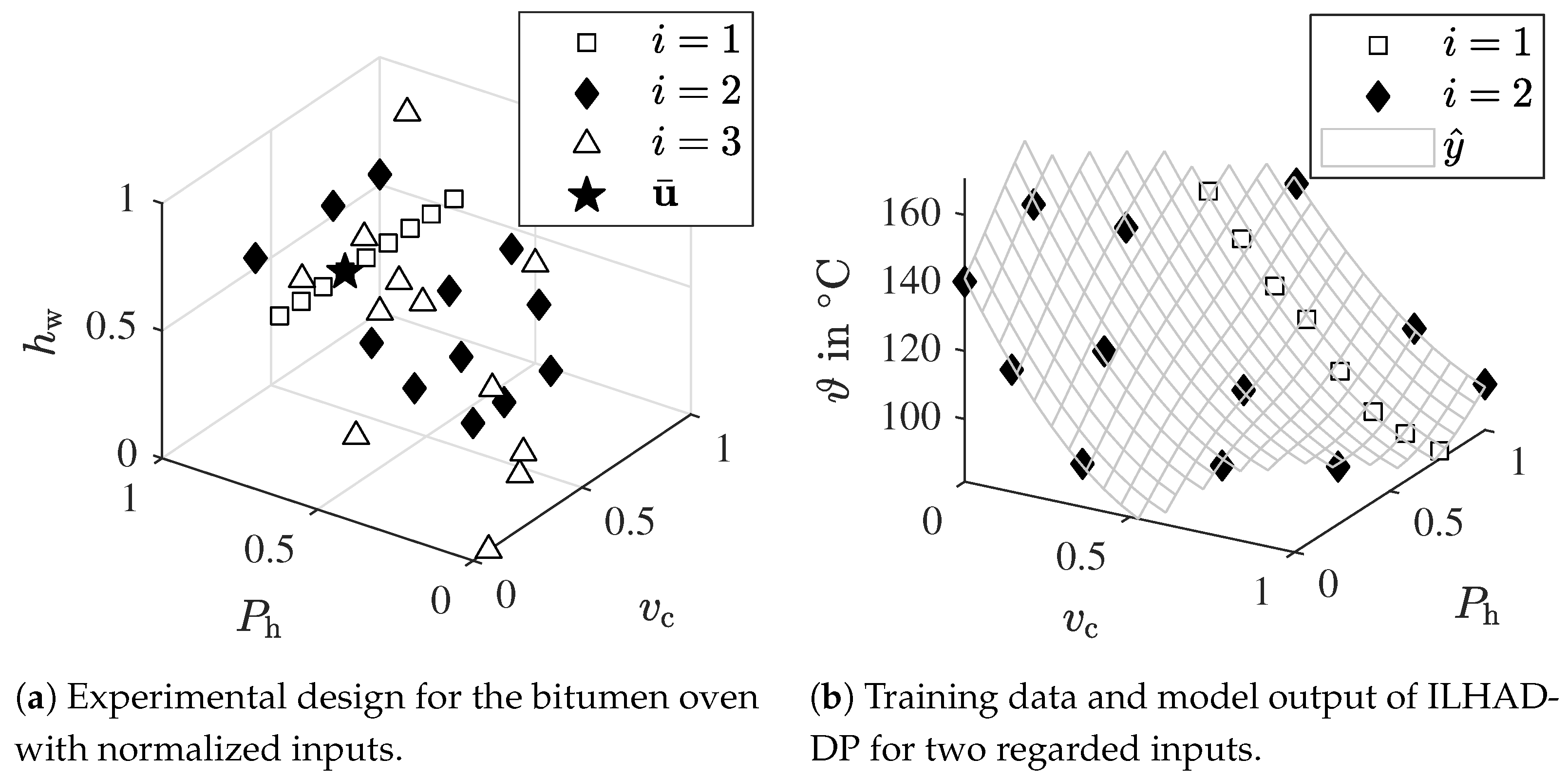
Real industrial processes typically possess inputs that differ in the type of functional relationship and the impact onto the process output. Therefore, a more realistic test function is regarded as follows:

$$\begin{array}{cc}\hfill y(k)=& 4{({\tilde{u}}_1(k)-2+8{\tilde{u}}_2(k)-8{\tilde{u}}_2^2(k))}^2+{(3-4{\tilde{u}}_2(k))}^2+16\sqrt{{\tilde{u}}_3(k)+1}{(2{\tilde{u}}_3(k)-1)}^2\hfill \\ \hfill & +\sum _{m=4}^{8}mln\left(1+\sum _{n=3}^m{\tilde{u}}_n(k)\right)\hfill \end{array}$$

(16)

which is used in [46] to compare non-uniform LHC designs. It consists of eight inputs ${\tilde{u}}_j$, with $j=1,\dots ,8$ that differ in the nonlinearity of the main effect and in the strength of the interactions. The ranking of the inputs is obtained by varying each input over the entire range ${\tilde{u}}_j\in [0,1]$, with all other inputs fixed at the value ${\tilde{u}}_m=0.5\forall m\ne j$. The input that causes the largest range of output values is considered the most important one. In this way, the mapping of the input vector onto the inputs of the test function $\mathbf{u}\to [{\tilde{u}}_7,{\tilde{u}}_2,{\tilde{u}}_1,{\tilde{u}}_3,{\tilde{u}}_4,{\tilde{u}}_5,{\tilde{u}}_6,{\tilde{u}}_8]$ is derived.

Table 4. Comparison of the ILHAD-DP, ILHAD-NS and a single-step model for different numbers of steps and noise levels. All results are presented for test function (16), an operating point $\overline{\mathbf{u}}=[0.5\dots 0.5]$ and $N=[2120\dots 20]$ training data points. The RMSE is evaluated on $p^{*}$-dimensional test data with ${\sigma }_{\mathrm{t}}=0.36$. Mean values and standard deviations over 40 repetitions per parameter set are given, with the best mean values in bold print.

Maximal	Noise	ILHAD-DP	ILHAD-NS	Single Step
Step	Level	Model:	Model:	GPR Model:
${\mathit{p}}^{*}$	${\mathit{\sigma }}_{\mathbf{n}}$	$\mathbf{RMSE}$	$\mathbf{RMSE}$	$\mathbf{RMSE}$
4	${10}^{-3}$	$\mathbf{0}.\mathbf{0019}\pm \mathbf{0}.\mathbf{0005}$	$0.0038\pm 0.0040$	$0.0135\pm 0.0002$
	${10}^{-2}$	$\mathbf{0}.\mathbf{0128}\pm \mathbf{0}.\mathbf{0042}$	$0.0154\pm 0.0119$	$0.0142\pm 0.0006$
6	${10}^{-3}$	$\mathbf{0}.\mathbf{0046}\pm \mathbf{0}.\mathbf{0035}$	$0.0201\pm 0.0240$	$0.0131\pm 0.0003$
	${10}^{-2}$	$0.0193\pm 0.0112$	$0.1143\pm 0.4884$	$\mathbf{0}.\mathbf{0126}\pm \mathbf{0}.\mathbf{0025}$
8	${10}^{-3}$	$0.0155\pm 0.0072$	$0.0923\pm 0.0018$	$\mathbf{0}.\mathbf{0016}\pm \mathbf{0}.\mathbf{0001}$
	${10}^{-2}$	$0.0280\pm 0.0110$	$0.1777\pm 0.0086$	$\mathbf{0}.\mathbf{0063}\pm \mathbf{0}.\mathbf{0006}$

presents the model quality of both types of ILHAD models with different numbers of performed steps and noise levels. Both ILHAD models are compared to a single-step model, for which the test data distribution (11) with ${\sigma }_{\mathrm{t}}=0.36$ is used. In this way, the model quality is evaluated with a slight focus on the operating point.

For the smallest number of performed modeling steps $p^{*}=4$ and the low noise level ${\sigma }_{\mathrm{n}}={10}^{-3}$, both ILHAD models achieve a higher model quality than the single-step model, with the best results given for ILHAD-DP. With increasing noise (${\sigma }_{\mathrm{n}}={10}^{-2}$), a stronger increase in error of the ILHAD models is visible, compared to the single-step model. This indicates that both ILHAD models are more sensitive to noise than the single-step model. A higher noise level also reduces the stability of the incremental model construction, which is indicated by larger standard deviations of the RMSE.

With more modeling steps $p^{*}$ performed, an increasing RMSE of the incremental models for each noise level is visible. This behavior is caused by the incremental model structure in which errors of the submodels may sum up. For the single-step model, the RMSE decreases with the increasing dimensionality of the input space. This decrease is caused by the additional points in the global optimal LHC design and the applied ranking of the inputs. This ranking causes the additional inputs to be of minor importance for the overall model quality such that the complexity of the modeling task is not significantly increased. Furthermore, in each step, the number of design points in the LHC of the single-step model is increased by 20, contributing to a better estimation of all effects. In this way, the single-step model achieves the best results for a higher number of modeling steps. All in all, the results indicate that ILHAD models are well suited for a low number of inputs and a low noise level. In this experiment, ILHAD-DP provides a better model quality than ILHAD-NS. ILHAD-NS suffers from a more unstable model construction, leading to much worse results in single runs. As an example, for $p^{*}=6$ and ${\sigma }_{\mathrm{n}}={10}^{-2}$, the error and the standard deviation are dominated by a single run with a RMSE value of $3.42$.

4.2. Bitumen Oven

As a real-world use case, the ILHAD method is applied to a bitumen oven of Miele & Cie. KG, which is used for melting sheets of bitumen on water containers of washing machines. Unprocessed parts with sheets of bitumen on top can be seen in Figure 9 at the entry of the oven.

A conveyor belt is used to continuously move the parts through the oven in which the sheets of bitumen are heated up by infrared heaters. At the end of the oven, a contact-free measurement of the resulting surface temperature $\vartheta$ of each part is made. In order to achieve a reliable bonding of the bitumen, a sufficient temperature must be reached. This temperature should be predicted by a process model to enable an optimization of the process parameters. In this way, a high bonding quality for different types of parts with minimal power consumption should be achieved.

The main inputs of the process are the conveyor speed $v_{\mathrm{c}}$, which can be varied continuously, and the heating power $P_{\mathrm{h}}$ for which five discrete values can be selected. In addition, the height of the water containers $h_{\mathrm{w}}$ has a slight influence on the surface temperature, due to the directional characteristic of the infrared heaters. Five different types of water containers with specific heights are regarded. A ranking of the inputs based on domain knowledge leads to the input vector $\mathbf{u}=[v_{\mathrm{c}}{P}_{\mathrm{h}}{h}_{\mathrm{w}}]$. As the first input, the conveyor speed is preferred over the heating power because it can be varied more easily. A variation of the heating power requires additional heat-up time of the infrared heater, which would increase the measurement time in the first ILHAD step.

The resulting experimental design for step $p^{*}=3$ with $N=[9,12,12]$ design points is depicted in Figure 10a.

To prevent insufficient and excessive surface temperatures of the bitumen, constraints in the input space are defined based on domain knowledge and data from the first ILHAD step. In this way, areas in the input space with low conveyor speed and high heating power or high conveyor speed and low heating power are avoided. The inputs $P_{\mathrm{h}}$ and $h_{\mathrm{w}}$ can only be varied in steps, which define the possible LHC levels. In addition to the level of the operating point, both inputs only possess four levels, which would limit the number of possible design points to four in step $i=2$ and $i=3$. To enable the acquisition of sufficient data points, each level is occupied by three design points so that no LHC is given anymore. However, a space-filling design is still created by applying the EDLS algorithm, which is extended to incorporate the defined constraints in the input space.

The training data points in steps $i=1$ and $i=2$ and the exemplary model output of ILHAD-DP in the second step $\widehat{y}$, depicted as a grid, are presented in Figure 10b. To evaluate the estimated models, an additional 15 test data points are measured, which are defined by an optimized LHC in the constrained input space.

Table 5. Comparison of incremental model structures for the bitumen oven. The RMSE on the additional test data points is presented in different ILHAD steps.

Step	Polynomial	Local Model	ILHAD-DP	ILHAD-NS
	Model:	Tree:	Model:	Model:
	RMSE in °C	RMSE in °C	RMSE in °C	RMSE in °C
1	27.62	29.69	26.44	26.44
2	6.37	4.63	4.83	4.81
3	4.32	4.07	3.02	3.29

compares the prediction accuracy of different incremental models based on these test data points.

As more inputs and functional relationships are incorporated into the incremental models, the gain in accuracy in every ILHAD step can be seen. All models provide a similar model quality, with ILHAD-DP achieving the best results in the last step $p^{*}=3$. The RMSE value of approximately $3{}^{\circ }\mathrm{C}$ indicates a sufficient model quality for practical application, as a temperature interval of $10{}^{\circ }\mathrm{C}$ is specified as the target value of the bitumen temperature.

5. Discussion

In the following, the obtained results are discussed. As the proposed methodology not only focuses on the model quality, additional aspects concerning the role of the domain expert and the applicability for industrial processes are discussed as well.

5.1. Model Quality

Making use of GPR models as the submodel structure increases the flexibility of the incremental model and leads to a higher overall model quality in the incremental model structure, compared to local linear model trees and polynomial models. Due to its construction mechanism, an incremental model is focused on an operating point in which high model quality is achieved, whereas the single step models are trained on a more uniform training data distribution, leading in general to lower RMSE values in the whole input space (see Table 1). Compared to the single-step models, ILHAD causes a higher variation in the RMSE, especially for test data covering the whole input space. This can be explained by the smaller number of data points in each step, leading to larger gaps in the input space of each submodel. Due to the random initialization of the LHC, the position of the gaps varies. In some runs, these gaps are located in areas with a strongly nonlinear process behavior, leading to a high variation in the obtained RMSE. However, many real industrial processes can be expected to be less nonlinear than the used test function (13), leading to a reduction of this effect.

For different types of functional relationships, ILHAD models achieve a higher model quality close to the operating point, compared to the single-step models (see Table 2). The best case scenario for ILHAD is given with test function (14), in which independent functional relationships for each input are present. Each design ${\mathcal{D}}_i$ used for estimating the incremental model is a LHC, which is a non-collapsing design. This means that a projection of a LHC in a lower-dimensional subspace is still a space-filling design, which is beneficial if the inputs are irrelevant [34]. In this particular case with no interactions between the inputs, each model $f_i$ only models the influence of input $u_i$, whereas all the other inputs are irrelevant. This means that for estimating $f_i$, the LHC collapses to equally spaced points in $u_i$, which is a well-suited point distribution for GPR model estimation. The worst case scenario for ILHAD is given with test function (15), because neither the ranking of the inputs nor the projection capabilities of the LHC can be exploited. Nevertheless, the incremental model is able to model the interactions between the inputs and provides a good model quality, especially close to the operating point.

As the experiments presented in Table 4 indicate, ILHAD models are more sensitive to noise than the single-step GPR models. Due to the smaller number of data points in each step, each submodel of ILHAD is more affected by random fluctuations in the data, whereas the single step models are trained on a higher number of data points so that random fluctuations are more likely to be compensated. In addition, with an increasing number of modeling steps, the benefit in model quality of the incremental model structure fades. If a new submodel is added, the incremental model structure ensures that the overall process model is not changed in the previously regarded subspace. However, this property also prevents additional submodels from correcting the error of previous ones in this subspace. Nevertheless, no suitable correction of the previous model is expected because more complex functional relationships need to be modeled by the additional submodels in a higher dimensional input space, with only a few data points given. These more complex functional relationships result from interactions, which can be expected to occur more likely if a higher number of inputs is given.

As no correction of an already created submodel is possible, submodels with a high generalization capability and the ability to represent all significant interactions are needed. Making use of a sequential design strategy within each step of ILHAD is a further research direction to improve the model quality and the stability of the incremental model. Starting from an initial space-filling design with a low number of data points in each step, additional design points can be added successively. Some strategies for creating such sequential space-filling designs are discussed in [23]. This method can make use of the interpretable length scales in ILHAD-DP and ILHAD-NS. The more interactions between the inputs are detected, the more data points should be added to the design. Moreover, an extension of this approach toward active learning is possible. In active learning, a sequential design is created with an optimization criterion based on the current model. In this way, new data points are placed such that the best improvement of the model can be expected. Active learning strategies for GPR models are, for example, based on the output variance and were successfully applied to industrial processes [47].

Regarding the model quality, it can be concluded that ILHAD is well suited for industrial processes with few inputs and low output noise. However, reaching a higher model quality than the single-step model is not the main aim of the proposed methodology. Due to the less uniform point distribution of ILHAD in the input space, a higher model error can be expected in general if significant interactions between the inputs are present. Nevertheless, the methodology possesses several advantages over classical DoE and modeling approaches in terms of interpretability and applicability for industrial processes, which are discussed in the following.

5.2. The Role of Domain Experts

Domain knowledge plays an important role in the ILHAD methodology. A domain expert defines the operating point, used as the starting point for the exploration of the process behavior. In ILHAD, a high model quality around this operating point can be expected. Even though the whole input space is explored and modeled by ILHAD, the choice of this point also has an influence on the overall model quality as indicated by Table 1. This can be explained by interactions between the inputs that affect the functional relationships present in the data. These functional relationships are more or less complex, dependent on the values of further inputs that are defined by the operating point. The choice of the operating point, therefore, depends on the purpose of the model. If a high overall model quality is required, an operating point should be used in which preferably no functional relationships are suppressed due to interactions. Another important task that can be performed based on expert knowledge is the ranking of the inputs. This ranking affects the number of ILHAD steps needed to achieve a desired overall model quality. If a suitable ranking is chosen, the ILHAD methodology might be terminated after a few steps, leading to a low measurement effort. To support a domain expert in determining this input ranking, automatic methods based on data from normal process operation can additionally be used. For example, methods that evaluate the correlation between the inputs and outputs may be suitable [48]. Finally, for real industrial processes, the definition of the feasible input space is crucial for performing safe and successful measurements. For typical experimental designs, this is a complex task due to the high dimensionality of the input space and the simultaneous variation of all inputs. Due to the lower dimensionality in the first ILHAD steps, this task is simplified.

As the success of the measurements and the achievable model quality depend on domain knowledge, the domain expert that provides this knowledge must be supported. ILHAD possesses several characteristics that simplify the incorporation of domain knowledge and the verification of the model. As measurement and modeling in ILHAD start with a one-dimensional input space, the complexity is low and increases in each step. Similar to the one-factor-at-a-time method [49], this is a more intuitive procedure for most humans than classical experimental designs. In particular, the first steps are easy to understand and visualize, creating confidence toward the model. As in each step of ILHAD, a usable process model is created, this model can be used to simplify the determination of the feasible input space in the next step. Based on the current model, critical areas in the input space can be identified in which the effect of only one additional input must be evaluated. As an example, a current ILHAD model predicts a temperature close to a specified temperature limit in an area of the input space. The domain expert only needs to assess the effect of the newly added input and if it will lead to an increase in temperature, violating the temperature limit. Compared to the single-step GPR model with ARD, it is not only possible to detect irrelevant inputs, but the length scales of the submodels also indicate interactions between the inputs. This enables insights into the process behavior and can be used to validate the model based on expert knowledge.

5.3. Comparison of ILHAD-DP and ILHAD-NS

Both presented methods for zero-forcing in a subspace provide similar results for a small number of modeling steps and low noise. ILHAD-DP requires no changes to the kernel function and enables using all information provided by the GPR model, such as the confidence interval of the model output. However, due to the diagonal offset in the kernel matrix and spaces in between the dummy points, a slight nonzero output for each submodel might occur (see Figure 7b). This non-zero model output does not significantly degrade the model as indicated by a similar RMSE close to the operating point, such as ILHAD-NS, which realizes an exact submodel output of zero. Due to the dummy points, ILHAD-DP causes a higher computational effort than ILHAD-NS. The dummy points increase the model complexity and the number of parameters. In addition, the creation of the space-filling design with the EDLS algorithm for populating the subspace with dummy points is computationally demanding, especially for high dimensionality of this subspace. However, due to the relatively small sample size in DoE for industrial processes and only the few modeling steps that are performed, this additional computational effort of ILHAD-DP has low relevance in practice.

With strong interactions present, ILHAD-NS achieves better results than ILHAD-DP (see test function (15) in Table 2). This can be explained by the zero-forcing property, which has a stronger influence on the submodel if interactions are present. In ILHAD-NS, this zero-forcing property is incorporated into the hyperparameter optimization loop, leading to a better submodel fit. In ILHAD-DP, hyperparameter optimization is performed without the dummy points so that the changes introduced by the zero-forcing property are not taken into account. Furthermore, the higher variation of the RMSE in most experiments indicates that ILHAD-NS is less stable than ILHAD-DP. Especially for higher noise levels and a higher number of modeling steps, the RMSE increases. This can be explained by the modification of the kernel function, leading to distortions close to the previously regarded subspace. Another drawback of this modification is that the confidence interval of the model output is not valid anymore.

5.4. Applicability

The creation of classical experimental designs requires a prior specification of all inputs that should be regarded in the experiment. In practice, this may lead to a higher dimensionality of the experimental design and the input space of the model than necessary. If the relevance of an input is questionable according to the current level of knowledge, it is more reasonable to incorporate it into the design, because otherwise, the resulting process model might perform badly, due to the missing information. ILHAD can reduce the measurement effort, because the number of inputs does not need to be predefined. After each step, the suitability of the model for practical usage can be evaluated and further inputs can be added, if required. This keeps the dimensionality of the input space low, leading to a less complex and better interpretable model.

In the presented real-world experiment, additional benefits of ILHAD in terms of applicability become apparent. ILHAD offers a simplified measurement procedure for real industrial plants, due to the increasing complexity in each step. As only a few inputs are varied in the first steps, supervision of the process behavior is simplified. In particular, there is no need to simultaneously vary all process inputs at the beginning of the measurements, which might cause unexpected process behavior, or even defects of the plant, due to infeasible design points. Furthermore, information from the previous ILHAD steps can be used to assess the feasibility of design points in the next steps. At the bitumen oven, critical values of the conveyor speed, determined in the first step, are used to better define infeasible regions in the input space for the next steps. Due to the fixing of later considered process inputs to the level of the operating point, fewer variations of these inputs are required. If the variation of an input value is a manual task or takes some time, ILHAD can reduce the actuation effort or the measurement time. In the use case of the bitumen oven, a variation of the heating power is time consuming because a heat-up time of approximately five minutes is required after every change. As the heating power is constant in the first ILHAD step, the measurement time is reduced compared to a LHC design in which a new value of the heating power is selected for every point.

6. Conclusions

This paper presented the incremental Latin hypercube additive design (ILHAD) methodology with Gaussian process regression models (GPR) as a submodel structure, which is an applicable method for modeling industrial processes. In ILHAD, alternating DoE and modeling steps with an increasing number of regarded inputs are performed so that a process model is incrementally extended by new additive submodels. In order to prevent a degradation of the overall process model, each submodel ensures, due to its structure, that the previous model remains unchanged in its region of validity. To realize this behavior for GPR submodels, two different approaches—ILHAD-DP and ILHAD-NS—were presented. In ILHAD, measurement procedures and models are established, which are simple in the first step and become more complex as the number of steps increases. This procedure with increasing complexity represents a more intuitive approach than classical DoE procedures.

The model quality of the incremental models was investigated in comparison to a model estimated in a single step on the basis of a classical space-filling design. The proposed incremental models are able to achieve a high model quality in an area around the specified operating point, which is typically most relevant for practical usage of a process model in industry. Process characteristics that favor a high model quality of ILHAD were identified on the basis of computer simulation experiments. Beneficial characteristics are mainly additive functional relationships between the inputs and the output and a low noise level at the process output. In this way, even a higher model quality in the whole input space, compared to the single-step model, can be achieved. The experimental design and the resulting model can be adapted to the specific needs of the regarded use case by incorporating domain knowledge. Such knowledge is used for selecting an operating point, defining the feasible input space and determining a suitable input ranking. If proper domain knowledge is provided, a high model quality can be reached where it is required, safe experiments can be performed, and the number of measurements steps might be reduced. Moreover, characteristics of ILHAD that support the incorporation of domain knowledge and the validation of the model were presented. These include the usage of previous models for evaluating the feasibility of design points and the interpretability of the kernel length scales of each submodel, enabling the detection of different types of effects. Furthermore, the applicability of this methodology for modeling real industrial processes was demonstrated by the example of a bitumen oven.

In most experiments, the ILHAD-DP method reached a higher model quality than ILHAD-NS. The main issue in both methods is an unstable model construction, caused by an insufficient number of data points, if strong interactions between the inputs are present. Making use of a sequential design strategy in each ILHAD step, which can further be extended toward an active learning approach, is proposed as a new research direction.

References

1. Hirsch-Kreinsen, H.; Kubach, U.; von Wichert, G.; Hornung, S.; Hubrecht, L.; Sedlmeir, J.; Steglich, S. Key Themes of Industrie 4.0; Technical Report; Research Council of the Plattform Industrie 4.0: Munich, Germany, 2019. [Google Scholar]
2. Fisher, O.J.; Watson, N.J.; Escrig, J.E.; Witt, R.; Porcu, L.; Bacon, D.; Rigley, M.; Gomes, R.L. Considerations, challenges and opportunities when developing data-driven models for process manufacturing systems. Comput. Chem. Eng. 2020, 140, 106881. [Google Scholar] [CrossRef]
3. Freiesleben, J.; Keim, J.; Grutsch, M. Machine learning and Design of Experiments: Alternative approaches or complementary methodologies for quality improvement? Qual. Reliab. Eng. Int. 2020, 36, 1837–1848. [Google Scholar] [CrossRef]
4. Freeman, L.J.; Ryan, A.G.; Kensler, J.L.K.; Dickinson, R.M.; Vining, G.G. A Tutorial on the Planning of Experiments. Qual. Eng. 2013, 25, 315–332. [Google Scholar] [CrossRef]
5. Simpson, J.R.; Listak, C.M.; Hutto, G.T. Guidelines for Planning and Evidence for Assessing a Well-Designed Experiment. Qual. Eng. 2013, 25, 333–355. [Google Scholar] [CrossRef]
6. Voigt, T.; Kohlhase, M.; Nelles, O. Incremental Latin Hypercube Additive Design for LOLIMOT. In Proceedings of the 25th IEEE International Conference on Emerging Technologies and Factory Automation (ETFA 2020), Vienna, Austria, 8–11 September 2020; pp. 1602–1609. [Google Scholar]
7. Nelles, O. Nonlinear System Identification: From Classical Approaches to Neural Networks, Fuzzy Models, and Gaussian Processes; Springer Nature: Berlin/Heidelberg, Germany, 2020. [Google Scholar]
8. Schielzeth, H. Simple means to improve the interpretability of regression coefficients. Methods Ecol. Evol. 2010, 1, 103–113. [Google Scholar] [CrossRef]
9. Hastie, T.J.; Tibshirani, R.J. Generalized Additive Models; Chapman and Hall/CRC: Boca Raton, FL, USA, 1990. [Google Scholar]
10. Bujalski, M.; Madejski, P. Forecasting of Heat Production in Combined Heat and Power Plants Using Generalized Additive Models. Energies 2021, 14, 2331. [Google Scholar] [CrossRef]
11. Duvenaud, D.; Nickisch, H.; Rasmussen, C.E. Additive Gaussian Processes. In Proceedings of the 24th International Conference on Neural Information Processing Systems, Granada, Spain, 12–15 December 2011; Curran Associates Inc.: Red Hook, NY, USA, 2011; NIPS’11, pp. 226–234. [Google Scholar]
12. Yeom, C.U.; Kwak, K.C. The Development of Improved Incremental Models Using Local Granular Networks with Error Compensation. Symmetry 2017, 9, 266. [Google Scholar] [CrossRef] [Green Version]
13. Pedrycz, W.; Kwak, K.C. The development of incremental models. IEEE Trans. Fuzzy Syst. 2007, 15, 507–518. [Google Scholar] [CrossRef]
14. Friedman, J.H. Stochastic gradient boosting. Comput. Stat. Data Anal. 2002, 38, 367–378. [Google Scholar] [CrossRef]
15. Chen, T.; Guestrin, C. XGBoost: A Scalable Tree Boosting System. In Proceedings of the 22nd ACM SIGKDD International Conference on Knowledge Discovery and Data Mining, San Francisco, CA, USA, 13–17 August 2016; Association for Computing Machinery: New York, NY, USA, 2016; KDD ’16, pp. 785–794. [Google Scholar] [CrossRef] [Green Version]
16. Montgomery, D. Design and Analysis of Experiments; John Wiley & Sons, Inc.: Hoboken, NJ, USA, 2017. [Google Scholar]
17. Astakhov, V.P. Screening (sieve) design of experiments in metal cutting. In Design of Experiments in Production Engineering; Springer: Cham, Switzerland, 2016; pp. 1–37. [Google Scholar]
18. Santner, T.J.; Williams, B.J.; Notz, W.I. The Design and Analysis of Computer Experiments; Springer: New York, NY, USA, 2018. [Google Scholar] [CrossRef]
19. Chen, C.C.; Chiang, K.T.; Chou, C.C.; Liao, Y.C. The use of D-optimal design for modeling and analyzing the vibration and surface roughness in the precision turning with a diamond cutting tool. Int. J. Adv. Manuf. Technol. 2011, 54, 465–478. [Google Scholar] [CrossRef]
20. Emmert-Streib, F.; Dehmer, M. Evaluation of Regression Models: Model Assessment, Model Selection and Generalization Error. Mach. Learn. Knowl. Extr. 2019, 1, 521–551. [Google Scholar] [CrossRef] [Green Version]
21. Saleh, A.K.M.E.; Arashi, M.; Kibria, B.M.G. Theory of Ridge Regression Estimation with Applications; John Wiley & Sons: Hoboken, NJ, USA, 2019; Volume 285. [Google Scholar]
22. Rasmussen, C. Gaussian Processes for Machine Learning; MIT Press: Cambridge, MA, USA, 2006. [Google Scholar]
23. Lu, L.; Anderson-Cook, C.M.; Martin, M.; Ahmed, T. Practical choices for space-filling designs. Qual. Reliab. Eng. Int. 2021. [Google Scholar] [CrossRef]
24. Kleijnen, J.P.C. Design and Analysis of Simulation Experiments; Springer: Cham, Switzerland, 2015. [Google Scholar]
25. Cabral-Farias, R.; Pronzato, L.; Rendas, M.J. Incremental construction of nested designs based on two-level fractional factorial designs. Preprint hal-02483004. 2020. Available online: https://hal.archives-ouvertes.fr/hal-02483004 (accessed on 29 August 2021).
26. Lu, L.; Anderson-Cook, C.M. Strategies for sequential design of experiments and augmentation. Qual. Reliab. Eng. Int. 2020. [Google Scholar] [CrossRef]
27. Tharwat, A.; Schenck, W. Balancing Exploration and Exploitation: A novel active learner for imbalanced data. Knowl.-Based Syst. 2020, 210, 106500. [Google Scholar] [CrossRef]
28. Sheng, X.; Ma, J.; Xiong, W. Smart Soft Sensor Design with Hierarchical Sampling Strategy of Ensemble Gaussian Process Regression for Fermentation Processes. Sensors 2020, 20, 1957. [Google Scholar] [CrossRef] [PubMed] [Green Version]
29. Wu, J.; Luo, Z.; Zheng, J.; Jiang, C. Incremental modeling of a new high-order polynomial surrogate model. Appl. Math. Model. 2016, 40, 4681–4699. [Google Scholar] [CrossRef]
30. Schrangl, P.; Tkachenko, P.; del Re, L. Iterative Model Identification of Nonlinear Systems of Unknown Structure: Systematic Data-Based Modeling Utilizing Design of Experiments. IEEE Control Syst. Mag. 2020, 40, 26–48. [Google Scholar] [CrossRef]
31. Fang, K.T.; Li, R.; Sudjianto, A. Design and Modeling for Computer Experiments; Chapman and Hall/CRC: New York, NY, USA, 2005. [Google Scholar]
32. Ji, Y.B.; Alaerts, G.; Xu, C.J.; Hu, Y.Z.; Heyden, Y.V. Sequential uniform designs for fingerprints development of Ginkgo biloba extracts by capillary electrophoresis. J. Chromatogr. A 2006, 1128, 273–281. [Google Scholar] [CrossRef] [PubMed]
33. Winker, P.; Fang, K.T. Optimal U—Type Designs. In Monte Carlo and Quasi-Monte Carlo Methods 1996; Springer: New York, NY, USA, 1998; pp. 436–448. [Google Scholar] [CrossRef]
34. Pronzato, L.; Müller, W.G. Design of computer experiments: Space filling and beyond. Stat. Comput. 2012, 22, 681–701. [Google Scholar] [CrossRef]
35. Guan, S.U.; Liu, J. Incremental Neural Network Training with an Increasing Input Dimension. J. Intell. Syst. 2004, 13, 43–70. [Google Scholar] [CrossRef]
36. Bellman, R.E. Adaptive Control Processes; Princeton University Press: Princeton, NJ, USA, 1961. [Google Scholar] [CrossRef]
37. Viana, F.A.C. Things you wanted to know about the Latin hypercube design and were afraid to ask. In Proceedings of the 10th World Congress on Structural and Multidisciplinary Optimization, Orlando, FL, USA, 19–24 May 2013; Volume 19. [Google Scholar]
38. Ebert, T.; Fischer, T.; Belz, J.; Heinz, T.O.; Kampmann, G.; Nelles, O. Extended Deterministic Local Search Algorithm for Maximin Latin Hypercube Designs. In Proceedings of the IEEE Symposium Series on Computational Intelligence, Cape Town, South Africa, 7–10 December 2015. [Google Scholar]
39. Chen, S.; Montgomery, J.; Bolufé-Röhler, A. Measuring the curse of dimensionality and its effects on particle swarm optimization and differential evolution. Appl. Intell. 2014, 42, 514–526. [Google Scholar] [CrossRef]
40. Bergmann, D.; Harder, K.; Niemeyer, J.; Graichen, K. Nonlinear MPC of a Heavy-Duty Diesel Engine with Learning Gaussian Process Regression. IEEE Trans. Control. Syst. Technol. 2021, 1–17. [Google Scholar] [CrossRef]
41. Goldberg, P.W.; Williams, C.K.I.; Bishop, C.M. Regression with input-dependent noise: A Gaussian process treatment. Adv. Neural Inf. Process. Syst. 1997, 10, 493–499. [Google Scholar]
42. Genton, M.G. Classes of kernels for machine learning: A statistics perspective. J. Mach. Learn. Res. 2001, 2, 299–312. [Google Scholar]
43. Lowe, D. Radial basis function networks-revisited. Math. Today 2015, 51, 124–126. [Google Scholar]
44. Sobol, I.M. On the distribution of points in a cube and the approximate evaluation of integrals. USSR Comput. Math. Math. Phys. 1967, 7, 86–112. [Google Scholar] [CrossRef]
45. Friedman, J.H. Multivariate adaptive regression splines. Ann. Stat. 1991, 19, 1–67. [Google Scholar] [CrossRef]
46. Dette, H.; Pepelyshev, A. Generalized Latin Hypercube Design for Computer Experiments. Technometrics 2010, 52, 421–429. [Google Scholar] [CrossRef] [Green Version]
47. Yue, X.; Wen, Y.; Hunt, J.H.; Shi, J. Active Learning for Gaussian Process Considering Uncertainties with Application to Shape Control of Composite Fuselage. IEEE Trans. Autom. Sci. Eng. 2021, 18, 36–46. [Google Scholar] [CrossRef]
48. Guyon, I.; Elisseeff, A. An introduction to variable and feature selection. J. Mach. Learn. Res. 2003, 3, 1157–1182. [Google Scholar]
49. Czitrom, V. One-Factor-at-a-Time versus Designed Experiments. Am. Stat. 1999, 53, 126–131. [Google Scholar]
Figure 1. Schematic two-dimensional input space of an industrial process. Without performing experiments, data can only be gathered from the operational area.
Mathematics 09 02479 g001
Figure 2. Trade-off between information content and measurement effort, with qualitative grading of different methods for data acquisition.
Mathematics 09 02479 g002
Figure 3. Flowchart of the ILHAD methodology.
Mathematics 09 02479 g003
Figure 4. Structure of the incremental process model. In each of the p * steps, a new submodel is added to the structure. For simplicity, only the first three submodels are shown.
Mathematics 09 02479 g004
Figure 5. Estimation of the i-th submodel, modeling the difference y ˜ i between the process output y and the summed up outputs of all existing models y Σ . The composition of the process input vector u is depicted, whereas the models only use the inputs u i specified by the experimental design.
Mathematics 09 02479 g005
Figure 6. Overall experimental designs in the (a) second and (b) third step with N = [ 11 16 20 ] data points and the operating point u ¯ = [ 0.5 0.5 0.5 ] .
Mathematics 09 02479 g006
Figure 7. A 2D example for illustrating the mechanism for zero-forcing in ILHAD-DP. The model is trained on its specific training data points and additional dummy points. The dummy points lead to a model output of approximately zero in the previously regarded subspace.
Mathematics 09 02479 g007
Figure 8. RMSE of ILHAD-DP and the single step GPR model for different standard deviations σ t of the test data. Average values over 40 repetitions are given for p * = 3 modeling steps, a noise level of σ n = 10 3 , an operating point u ¯ = [ 0.7 0.7 0.7 ] and N = [ 11 16 20 ] training data points.
Mathematics 09 02479 g008
Figure 9. The entry of the bitumen oven of Miele & Cie. KG is shown. Several water containers with sheets of bitumen on top are visible.
Mathematics 09 02479 g009
Figure 10. Experimental design for all p * = 3 ILHAD steps performed at the bitumen oven and the resulting model output of ILHAD-DP in step i = 2 .
Mathematics 09 02479 g010