Analysis of a Novel Two-Dimensional Lattice Hydrodynamic Model Considering Predictive Effect

Abstract

In actual driving, the driver can estimate the traffic condition ahead at the next moment in terms of the current traffic information, which describes the driver’s predictive effect. Due to this factor, a novel two-dimensional lattice hydrodynamic model considering a driver’s predictive effect is proposed in this paper. The stability condition of the novel model is obtained by performing the linear stability analysis method, and the phase diagram between the driver’s sensitivity coefficient and traffic density is drawn. The nonlinear analysis of the model is conducted and the kink-antikink of modified Korteweg-de Vries (mKdV) equation is derived, which describes the propagation characteristics of the traffic density flow waves near the critical point. The numerical simulation is executed to explore how the driver’s predictive effect affects the traffic flow stability. Numerical results coincide well with theoretical analysis results, which indicates that the predictive effect of drivers can effectively avoid traffic congestion and the fraction of eastbound cars can also improve the stability of traffic flow to a certain extent.

1. Introduction

For the past few years, infrastructure construction of urban traffic networks has developed rapidly. However, with the rapid development of economy, the desire for convenient transportation of people is increasing, and the measures of road construction alone are insufficient for the growing needs of travel. Since traffic congestion is a common problem that needs to be solved urgently, several academics have committed considerable efforts to easing urban traffic congestion. Thereby, a large number of traffic flow models are proposed to explore the evolution law of traffic flow, such as car-following models [1,2,3,4,5,6,7,8,9], macro models [10,11,12,13,14,15], and lattice hydrodynamic models [16,17,18,19,20,21,22,23]. With the improvement of people’s living standard, as well as the rapid development of high-tech, some intelligent transportation models [24,25,26,27,28] have been proposed. The establishment and analysis of traffic flow model, whether for the development of traffic flow theory, or for the reality of traffic management, planning, and control, are greatly meaningful.

At present, most of scholars specializing in traffic flow theory have investigated the one-dimensional lattice hydrodynamic model, such as the self-stabilization effect [29,30], the flow difference effect [31], the density difference effect [32], and so on. There are both single-lane and two-lane models, so the investigation of one-dimensional lattice hydrodynamic model has been relatively mature. However, the actual urban road traffic is a network structure. Thereby, the exploration of a two-dimensional lattice hydrodynamic model is more significant and valuable. So far, there are still extremely few scholars who are involved in these fields. In 1999, Nagatani et al. [33] first extended the one-dimensional lattice hydrodynamic model to two dimensions without any reference, and performed analysis and numerical simulation. Redhu et al. [34] conducted a two-dimensional lattice hydrodynamic model to research the influence of the overtaking effect on the stability of traffic flow in two-dimensional traffic flow in a two-dimensional scene. Liu et al. [35] investigated the role of shared lane signs in two-dimensional actual traffic. Li et al. [36] executed a new feedback control signal to discuss, not only in detail but clearly, the effect of driver’s memory effect on two-dimensional actual traffic.

In actual driving, drivers tend to make predictions about the upcoming congestion based on the current traffic conditions. Therefore, it is crucial to thoroughly investigate the influence of prediction effect on the conditions of road traffic. At present, relevant studies have been carried out by scholars. Wang et al. [37] proposed a lattice hydrodynamic model of driver’s prediction effect in a single lane to explore traffic flow characteristics considering such driver’s behavior. Zhang et al. [38] also extended the driver’s prediction effect to the two-lane lattice model, and investigated the influence of this driver’s behavior on the two-lane road traffic. Kaur et al. [39] introduced the driver’s prediction effect into the single-lane lattice hydrodynamic model with overtaking effect. However, in the two-dimensional lattice hydrodynamic model, up to now, there has been no academics investigated on the influence of the prediction effect on the two-dimensional traffic flow. Therefore, in this paper, a novel two-dimensional lattice hydrodynamic considering prediction effect is put forward to fill this gap.

The remaining content of this paper is the following parts. The second part provides detailed information on the origin and development of the model. In the third part, the linear analysis is conducted and the deduced stability conditions were plotted as stability curves. In the fourth section, we perform the nonlinear analysis to derive the mKdV equation that is a nonlinear differential equations describing the evolution of density waves. Then, the novel model is simulated numerically and the results are compared with those of theoretical analysis. In the last section, the appropriate conclusions are given according to the previous theoretical analysis and numerical simulation results.

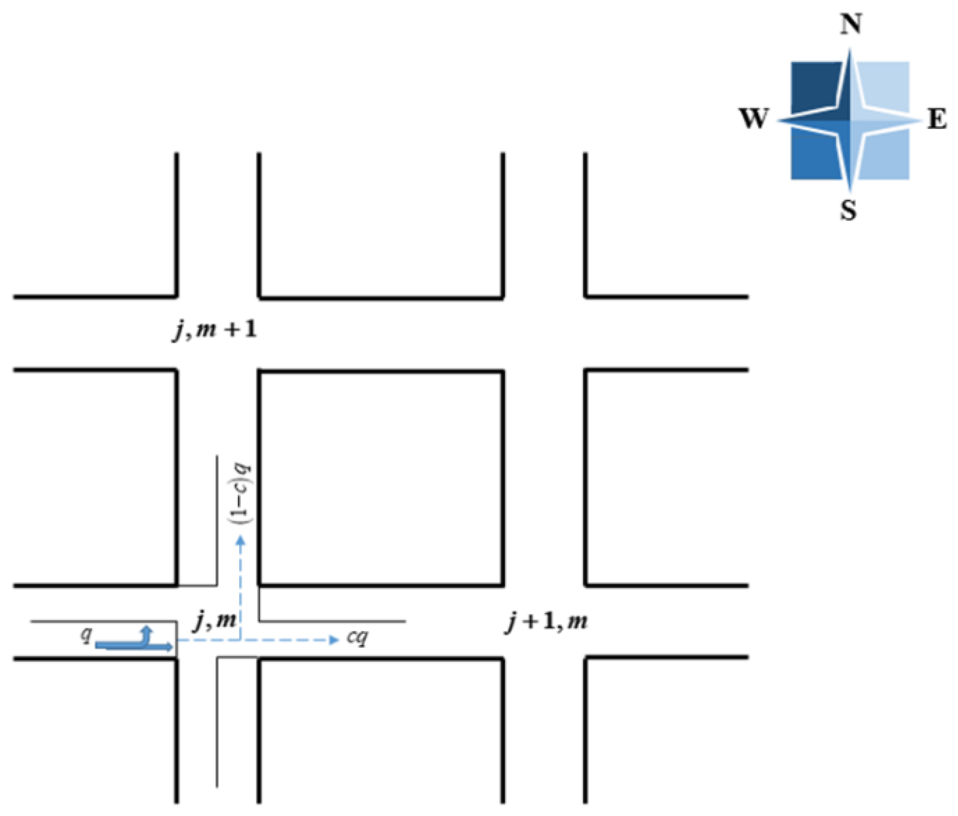
2. Methods: The Novel Two-Dimensional Lattice Model Considering Driver’s Predictive Effect

In 1998, a lattice hydrodynamic model for describing road traffic was first established by Nagatani et al. [16]. The optimal velocity function in the micro model is cleverly referenced by lattice model despite doing so as a macro model. Therefore, the model has the characteristics of both the macro model and the micro model. Furthermore, the model is comparatively easier to simulate due to discrete space variables and continuous time variables in this model. In order to make the model closer to the real road traffic, the two-dimensional lattice hydrodynamic model is extended from the one-dimensional model by Nagatani et al. [33].

The continuity equations of vehicles heading east and north are respectively given by Equations (1) and (2).

$${\partial }_t{\rho }_x\left(x,y,t\right) + {\partial }_x{\rho }_x\left(x,y,t\right)u\left(x,y,t\right) = 0,$$

(1)

$${\partial }_t{\rho }_y\left(x,y,t\right) + {\partial }_x{\rho }_y\left(x,y,t\right)v\left(x,y,t\right) = 0.$$

(2)

where ${\partial }_t = \partial /{\partial }_t$, ${\partial }_x = \partial /{\partial }_x$ and ${\partial }_y = \partial /{\partial }_y$. ${\rho }_x\left(x,y,t\right)$$\left[{\rho }_y\left(x,y,t\right)\right]$ and $u\left(x,y,t\right)$$\left[v\left(x,y,t\right)\right]$ indicate the density and speed of eastbound cars (northbound cars) on the two-dimensional lattice.

The continuity equations express the conservation of vehicles and reflect the relationship between the local density and the local average speed. In addition to the continuity equation, the model also contains the motion equation describing the traffic currents. Equations (3) and (4) are established on the condition that traffic flow is regulated by the optimal speed with a delay time. The motion equation of eastbound and northbound cars respectively are

$${\rho }_x\left(x,y,t+\tau \right)u\left(x,y,t+\tau \right) = c{\rho }_{0}V\left(\rho \left(x+x_0,y,t\right)\right),$$

(3)

$${\rho }_y\left(x,y,t+\tau \right)v\left(x,y,t+\tau \right) = \left(1-c\right){\rho }_{0}V\left(\rho \left(x,y+y_0,t\right)\right).$$

(4)

where $c$ and $1-c$ are the proportion of vehicles driving east and north, respectively. ${\rho }_0$ is on the behalf of the total average density as in the two-dimensional. $\rho \left(x,y,t\right)$ represents the local density and $\rho \left(x,y,t\right) = {\rho }_x\left(x,y,t\right) + {\rho }_y\left(x,y,t\right)$. $x_0$ and $y_0$ are respectively the average headway of eastbound cars and northbound cars. $\tau$ refers to the delay time mentioned above, which represents the time lag required for the traffic current to reach the optimal current after the change of traffic flow. When $c = 0$ or $1$, all vehicles will go straight or turn left. At this moment, thus, the two-dimensional model is transformed into a one-dimensional hydrodynamic traffic model.

As shown in Figure 1, we treat each crossroads as a grid. As we all know, some cars will continue to drive straight and others will take the left at the crossroads. $q$ represents traffic flow rate. If a certain intersection is the $j,m$ lattice, vehicles going straight through this intersection will enter the $j+1,m$ lattice, and turning left, will enter the $j,m+1$ lattice. The above equations are discretized differentially and the delay time $\tau$ is rewritten as the driver’s sensitivity $a$ where $a = 1/\tau$, the model equations of driving north and driving east are as follows:

$${\partial }_t{\rho }_{j,m}^x\left(t\right) + c{\rho }_0\left(q_{j,m}^x\left(t\right) - q_{j-1,m}^x\left(t\right)\right) = 0,$$

(5)

$${\partial }_t{\rho }_{j,m}^y\left(t\right) + \left(1-c\right){\rho }_0\left(q_{j,m}^y\left(t\right) - q_{j,m-1}^y\left(t\right)\right) = 0,$$

(6)

$${\partial }_t{q}_{j,m}^x\left(t\right) = ac{\rho }_{0}V\left({\rho }_{j+1,m}^x\left(t\right)\right) - a{q}_{j,m}^x\left(t\right),$$

(7)

$${\partial }_t{q}_{j,m}^y\left(t\right) = a\left(1-c\right){\rho }_{0}V\left({\rho }_{j,m}^y\left(t\right)\right) - a{q}_{j,m}^y\left(t\right).$$

(8)

With the development of traffic intelligence, drivers can acquire more information about vehicles around them, which is conducive for drivers to fully understand the current road traffic conditions and make accurate predictions. In order to investigate the consequence of driver predictive effect on the stability of two-dimensional traffic flow, we improved the above model. When the continuity equations (i.e., Equations (5) and (6)) remain unchanged, the equations of traffic currents (i.e., Equations (7) and (8)) to the north and east with the introduction of the prediction terms are respectively as follows:

$${\partial }_t{q}_{j,m}^x\left(t\right) = ac{\rho }_{0}V\left[{\rho }_{j+1,m}^x\left(t\right) + \beta \left({\rho }_{j+1,m}^x\left(t+\tau \right) - {\rho }_{j+1,m}^x\left(t\right)\right)\right] - a{q}_{j,m}^x\left(t\right),$$

(9)

$${\partial }_t{q}_{j,m}^y\left(t\right) = a\left(1-c\right){\rho }_{0}V\left[{\rho }_{j,m+1}^y\left(t\right) + \beta \left({\rho }_{j,m+1}^y\left(t+\tau \right) - {\rho }_{j,m+1}^y\left(t\right)\right)\right] - a{q}_{j,m}^y\left(t\right).$$

(10)

To simplify the expression, we perform the Taylor expansion for $\rho \left(t+\tau \right)$ with ignoring the nonlinear terms and then do the same for $V\left[\rho \left(t\right) + \beta \left(\rho \left(t+\tau \right) - \rho \left(t\right)\right)\right]$, which obtains the formula

$$V\left[\rho \left(t\right) + \beta \left(\rho \left(t+\tau \right) - \rho \left(t\right)\right)\right] = V\left(\rho \left(t\right)\right) + V^{\prime }\left(\rho \left(t\right)\right)\beta \tau {\partial }_t\rho \left(t\right).$$

(11)

Under the condition of $\rho = {\rho }^x+{\rho }^y$, according to eliminating the flow rate (i.e., $q$) Equations (5), (6), (9), (10), and (12) are simultaneously conducted.

$$\begin{array}{l}{\partial }_t^2{\rho }_{j,m}\left(t\right) + a{\partial }_t{\rho }_{j,m}\left(t\right)\\ + a{c}^2{\rho }_0^2\left[V\left({\rho }_{j+1,m}\left(t\right)\right) - V\left({\rho }_{j,m}\left(t\right)\right)\right]\\ + a{c}^2{\rho }_0^2\beta \tau \left[V^{\prime }\left({\rho }_{j+1,m}\left(t\right)\right){\partial }_t{\rho }_{j+1,m}\left(t\right) - V^{\prime }\left({\rho }_{j,m}\left(t\right)\right){\partial }_t{\rho }_{j,m}\left(t\right)\right]\\ + a{\left(1-c\right)}^2{\rho }_0^2\left[V\left({\rho }_{j,m+1}\left(t\right)\right) - V\left({\rho }_{j,m}\left(t\right)\right)\right]\\ + a{\left(1-c\right)}^2{\rho }_0^2\beta \tau \left[V^{\prime }\left({\rho }_{j,m+1}\left(t\right)\right){\partial }_t{\rho }_{j,m+1}\left(t\right) - V^{\prime }\left({\rho }_{j,m}\left(t\right)\right){\partial }_t{\rho }_{j,m}\left(t\right)\right] = 0\end{array}.$$

(12)

Moreover, as with most lattice models, the following OV function is selected.

$$V\left(\rho \right) = \frac{v_{\max }}{2}\left[\tanh \left(\frac{2}{{\rho }_0}-\frac{\rho }{{\rho }_0^2}-\frac{1}{{\rho }_c}\right) + \tanh \left(\frac{1}{{\rho }_c}\right)\right].$$

(13)

This monotone minus function has an upper bound, and an inflection point of $\rho = {\rho }_c$ when ${\rho }_0 = {\rho }_c$.

3. Discussion

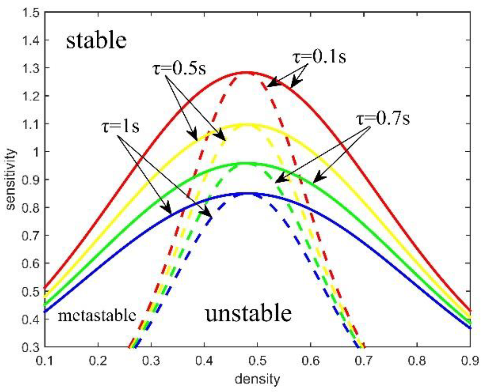
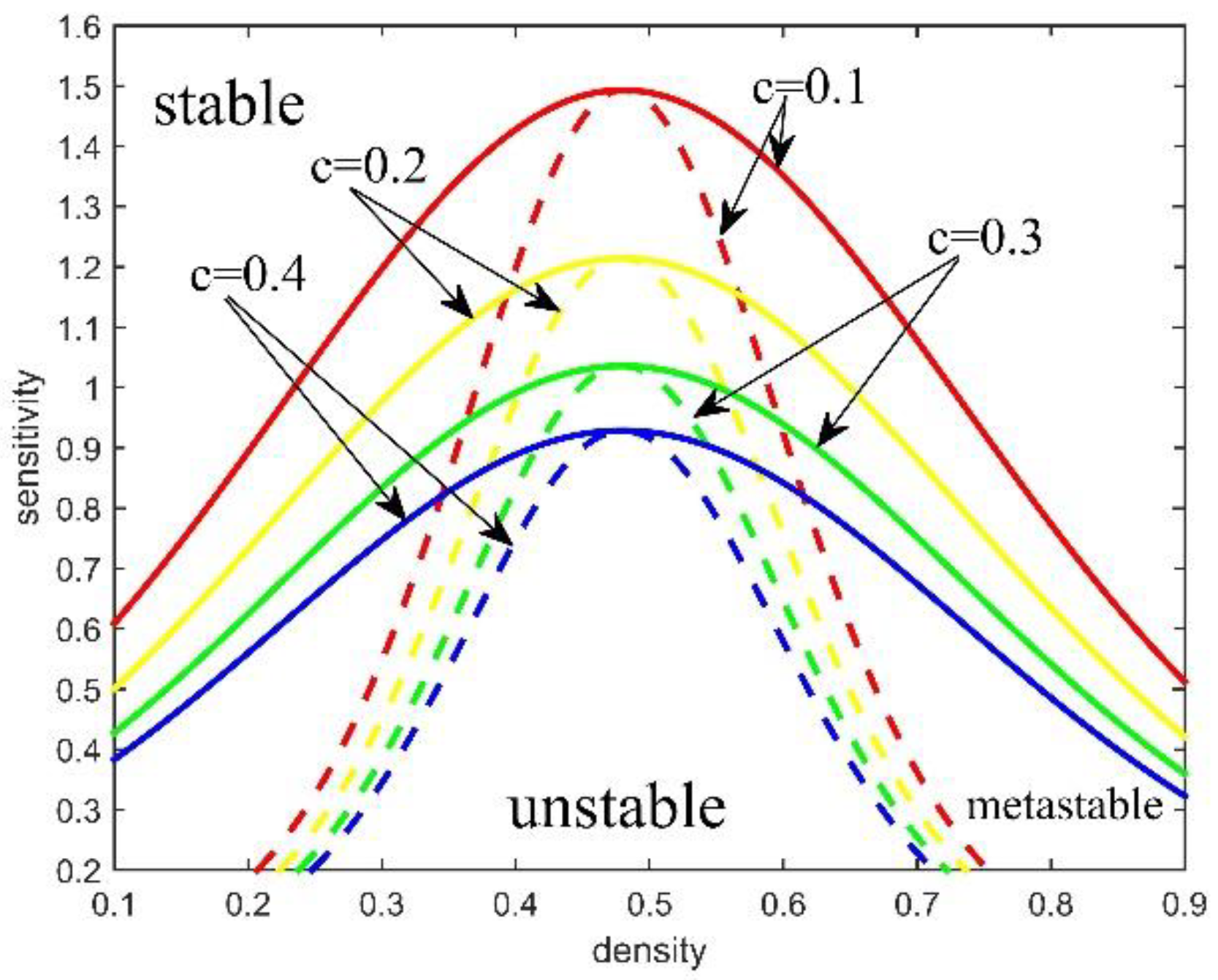
3.1. Linear Stability Analysis

The driver may suddenly accelerate or decelerate during driving, generating in a slight change in vehicle density, which is equivalent to adding a small disturbance to the overall stable traffic flow. The stability analysis mainly investigates the impact of small- and medium-sized disturbances on the overall traffic flow, so as to grasp the evolution mechanism of them with clarity, improve the stability of traffic flow and alleviate traffic congestion.

When the traffic flow attains a steady state, we believe that the density of vehicles in the traffic flow is uniform. That is to say, Equation (13) has the equilibrium solution demonstrated Equation (14).

$${\rho }_{j,m}\left(t\right) = {\rho }_0.$$

(14)

In the state of stable traffic flow, we assume that a certain traffic jam occurs at site $j,m$, which leads to the density of traffic flow at this location deviating from the steady density. Set the deviation quantity namely the small disturbance at this position as $y_{j,m}$, then the density at site $j,m$ is met in Equation (15).

$${\rho }_{j,m}\left(t\right) = {\rho }_0+y_{j,m}\left(t\right).$$

(15)

After that, we substitute Equation (15) into Equation (13) and rearrange it to get the Equation (16).

$$\begin{array}{l}{\partial }_t^2{y}_{j,m}\left(t\right) + a{\partial }_t{y}_{j,m}\left(t\right)\\ + a{c}^2{\rho }_0^2\left[\left(y_{j+1,m}\left(t\right) - y_{j,m}\left(t\right)\right)V^{\prime }\left({\rho }_0\right)\right]\\ + a{c}^2{\rho }_0^2\beta \tau \left[{\partial }_t\left(y_{j+1,m}\left(t\right) - y_{j,m}\left(t\right)\right)V^{\prime }\left({\rho }_0\right)\right]\\ + a{\left(1-c\right)}^2{\rho }_0^2\left[\left(y_{j,m+1}\left(t\right) - y_{j,m}\left(t\right)\right)V^{\prime }\left({\rho }_0\right)\right]\\ + a{\left(1-c\right)}^2{\rho }_0^2\beta \tau \left[{\partial }_t\left(y_{j,m+1}\left(t\right) - y_{j,m}\left(t\right)\right)V^{\prime }\left({\rho }_0\right)\right] = 0\end{array}.$$

(16)

where $V^{\prime }\left({\rho }_0\right) = \frac{\partial V\left(\rho \right)}{\partial \rho }\left|{}_{\rho = {\rho }_0}\right.$.

Next, since density waves travel at the same speed in both the west and south directions, we expand $y_{j,m}\left(t\right)$ into Fourier series. Then substituting the expansion equation $y_{j,m}\left(t\right) = \exp \left(ik\left(j+m\right) + zt\right)$ into Equation (16) to get the Equation (17) written as

$$z^2+az+a\left(c^2+{\left(1-c\right)}^2\right){\rho }_0^2\left[\left(e^{ik}-1\right)V^{\prime }\left({\rho }_0\right) + \beta \tau z\left(e^{ik}-1\right)V^{\prime }\left({\rho }_0\right)\right] = 0,$$

(17)

For simplicity, letting $z = z_1\left(ik\right) + z_2{\left(ik\right)}^2+\cdots$ and substituting it into Equation (17). For solving for $z_1$ and $z_2$, we rearrange the equation according to the coefficients of $ik$ and ${\left(ik\right)}^2$. Setting the coefficient of them equal to zero, we acquire $z_1$ demonstrated as Equation (18) and $z_2$ containing $z_1$. Finally substitute Equation (18) into $z_2$ obtain the following result.

$$z_1 = -\left(c^2+{\left(1-c\right)}^2\right){\rho }_0^2{V}^{\prime }\left({\rho }_0\right),$$

(18)

$$z_2 = -\left[\frac{1}{2}+\left(\frac{1}{a}+\beta \tau \right)\left(c^2+{\left(1-c\right)}^2\right){\rho }_0^2{V}^{\prime }\left({\rho }_0\right)\right]\left(c^2+{\left(1-c\right)}^2\right){\rho }_0^2{V}^{\prime }\left({\rho }_0\right).$$

(19)

If $z_2$ is a negative value, the uniform steady-state flow becomes unstable for long-wavelength modes. The steady state traffic flow remains steady when it is disturbed by a small amount, and there will be no traffic jam. When $z_2$ is a positive value, the uniform flow is stable. The system will be unstable after a period of evolution, resulting in the generation of time-travel stop wave. According to the above results and combined with the existing traffic flow stability theory, it is generally accepted that the steady-state flow becomes unstable when $z_2<0$. On the contrary, the traffic flow system would remain stable when $z_2>0$. In other words, the stability conditions have been satisfied. Thus, we achieve the curve of neutral stability as

$$a = -\frac{2\left(c^2+{\left(1-c\right)}^2\right){\rho }_0^2{V}^{\prime }\left({\rho }_0\right)}{1-2\left(c^2+{\left(1-c\right)}^2\right){\rho }_0^2{V}^{\prime }\left({\rho }_0\right)\beta \tau },$$

(20)

The stability condition, consequently, for uniform traffic flow, is illuminated as inequality Equation (21).

$$a>-\frac{2\left(c^2+{\left(1-c\right)}^2\right){\rho }_0^2{V}^{\prime }\left({\rho }_0\right)}{1-2\left(c^2+{\left(1-c\right)}^2\right){\rho }_0^2{V}^{\prime }\left({\rho }_0\right)\beta \tau },$$

(21)

When $c = 0$ or $1$, the model is one-dimensional lattice model with the consideration of driver predictive effect, and the stability condition is converted to inequality Equation (22).

$$a>-\frac{2{\rho }_0^2{V}^{\prime }\left({\rho }_0\right)}{1-2{\rho }_0^2{V}^{\prime }\left({\rho }_0\right)\beta \tau }.$$

(22)

The stability conditions of inequality Equation (22) are consistent with those obtained in the one-dimensional predictive effect model by Wang et al. [37], which proves the correctness of our theoretical analysis to some extent.

Figure 2 and Figure 3 show the neutral stability curves (dashed line) and coexisting curves (solid line) under the relevant parameters of the two factors investigated in this paper. As illustrated in the figure, above the coexisting curve and below the neutral stability curve are stable areas with smooth traffic and unstable areas with heavy traffic of traffic flow, respectively. Between these two curves is the metastable region of the vehicular system determined by the critical disturbance amplitude.

When parameters ${\rho }_0$, $\beta$ and $\tau$ are determined, we can obtain from Equation (20), the driver sensitivity coefficient $a$ increases as the fraction of eastbound cars $c$ increases if $0<c<0.5$ while $a$ decreases as $c$ increases if $0.5<c<1$. In addition, if $c$ is regarded as a function of $c$, $c = 0.5$ is the axis of symmetry of this function. In other words, the neutral stability curves determined by $c = C$ and $c = 1-C$$\left(0<c<1\right)$ coincide when other parameters are determined. Figure 2 display the curves for $c = 0.1$, $0.2$, $0.3$, $0.4$ with $\beta = 0.3$, $\tau = 0.4 \mathrm{s}$ and $v_{\max } = 2 \mathrm{m}/\mathrm{s}$. From this picture, we can see that the stability region increases with the increase of $c$$\left(0<c<0.5\right)$. This indicates that the uniform distribution of traffic flow will play an inhibitory role on traffic congestion.

Figure 3 demonstrates that the curves for $\tau = 0.1 \mathrm{s}$, $0.4 \mathrm{s}$, $0.7 \mathrm{s}$, $1 \mathrm{s}$ with $\beta = 0.3$, $c = 0.2$ and $v_{\max } = 2 \mathrm{m}/\mathrm{s}$. We can discover that with the increase of the predictive time $\tau$ stability region increases from this diagram. At this time, the probability of traffic congestion is greatly reduced. By observing the stability conditions of Equation (21), we can find that $\beta$ and $\tau$ have the same influence on $a$; in other words, the prediction weight $\beta$ also plays a vigorous role in the stability of traffic flow. To sum up, the predictive effect of drivers does curb traffic congestion.

3.2. Nonlinear Analysis

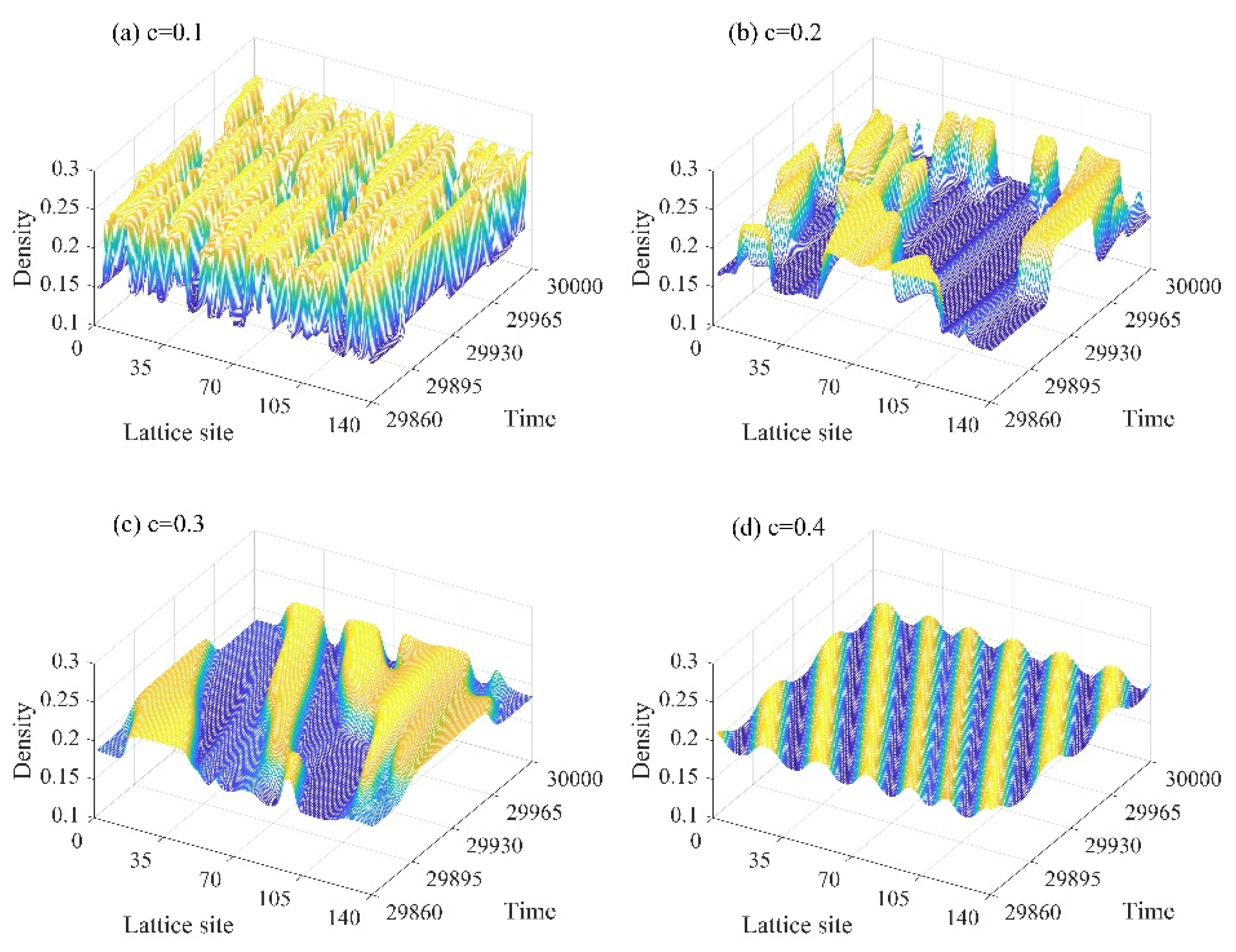
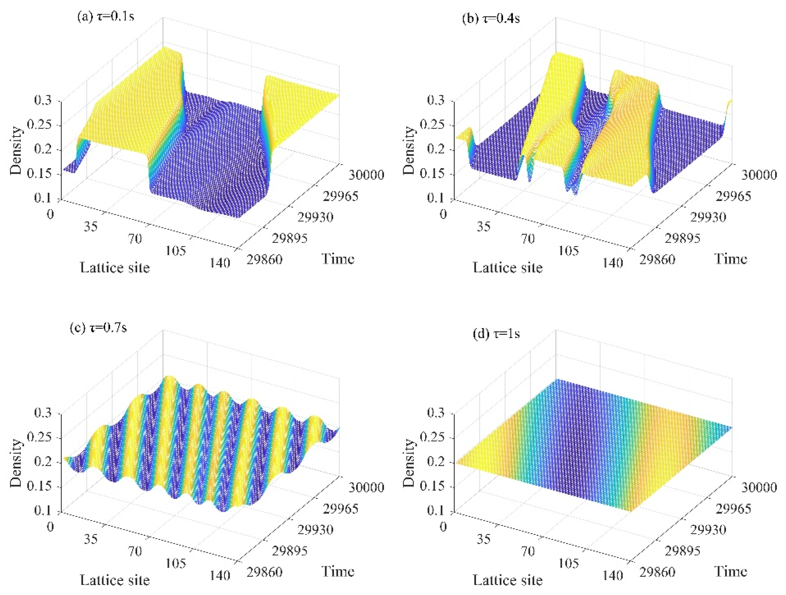
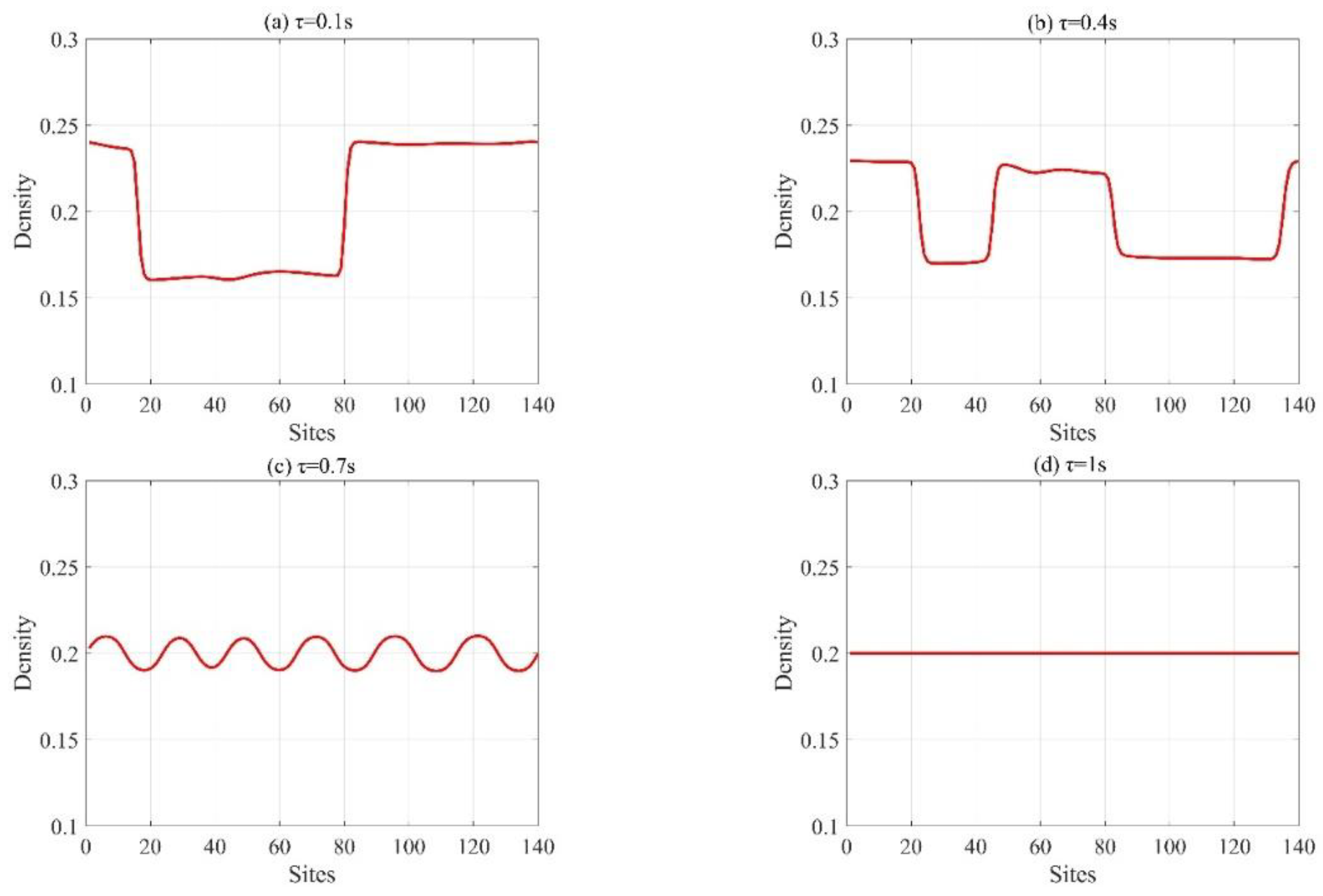
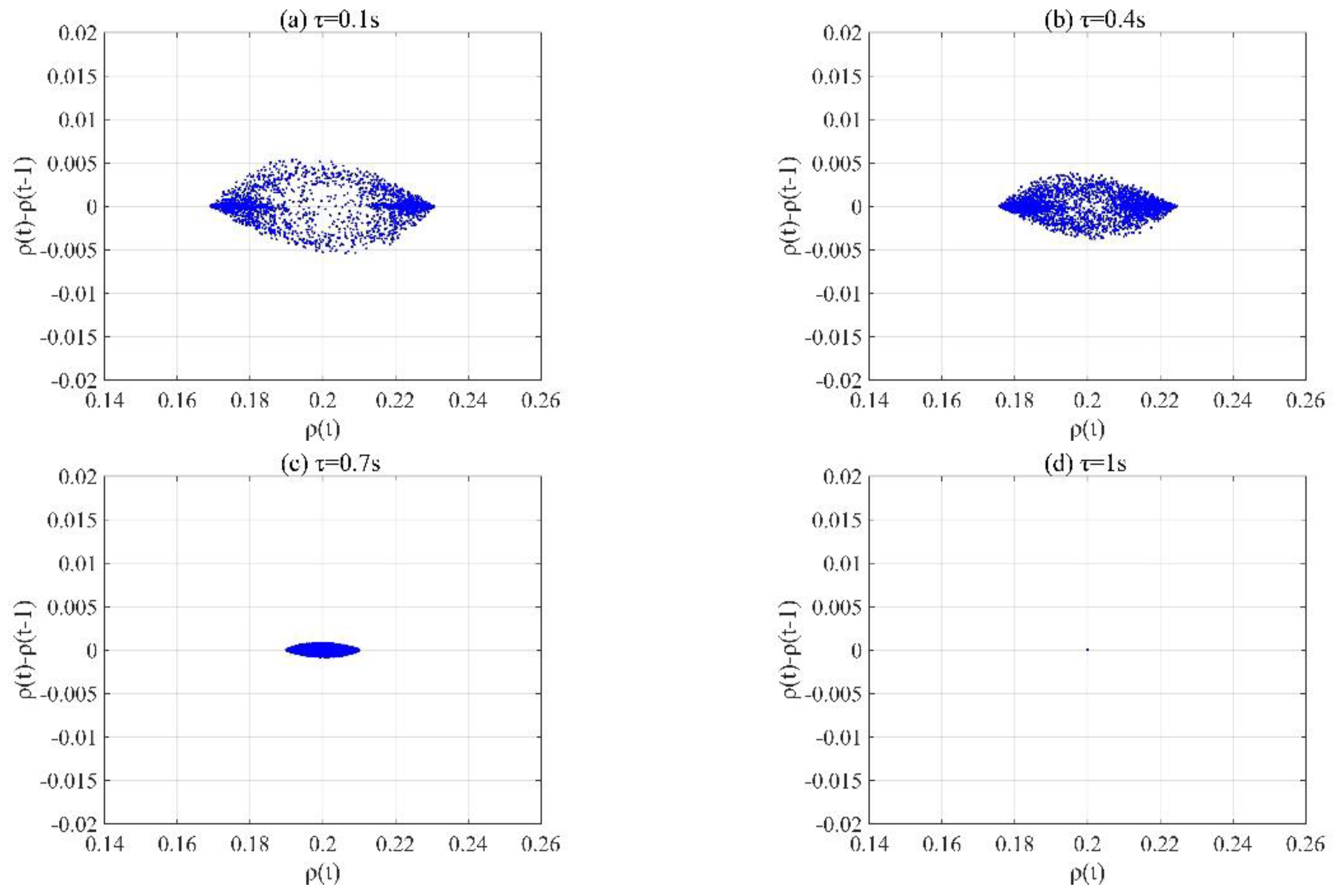
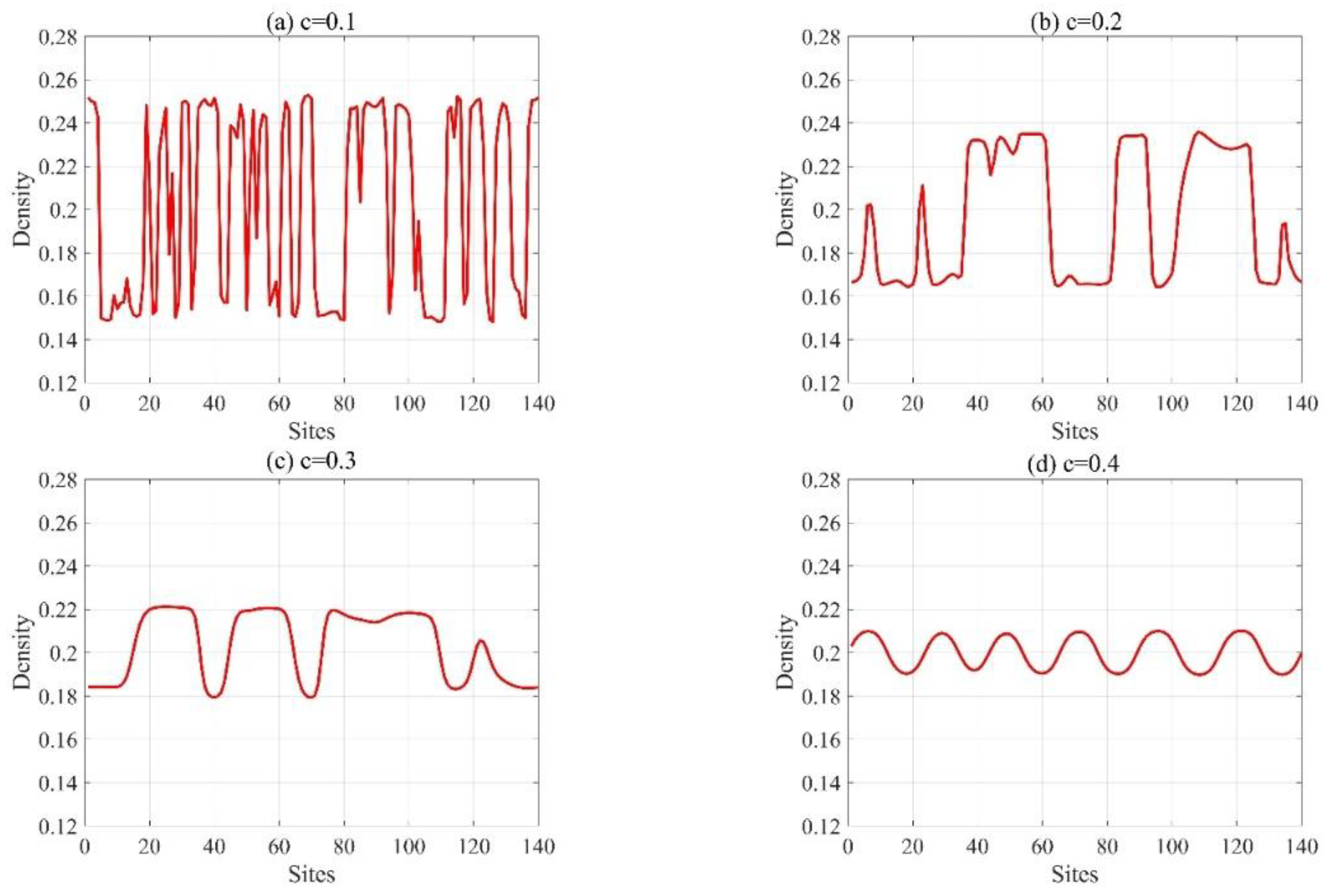
The nonlinear phenomenon of traffic flow is analyzed by considering the changing behavior of the time slowing variable and space slowing variable near the critical point $\left({\rho }_c,a_c\right)$ of the unstable traffic flow region. The slow variables of time and space $X$ and $T$ are imported respectively for a small positive scaling parameter $\epsilon \left(0<\epsilon <<1\right)$ as

$$X = \epsilon \left(j+m+bt\right), T = {\epsilon }^{3}t,$$

(23)

where $b$ means the undetermined parameters. Then we set the density of each lattice ${\rho }_{j,m}\left(t\right)$ to satisfy Equation (23).

$${\rho }_{j,m}\left(t\right) = {\rho }_c+\epsilon R(X,T).$$

(24)

According to the above Equations (23) and (24), each item in Equation (12) is expanded to the fifth term of $\epsilon$ by performing the Taylor expansion method. To make the expression simple and obvious, we set $\lambda = \left(c^2+{\left(1-c\right)}^2\right)$. Then, we can acquire the following expression:

$$\begin{array}{l}{\epsilon }^2\left[\left(ab+a\lambda {\rho }_c^2{V}^{\prime }\left({\rho }_c\right)\right){\partial }_{X}R\right]\\ + {\epsilon }^3\left[\left(b^2+\frac{a\lambda {\rho }_c^2{V}^{\prime }\left({\rho }_c\right)}{2}+a\lambda b\beta \tau {\rho }_c^2{V}^{\prime }\left({\rho }_c\right)\right){\partial }_X^{2}R\right]\\ + {\epsilon }^4\left[a{\partial }_{T}R + \left(\frac{a\lambda {\rho }_c^2{V}^{\prime }\left({\rho }_c\right)}{6}+\frac{a\lambda b\beta \tau {\rho }_c^2{V}^{\prime }\left({\rho }_c\right)}{2}\right){\partial }_X^{3}R+\frac{a\lambda {\rho }_c^2{V}^{‴}\left({\rho }_c\right)}{6}{\partial }_X{R}^3\right]\\ + {\epsilon }^5\left[\begin{array}{l}\left(2b+a\lambda \beta \tau {\rho }_c^2{V}^{\prime }\left({\rho }_c\right)\right){\partial }_T{\partial }_{X}R + \left(\frac{a\lambda {\rho }_c^2{V}^{\prime }\left({\rho }_c\right)}{24}+\frac{a\lambda b\beta \tau {\rho }_c^2{V}^{\prime }\left({\rho }_c\right)}{6}\right){\partial }_X^{4}R \\ + \left(\frac{a\lambda {\rho }_c^2{V}^{‴}\left({\rho }_c\right)}{12}+\frac{a\lambda b\beta \tau {\rho }_c^2{V}^{‴}\left({\rho }_c\right)}{6}\right){\partial }_X^2{R}^3\end{array}\right] = 0\end{array}.$$

(25)

where $V^{\prime }\left({\rho }_c\right) = \frac{\partial V\left(\rho \right)}{\partial \rho }\left|{}_{\rho = {\rho }_c}\right.$ and $V^{‴}\left({\rho }_c\right) = \frac{{\partial }^{3}V\left(\rho \right)}{\partial {\rho }^3}\left|{}_{\rho = {\rho }_c}\right.$.

Moreover, there is $a = \left(1-{\epsilon }^2\right)a_c$ at the unstable region near the critical point $\left({\rho }_c,a_c\right)$. Then, in order to simplify Equation (25), we set the coefficient of the quadratic term of $\epsilon$ equal to zero to obtain $b = -\lambda {\rho }_c^2{V}^{\prime }\left({\rho }_c\right)$. Furthermore, substituting $a = \left(1-{\epsilon }^2\right)a_c$ and $b = -\lambda {\rho }_c^2{V}^{\prime }\left({\rho }_c\right)$ into Equation (25), an evolutionary equation with only fourth and fifth terms of $\epsilon$ can be deduced as

$${\epsilon }^4(-g_1{\partial }_X^{3}R+g_2{\partial }_X{R}^3+{\partial }_{T}R)+{\epsilon }^5(g_4{\partial }_X^{4}R+g_5{\partial }_X^2{R}^3-g_3{\partial }_X^{2}R) = 0,$$

(26)

where the coefficients $g_i\left(1,2,\dots ,5\right)$ are shown as

$$g_1 = \frac{a\lambda {\rho }_c^2{V}^{\prime }\left({\rho }_c\right)}{6}+\frac{a\lambda b\beta \tau {\rho }_c^2{V}^{\prime }\left({\rho }_c\right)}{2},$$

(27)

$$g_2 = \frac{a{\rho }_c^2{V}^{‴}\left({\rho }_c\right)}{6},$$

(28)

$$g_3 = \frac{a\lambda {\rho }_c^2{V}^{\prime }\left({\rho }_c\right)}{2}+a\lambda b\beta \tau {\rho }_c^2{V}^{\prime }\left({\rho }_c\right),$$

(29)

$$g_4 = \frac{a\lambda {\rho }_c^2{V}^{\prime }\left({\rho }_c\right)}{24}+\frac{a\lambda b\beta \tau {\rho }_c^2{V}^{\prime }\left({\rho }_c\right)}{6},$$

(30)

$$g_5 = \frac{a\lambda {\rho }_c^2{V}^{‴}\left({\rho }_c\right)}{12}+\frac{a\lambda b\beta \tau {\rho }_c^2{V}^{‴}\left({\rho }_c\right)}{6},$$

(31)

For the sake of deriving the standard mKdV equation, we make the following equivalent substitution.

$$T = \frac{1}{g_1}{T}^{\prime },R = \sqrt{\frac{g_1}{g_2}}{R}^{\prime }.$$

(32)

Subsequently, substituting Equation (32) into Equation (26) and adding the correction term of $O\left(\epsilon \right)$ into the model, the Equation (26) is turned into Equation (33).

$${\partial }_{T^{\prime }}{R}^{\prime } = {\partial }_X^3{R}^{\prime }-{\partial }_X{R^{\prime }}^3+\epsilon M\left[R^{\prime }\right].$$

(33)

where $M\left[R^{\prime }\right] = \frac{g_3}{g_1}{\partial }_X^2{R}^{\prime }+\frac{g_4}{g_1}{\partial }_X^4{R}^{\prime }+\frac{g_5}{g_2}{\partial }_X^2{R^{\prime }}^3$ and this item means the higher order infinitesimal term.

Additionally, after ignoring the correction term $O\left(\epsilon \right)$, the kink-antikink density wave solution of the mKdV equation is Equation (34).

$$R_0^{\prime }\left(X,T^{\prime }\right) = \sqrt{s}\tanh \left(\sqrt{\frac{s}{2}}\left(X-s{T}^{\prime }\right)\right),$$

(34)

where $s$ denotes the propagation speed of the above kink-antikink solitary wave.

Then, the following condition must be satisfied to help us obtain the value of the propagation velocity $s$ for the kink solution

$$\left(R_0^{\prime },M\left[R_0^{\prime }\right]\right) = {\displaystyle {\int }_{-\infty }^{+\infty }d{X}^{\prime }{R}_0^{\prime }M\left[R_0^{\prime }\right]} = 0.$$

(35)

where $M\left[R_0^{\prime }\right] = M\left[R^{\prime }\right]$, we get the general solution form of velocity $s$ through solving the Equation (33) as

$$s = \frac{5g_2{g}_3}{2g_2{g}_4-3g_1{g}_5},$$

(36)

By replacing the velocity $s$ in Equation (32) with Equation (34), the following equation can be obtained.

$$R(X,T) = \sqrt{\frac{g_{1}s}{g_2}}\tanh \left(\sqrt{\frac{s}{2}}\left(X-s{g}_{1}T\right)\right),$$

(37)

Since then, the general kink-antikink solution of the mKdV equation can be expressed as Equation (38).

$${\rho }_j(t) = {\rho }_c+\epsilon \sqrt{\frac{g_{1}s}{g_2}}\tanh \left(\sqrt{\frac{s}{2}}\left(X-s{g}_{1}T\right)\right).$$

(38)

Evidently, the amplitude $A$ of the density soliton is

$$A = \epsilon \sqrt{\frac{g_{1}s}{g_2}}.$$

(39)

Generally speaking, we commonly exert ${\rho }_j = {\rho }_c-A$ and ${\rho }_j = {\rho }_c+A$ to describe the densities of the freely moving phase and congested phase, respectively. This kink-antikink soliton represents the coexistence phases containing the freely moving phase with low density and the congested phase with high density.

4. Results

For convenience of numerical simulation, the Equation (12) is rewritten into the following difference form:

$$\begin{array}{l}{\rho }_{j,m}\left(t+2\mathsf{\Delta }t\right) - 2{\rho }_{j,m}\left(t+\mathsf{\Delta }t\right) + {\rho }_{j,m}\left(t\right) + a\mathsf{\Delta }t\left({\rho }_{j,m}\left(t+\mathsf{\Delta }t\right) - {\rho }_{j,m}\left(t\right) \right)\\ + a\mathsf{\Delta }{t}^2{c}^2{\rho }_0^2\left[\begin{array}{l}V\left({\rho }_{j+1,m}\left(t\right)\right) + \beta \tau \left(\frac{{\rho }_{j+1,m}\left(t + \mathsf{\Delta }t\right) - {\rho }_{j+1,m}\left(t\right)}{\mathsf{\Delta }t}\right)V^{\prime }\left({\rho }_{j+1,m}\left(t\right) \right)\\ - \left(V\left({\rho }_{j,m}\left(t\right)\right) + \beta \tau \left(\frac{{\rho }_{j,m}\left(t + \mathsf{\Delta }t\right) - {\rho }_{j,m}\left(t\right)}{\mathsf{\Delta }t}\right)V^{\prime }\left({\rho }_{j,m}\left(t\right)\right)\right)\end{array}\right]\\ + a\mathsf{\Delta }{t}^2{\left(1-c\right)}^2{\rho }_0^2\left[\begin{array}{l}V\left({\rho }_{j,m+1}\left(t\right)\right) + \beta \tau \left(\frac{{\rho }_{j,m+1}\left(t + \mathsf{\Delta }t\right) - {\rho }_{j,m+1}\left(t\right)}{\mathsf{\Delta }t}\right)V^{\prime }\left({\rho }_{j,m+1}\left(t\right) \right)\\ - \left(V\left({\rho }_{j,m}\left(t\right)\right) + \beta \tau \left(\frac{{\rho }_{j,m}\left(t + \mathsf{\Delta }t\right) - {\rho }_{j,m}\left(t\right)}{\mathsf{\Delta }t}\right)V^{\prime }\left({\rho }_{j,m}\left(t\right)\right)\right)\end{array}\right] = 0\end{array}.$$

(40)

We select a $140\times 140$ grid to take different values of the corresponding parameters, and conduct numerical simulation to get the spatial-temporal evolution diagram and spatial distribution diagram of density wave after $t = \text{10,300} \mathrm{s}$.

Figure 4 shows the space-time evolution of density waves with different values of with $a = 0.86$, ${\rho }_c = 0.2$, and $\tau = 0.7 \mathrm{s}$. When we set $c = 0.1,0.2,0.3,0.4$, there are torque–reverse torque density waves in all four figures of Figure 4, because there is a certain degree of congestion on the roads and the stability condition is not satisfied. Nevertheless, since the frequency and amplitude of the four images are gradually decreasing, we can conclude that the density wave tends to be stable gradually with the increase of $c$. In other words, the increase of the proportion of eastbound vehicles will play a constructive role in the stability of traffic flow and restrain the occurrence of traffic congestion.

Figure 5 depicts the density wave spatial distribution diagram corresponding to Figure 4, namely the instantaneous traffic flow distribution on each lattice at $t = \text{10,300} \mathrm{s}$. Figure 5 can more briefly and clearly reflect the variation rule of the amplitude and frequency of density wave with the parameter $c$. From these changes, we can see that the increase of parameter $c$ makes the density wave gradually tend to be stable, that is to say, the decrease of eastbound vehicles will deteriorate the traffic congestion.

Figure 6 is the plots of density versus density difference at the $\left(\text{100,100}\right)$ lattice corresponding to Figure 4. With the increase of $c$, the loop area gradually decreases, which further verifies the above conclusion.

Figure 7 clearly illustrates the influence of the driver’s prediction effect on the time evolution of density wave with different values of $\tau$ which are the driver’s prediction time. Other parameters are selected as $a = 0.86$, ${\rho }_c = 0.2$, and $c = 0.4$. First of all, we can find intuitively that the first two pictures in Figure 7 have relatively large amplitudes, which means the traffic is relatively unstable. Then we can see that the amplitude of the latter one changes significantly and that the last one is a plane with almost no fluctuations. Thereby, the density wave becomes more and more stable as $\tau$ increases and the increase of prediction time will reduce the occurrence of traffic flow instability phenomena.

What is described in Figure 8 is the two-dimensional density spatial distribution diagram corresponding to Figure 8. It can be clearly seen from the figure that the amplitude of density wave becomes smaller and smaller with the increase of the predicted time $\tau$ until it finally becomes a straight line with almost no oscillation, which means that the traffic flow reaches a stable state. In conclusion, the predictive effect will promote the stability of traffic flow and will inhibit the occurrence of traffic jams.

Similar to Figure 6, Figure 9 is the plots of density versus density difference at the $\left(\text{100,100}\right)$ lattice corresponding to Figure 7. With the increase of $\tau$, the area of loop obviously decreases and eventually becomes an solitary point, which is consistent with the conclusion obtained above.

5. Conclusions

On the foundation of the discrete macro model proposed by Nagatani [16], this paper imports the driver’s prediction effect, and obtains a new two-dimensional lattice hydrodynamic model. Through theoretical analysis and numerical simulation of the model, the influence of the prediction effect on the stability of two-dimensional traffic flow is investigated. The results of linear analysis illustrate that the traffic becomes smoother with the gradual increase of the proportion of eastbound vehicles or the driver’s prediction effect time. Furthermore, the mKdV equation and its kink-antikink solution are derived when approaching the critical point in the unstable region. In addition, we plot phase diagrams to demonstrate the effect of corresponding parameters on traffic flow stability. By comparison, we find that the numerical simulation results are in agreement with the theoretical analysis. They unanimously manifest that a reasonable proportion of eastbound vehicles and effective prediction of drivers will reduce the occurrence of traffic congestion. In general, the two-dimensional model established in this paper can well reflect the evolution of the prediction effect on the vehicle moving forward and blocking in the actual traffic. The novel model we proposed provides a theoretical basis for solving the problem of traffic congestion and traffic flow prediction and control in reality.

References

1. Yu, S.; Shi, Z. Analysis of car-following behaviors considering the green signal countdown device. Nonlinear Dyn. 2015, 82, 731–740. [Google Scholar] [CrossRef]
2. Zhu, W.; Li, D. A new car-following model for autonomous vehicles flow with mean expected velocity field. Phys. A Stat. Mech. Appl. 2018, 492, 2154–2165. [Google Scholar]
3. Zhu, W.; Zhang, H. Analysis of mixed traffic flow with human-driving and autonomous cars based on car-following model. Phys. A Stat. Mech. Appl. 2018, 496, 274–285. [Google Scholar] [CrossRef]
4. Ou, H.; Tang, T. An extended two-lane car-following model accounting for inter-vehicle communication. Phys. A Stat. Mech. Appl. 2018, 495, 260–298. [Google Scholar] [CrossRef]
5. Ngoduy, D. Effect of the car-following combinations on the instability of heterogeneous traffic flow. Transp. B Transp. Dyn. 2015, 3, 44–58. [Google Scholar] [CrossRef]
6. Zhu, M.; Wang, X. Human-like autonomous car-following model with deep reinforcement learning. Transp. Res. Part C Emerg. Technol. 2018, 97, 348–368. [Google Scholar] [CrossRef] [Green Version]
7. Ma, L.; Qu, S. A sequence to sequence learning based car-following model for multi-step predictions considering reaction delay. Transp. Res. Part C Emerg. Technol. 2020, 120, 102785. [Google Scholar] [CrossRef]
8. An, S.; Xu, L.; Qian, L. Car-following model for autonomous vehicles and mixed traffic flow analysis based on discrete following interval. Phys. A Stat. Mech. Appl. 2020, 560, 125246. [Google Scholar] [CrossRef]
9. Xue, Y.; Zhang, Y.; Fan, D. An extended macroscopic model for traffic flow on curved road and its numerical simulation. Nonlinear Dyn. 2019, 95, 3295–3307. [Google Scholar] [CrossRef]
10. Peng, G.; Song, W.; Peng, Y. A novel macro model of traffic flow with the consideration of anticipation optimal velocity. Phys. A Stat. Mech. Appl. 2014, 398, 76–82. [Google Scholar] [CrossRef]
11. Cheng, R.; Ge, H.; Wang, J. An extended continuum model accounting for the driver’s timid and aggressive attributions. Phys. Lett. A 2017, 381, 1302–1312. [Google Scholar] [CrossRef]
12. Cheng, R.; Wang, Y. An extended lattice hydrodynamic model considering the delayed feedback control on a curved road. Phys. A Stat. Mech. Appl. 2019, 513, 510–517. [Google Scholar] [CrossRef]
13. Zhai, Q.; Ge, H.; Cheng, R. An extended continuum model considering optimal velocity change with memory and numerical tests. Phys. A Stat. Mech. Appl. 2018, 490, 774–785. [Google Scholar]
14. Cheng, R.; Ge, H.; Wang, J. The nonlinear analysis for a new continuum model considering anticipation and traffic jerk effect. Appl. Math. Comput. 2018, 332, 493–505. [Google Scholar]
15. Davoodi, N.; Soheili, A.; Hashemi, S. A macro-model for traffic flow with consideration of driver’s reaction time and distance. Nonlinear Dyn. 2016, 83, 1621–1628. [Google Scholar] [CrossRef]
16. Nagatani, T. Modified KdV equation for jamming transition in the continuum models of traffic. Phys. A Stat. Mech. Appl. 1998, 261, 599–607. [Google Scholar] [CrossRef]
17. Nagatani, T. Jamming transition and the modified Kortweg-de Vries equation in a two-lane traffic flow. Phys. A Stat. Mech. Appl. 1999, 265, 297–310. [Google Scholar] [CrossRef]
18. Nagatani, T. TDGL and MKdV equations for jamming transition in the lattice models of traffic. Phys. A Stat. Mech. Appl. 1999, 264, 581–592. [Google Scholar] [CrossRef]
19. Cao, J.; Shi, Z. Analysis of a novel two-lane lattice model on a gradient road with the consideration of relative current. Commun. Nonlinear Sci. Numer. Simul. 2016, 33, 1–18. [Google Scholar] [CrossRef]
20. Peng, G.; Kuang, H.; Qing, L. A new lattice model of traffic flow considering driver’s anticipation effect of the traffic interruption probability. Phys. A Stat. Mech. Appl. 2018, 507, 374–380. [Google Scholar] [CrossRef]
21. Zhao, H.; Xia, D.; Yang, S. The delayed-time effect of traffic flux on traffic stability for two-lane freeway. Phys. A Stat. Mech. Appl. 2020, 105, 106308. [Google Scholar] [CrossRef]
22. Wang, T.; Cheng, R.; Ge, H. Analysis of a novel two-lane lattice hydrodynamic model considering the empirical lane changing rate and the self-stabilization effect. IEEE Access 2019, 540, 123066. [Google Scholar] [CrossRef]
23. Wang, J.; Sun, F.; Ge, H. An improved lattice hydrodynamic model considering the driver’s desire of driving smoothly. Phys. A Stat. Mech. Appl. 2019, 515, 119–129. [Google Scholar] [CrossRef]
24. Wu, X.; Zhao, X.; Song, H.; Xin, S.; Yu, S. Effects of the prevision relative velocity on traffic dynamics in the ACC strategy. Phys. A Stat. Mech. Appl. 2019, 515, 192–198. [Google Scholar] [CrossRef]
25. Bando, M.; Hasebe, K.; Nakayama, A.; Shibata, A.; Sugiyama, Y. Dynamical model of traffic congestion and numerical simulation. Phys. Rev. E 1995, 51, 1035–1042. [Google Scholar] [CrossRef]
26. Zhu, W.; Yu, R. Nonlinear analysis of traffic flow on a gradient highway. Phys. A Stat. Mech. Appl. 2012, 391, 964–965. [Google Scholar] [CrossRef]
27. Gupta, A.; Sharma, S.; Redhu, P. Analyses of lattice traffic model on a Gradient highway. Commun. Theor. Phys. 2014, 62, 393–404. [Google Scholar] [CrossRef]
28. Zhou, J.; Shi, Z.; Cao, J. An extended traffic flow model on a gradient highway with the consideration of the relative velocity. Nonlinear Dyn. 2014, 78, 1765–1779. [Google Scholar] [CrossRef]
29. Zhang, G. The self-stabilization effect of lattice’s historical flow in a new lattice hydrodynamic model. Nonlinear Dyn. 2018, 91, 809–817. [Google Scholar] [CrossRef]
30. Peng, G.; Zhao, H.; Li, X. The impact of self-stabilization on traffic stability considering the current lattice’s historic flux for two-lane freeway. Phys. A Stat. Mech. Appl. 2019, 515, 31–37. [Google Scholar] [CrossRef]
31. Wang, T.; Gao, Z.; Zhao, X. Flow difference effect in the two-lane lattice hydrodynamic model. Chin. Phys. B 2012, 7, 211–219. [Google Scholar] [CrossRef]
32. Gupta, A.; Redhu, P. Analysis of a modified two-lane lattice model by considering the density difference effect. Commun. Nonlinear Sci. Numer. Simul. 2014, 19, 1600–1610. [Google Scholar] [CrossRef]
33. Nagatani, T. Jamming transition in a two-dimensional traffic flow model. Phys. Rev. E 1999, 59, 4857–4864. [Google Scholar] [CrossRef] [PubMed] [Green Version]
34. Redhu, P.; Gupta, A. The role of passing in a two-dimensional network. Nonlinear Dyn. 2016, 86, 389–399. [Google Scholar] [CrossRef]
35. Liu, Y.; Wong, C. A two-dimensional lattice hydrodynamic model considering shared lane marking. Phys. Lett. A 2020, 384, 126668. [Google Scholar] [CrossRef]
36. Li, L.; Cheng, R.; Ge, H. New feedback control for a novel two-dimensional lattice hydrodynamic model considering driver’s memory effect. Phys. A Stat. Mech. Appl. 2021, 561, 125295. [Google Scholar] [CrossRef]
37. Wang, T.; Zang, R.; Xu, K.; Zhang, J. Analysis of predictive effect on lattice hydrodynamic traffic flow model. Phys. A Stat. Mech. Appl. 2019, 526, 120711. [Google Scholar] [CrossRef]
38. Zhang, J.; Xu, K.; Li, S.; Wang, T. A new two-lane lattice hydrodynamic model with the introduction of driver’s predictive effect. Phys. A Stat. Mech. Appl. 2020, 551, 124249. [Google Scholar] [CrossRef]
39. Kaur, D.; Sharma, S. The impact of the predictive effect on traffic dynamics in a lattice model with passing. Eur. Phys. J. B Condens. Matter Complex Syst. 2020, 93, 35. [Google Scholar] [CrossRef]
Figure 1. Schematic model of traffic flow on a two-dimensional highway.
Mathematics 09 02464 g001
Figure 2. Phase diagrams in the density-sensitivity space for different c .
Mathematics 09 02464 g002
Figure 3. Phase diagrams in the density-sensitivity space for different τ .
Mathematics 09 02464 g003
Figure 4. Space–time evolution of density under different value of parameter c .
Mathematics 09 02464 g004
Figure 5. Density profile at t   =   10,300   s corresponding to Figure 4.
Mathematics 09 02464 g005
Figure 6. Plots of density versus density difference corresponding to Figure 4.
Mathematics 09 02464 g006
Figure 7. Space–time evolution of density under different value of parameter τ .
Mathematics 09 02464 g007
Figure 8. Density profile at t   =   10,300   s corresponding to Figure 7.
Mathematics 09 02464 g008
Figure 9. Plots of density versus density difference corresponding to Figure 7.
Mathematics 09 02464 g009
Publisher’s Note: MDPI stays neutral with regard to jurisdictional claims in published maps and institutional affiliations.