
Geary’s c and Spectral Graph Theory


School of Informatics and Data Science, Hiroshima University, 1-2-1 Kagamiyama, Higashi-Hiroshima 739-8525, Japan
Mathematics 2021, 9(19), 2465; https://doi.org/10.3390/math9192465
Submission received: 6 September 2021
/
Revised: 22 September 2021
/
Accepted: 22 September 2021
/
Published: 3 October 2021
(This article belongs to the Section D1: Probability and Statistics)
Abstract
:Spatial autocorrelation, of which Geary’s c has traditionally been a popular measure, is fundamental to spatial science. This paper provides a new perspective on Geary’s c. We discuss this using concepts from spectral graph theory/linear algebraic graph theory. More precisely, we provide three types of representations for it: (a) graph Laplacian representation, (b) graph Fourier transform representation, and (c) Pearson’s correlation coefficient representation. Subsequently, we illustrate that the spatial autocorrelation measured by Geary’s c is positive (resp. negative) if spatially smoother (resp. less smooth) graph Laplacian eigenvectors are dominant. Finally, based on our analysis, we provide a recommendation for applied studies.
Keywords:
spatial autocorrelation; Geary’s c; spectral graph theory; graph Laplacian; graph Laplacian quadratic form; graph Fourier transform; graph Laplacian eigenvalues; graph Laplacian eigenvectors; Pearson’s correlation coefficient; path graph; discrete cosine transformMSC:
62H11; 05C50JEL Classification:
C21; C221. Introduction
Spatial autocorrelation is fundamental to spatial science (Getis [1]). This is because it describes the similarity between signals on adjacent vertices. Strong positive (resp. negative) spatial autocorrelation occurs when most signals on adjacent vertices take similar (resp. dissimilar) values. If such clear tendencies do not exist, spatial autocorrelation is weak. Geary’s [2] c, which is a spatial generalization of the von Neumann [3] ratio, has traditionally been a popular measure of spatial autocorrelation. There exists
See, e.g., de Jong et al. [4] (Equation (6)). Herein, we provide a new perspective on Geary’s c. We discuss this using concepts from spectral graph theory/linear algebraic graph theory and, based on our analysis, provide a recommendation for applied studies.
To present our contributions more precisely, let us clarify the graph considered herein. Let , where , denote an undirected graph without loops and multiple edges. We assume that n (the number of vertices) and m (the number of edges) are such that and , respectively. Then, m satisfies . For , let
and . Then, for , , , if , and . Accordingly, is a non-negative, symmetric, hollow, and nonzero matrix.
Example 1.
As an example of , consider the graph such that and . See Figure 1, which depicts . In this case, given that and do not belong to E, the corresponding , denoted by , is
which is a non-negative, symmetric, hollow, and nonzero matrix.
Let denote the observation (signal) on the vertex i for such that , where . Following Cliff and Ord [5,6,7,8], Geary’s c is defined as
where denotes the sum of all for , i.e., , which is positive by assumption. Note that, as stated, Geary’s c is a spatial generalization of the von Neumann [3] ratio:
We briefly describe this in the Appendix A.14.
Let , where for , and
which is referred to as graph Laplacian. By assumption, is a symmetric matrix.
Example 2.
As an example of , we show , which denotes the graph Laplacian of . That is,
which is a symmetric matrix.
As is a real symmetric matrix, it can be decomposed as
where is an orthogonal matrix and such that . Concerning the eigenvalues of , we assume .
Remark 1.
We note that by assuming we exclude the case such that . Then, it follows that
We exclude it because in this case Geary’s c equals one for any . For more details, see the Appendix A.1.
In spectral graph theory/linear algebraic graph theory, the following linear transformation:
where , is referred to as graph Fourier transform of . In addition, and for are referred to as graph Laplacian eigenvalues and graph Laplacian eigenvectors, respectively (see Hammond et al. [9] and Shuman et al. [10]). Let
Then, given , can be represented as a linear combination of graph Laplacian eigenvectors, , as follows:
Moreover, we have
which represents Parseval’s identity in the graph Fourier transform, see, e.g., Shuman et al. [11]. (Proof of (11) is provided in the Appendix A.2).
Remark 2.
(i) Harvey [12] (Equation (2.13)) represents Parseval’s identity in the Fourier representation of time series, which can be regarded as a special case of (11). See also Anderson [13] (Section 4.2.2). in Anderson [13] (Equations (14) and (21)) corresponds to in (6) for the case in which equals in Strang [14] (p. 136). (ii) The discrete cosine transform developed by Ahmed et al. [15] is an example of graph Fourier transform. For more details, see Appendix A.14.
Let denote the vector of the standard scores of :
where s denotes the sample standard deviation of , i.e., the positive square root of , and denote the graph Fourier transform of by :
Now, we are ready to state our contributions. As stated, this paper reconsiders Geary’s c using concepts from spectral graph theory. Our contributions herein are twofold.
- We present three types of representations for it. As the first type of representation, we give two matrix form representations that use graph Laplacian . As the second type of representation, we express it using and . Recall that they are the graph Fourier transform of and , respectively. As the third type of representation, we show its expression using squared Pearson’s correlation coefficients between and for .
- We illustrate that the spatial autocorrelation measured by Geary’s c is positive (resp. negative) if spatially smoother (resp. less smooth) graph Laplacian eigenvectors are dominant. Here, we note that is spatially smoother than for .
2. Preliminaries
2.1. Some Notations
Let , be the identity matrix of order n, denote the ith column of for , i.e., , and . Note that is the orthogonal projection matrix to the orthogonal complement of the space spanned by . For a vector , . Let , , and . For a vector , denote Pearson’s correlation coefficient between and by :
2.2. Key Preliminary Results for L
In this section, we provide key preliminary results for in (5).
First, given that is a symmetric matrix, satisfies
(Proof of (14) is provided in the Appendix A.3). Given that for , (14) leads to , from which we have for . (See also (18) and (19)).
In addition, it follows that
which implies that is an eigenpair of . Combining these results, we obtain , , and
We note that (16) is natural because belong to the orthogonal complement of the space spanned by .
Moreover, given that is a symmetric matrix such that , it follows that , which leads to
Finally, we have the following result.
Lemma 1.
Let for and be an matrix such that , where for . (Observe that ). Then, it follows that
where denotes an n-dimensional column vector.
Proof.
See the Appendix A.4. □
Example 3
(Example of ). Denote corresponding to by . Given , is a matrix such that
and thus we have
where for , and
Given and , from Lemma 1, we immediately have the following inequalities:
As illustrated in (21), defined in Lemma 1 may be regarded as a spatial differencing matrix. Thus, (22) implies that the ith graph Laplacian eigenvector, , is spatially smoother than the th graph Laplacian eigenvector, , for .
Remark 3.
(i) in (18) is referred to as graph Laplacian quadratic form of . In machine learning and statistics, use of graph Laplacian regularized filtering is becoming popular, see, e.g., Shuman et al. [10], Dong et al. [16], and Ricaud et al. [17]. (ii) As illustrated in (20), if , then , from which the corresponding column of is .
3. Three Types of Representations for Geary’s
In this section, we present three types of representations for Geary’s c: In Section 3.1, we show that it can be represented using . In Section 3.2, we show that it can be expressed using and . In Section 3.3, we show that it can be expressed using for . Subsequently, in Section 3.4, we clarify the relationship between , , and for .
3.1. Graph Laplacian Representation
Geary’s c in (3) can be expressed in matrix notation as follows.
Proposition 1.
(i) Geary’s c can be represented using as
(ii) Geary’s c can also be represented using very succinctly as
Proof.
See the Appendix A.5. □
Remark 4.
3.2. Graph Fourier Transform Representation
From (11), we have
In addition, given , we have
Likewise, Geary’s c can also be represented as
We summarize the properties obtained above in the following proposition.
Proposition 2.
(i) Let and for . Then, Geary’s c can be expressed using as
where both and are weighted averages of . In addition, satisfy
(ii) Let for . Then, Geary’s c can be expressed using as
and it is a weighted average of , which are non-negative. In addition, satisfy
Proof.
See the Appendix A.6. □
Remark 5.
(i) Given , we have
We note that the bounds of Geary’s c given by (35) were derived by de Jong et al. [4]. In addition, given that by assumption, it follows that
(ii) Let . Then, given , (32) can be rewritten as
Thus, c is also a weighted average of .
From Proposition 2, we have the following results.
Corollary 1.
It follows that
and
Proof.
See the Appendix A.7. □
Corollary 1 implies that plotting or is valuable for detecting spatial autocorrelation in .
3.3. Pearson’s Correlation Coefficient Representation
In this section, we express Geary’s c using Pearson’s correlation coefficient.
Denote Geary’s c for the case in which equals by :
Then, we have the following results.
Lemma 2.
can be expressed using as follows:
which thus satisfy and .
Proof.
See the Appendix A.8. □
In addition, we have the following result.
Lemma 3.
equals for .
Proof.
See the Appendix A.9. □
Then, given Lemmata 2 and 3, we have the following representation of Geary’s c.
Proposition 3.
For , Geary’s c can be expressed using Pearson’s correlation coefficients as
In addition, such correlation coefficients satisfy .
Proof.
See the Appendix A.10. □
Remark 7.
From Proposition 3, we have the following results.
Corollary 2.
For , it follows that
Corollary 2 implies that plotting is also valuable for detecting spatial autocorrelation in .
3.4. Some Remarks
Here, we clarify the relationship between , , and for . They are related as
for . Therefore, , , and provide essentially the same information. Nevertheless, among them, we prefer to and . This is because it satisfies
and thus its distribution appears similar to probability distribution.
4. An Illustration of When Geary’s Becomes Greater or Lesser Than One
In this section, we illustrate that Geary’s c becomes greater (resp. lesser) than one if spatially smoother (resp. less smooth) graph Laplacian eigenvectors are dominant. In other words, we show that the spatial autocorrelation measured by Geary’s c is positive (resp. negative) if spatially smoother (resp. less smooth) graph Laplacian eigenvectors are dominant. Recall that, from (22), is spatially smoother than for .
Other than these, concerning , we have the following results.
Lemma 4.
It follows that
Proof.
See the Appendix A.11. □
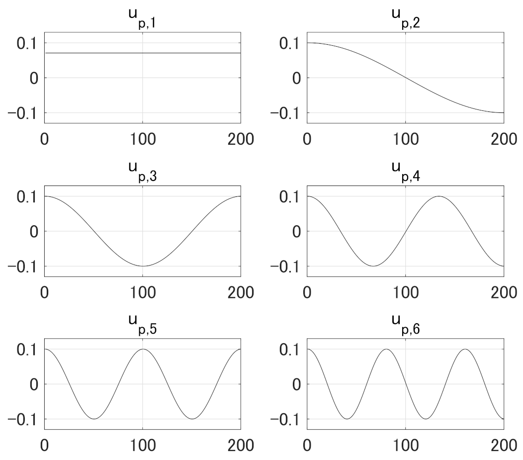
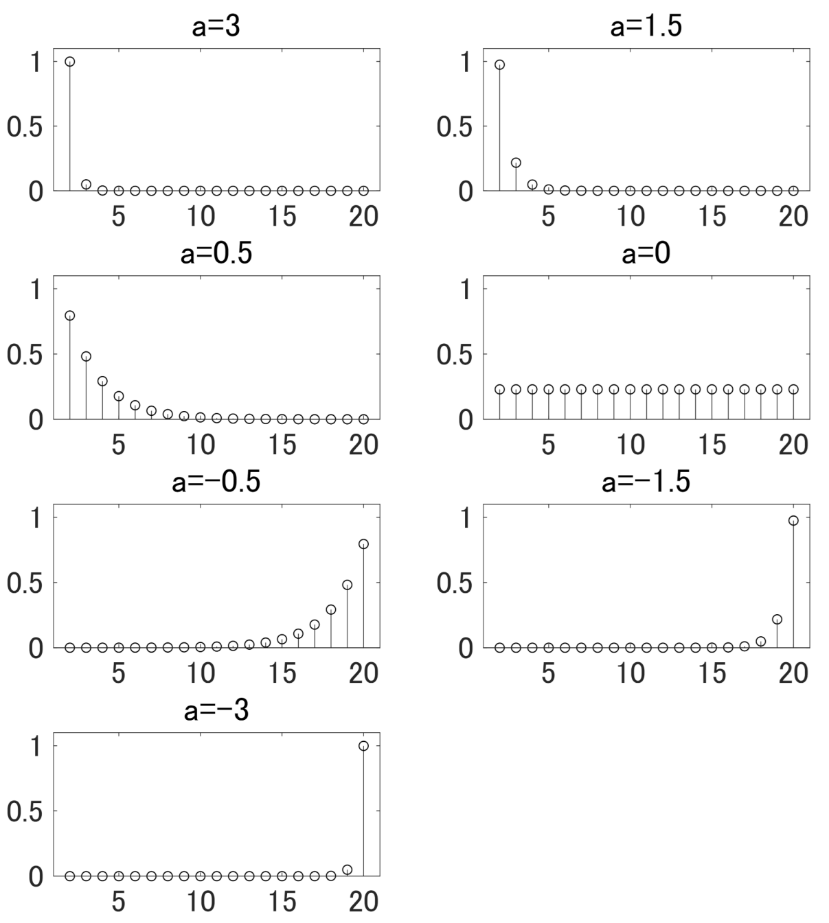
Figure 2 illustrates the results in Lemma 4. It plots for and .
Let
where . Here, is a real number, and for are defined in (44). Recall that is a basis of n-dimensional Euclidean space, and any vector in the space can be represented uniquely as a linear combination of . In addition, we note that if for , then . See (10).
Given the results presented above on and the definition of , we have the following results.
Proposition 4.
(i) c can be represented as
(ii) satisfies the following inequalities:
(iii) depends on a in (44) as
Proof.
See the Appendix A.12. □
- (i)
- Recall that (resp. ) denotes the minimum (resp. maximum) of the graph Laplacian eigenvalues, , and is the average of them. In addition, from (7), it follows that
- (ii)
- Lemma 4 and Proposition 4 imply that
- (a)
- as a increases from 0 to ∞, spatially smoother graph Laplacian eigenvectors become more dominant, and accordingly becomes spatially smoother;
- (b)
- as a decreases from 0 to , spatially less smooth graph Laplacian eigenvectors become more dominant, and accordingly becomes less spatially smoother; and
- (c)
- if a equals 0, then all graph Laplacian eigenvectors contribute to equally.
Then, we have the following results.
Proposition 5.
(ii) satisfies the following inequalities:
(iii) depends on a in (44) as
Proof.
See the Appendix A.13. □
Remark 8.
By combining Lemma 4 and Proposition 5, it follows that (i) as a increases from 0 to ∞, spatially smoother graph Laplacian eigenvectors become more dominant, and accordingly the corresponding Geary’s c tends to , which is its lower bound; (ii) as a decreases from 0 to , spatially less smooth graph Laplacian eigenvectors become more dominant, and accordingly the corresponding Geary’s c tends to , which is its upper bound; and (iii) if a equals 0, then all graph Laplacian eigenvectors contribute to equally, and the corresponding Geary’s c equals 1.
Let us illustrate Propositions 4 and 5 by specifying . We consider three ’s. The first one is in (2) with , , , and . As stated, is a non-negative, symmetric, hollow, and nonzero matrix. The second one is
where . This matrix is the adjacency matrix of a path graph such that and . See Figure A1, which depicts where . Observe that it is a non-negative, symmetric, hollow, and nonzero matrix. Some remarks on are provided in the Appendix A.14. The third one is shown in heatmap style in Figure A2. As shown in the figure, is also a nonnegative, symmetric, hollow, and nonzero matrix.
Table 1 tabulates the results. LB and UB, respectively, represent lower bound and upper bound of (resp. ) given by (50) (resp. (56)). From the table, we can confirm that these results clearly illustrate Propositions 4 and 5. That is to say, for all ’s, we can observe that as a increases from 0 to 3 (resp. decreases from 0 to ), becomes spatially smoother (resp. less smoother), and Geary’s c tends to (resp. ).
Remark 9.
(i) If , then equals . Thus, if , then it follows that . (ii) If , then equals . Thus, if , then it follows that . (iii) If , then equals . Thus, if , then it follows that .
5. Concluding Remarks
Herein, we have provided a new perspective on Geary’s c. We reconsidered it using concepts from spectral graph theory/linear algebraic graph theory.
First, we demonstrated three types of representations for it. The first is expressions based on graph Laplacian (Proposition 1), the second is expressions based on graph Fourier transform (Proposition 2), and the third is an expression based on Pearson’s correlation coefficient (Proposition 3).
Second, we illustrated that the spatial autocorrelation measured by Geary’s c is positive (resp. negative) if spatially smoother (resp. less smooth) graph Laplacian eigenvectors are dominant (Propositions 4 and 5 and Table 1).
In closing, based on our analysis, we provide a recommendation for applied studies: For detecting spatial autocorrelation, in addition to calculating Geary’s c, plotting , which is the squared Pearson’s correlation coefficient between and , for is valuable (see Section 3.4 for a related discussion). This is because
it provides more detailed information on spatial autocorrelation measured by Geary’s c. Its usefulness is similar to frequency domain analysis of univariate time series.
Funding
This research was funded by Japan Society for the Promotion of Science, grant number 20K20759.
Institutional Review Board Statement
Not applicable.
Informed Consent Statement
Not applicable.
Acknowledgments
We are grateful to Qu Feng, Kazuhiko Hayakawa, Peter C. B. Phillips, Takashi Yamagata, and two anonymous referees for their valuable suggestions and comments. We also thank the participants of the online seminars/conferences hosted by Hiroshima University, Nanyang Technological University, Singapore Management University, and University of Tokyo. The usual caveat applies.
Conflicts of Interest
The authors declare no conflict of interest.
Appendix A
Appendix A.1. The Case in Which λ2 = ⋯ = λn
Lemma A1.
If , then Geary’s c equals one for any .
Proof.
Given , we have . Then, from (30), it follows that
□
Example A1.
Consider the complete graph with n vertices whose equals . Then, in this case, equals
As the eigenvalues of are 0 with multiplicity 1 and 1 with multiplicity , the eigenvalues of are 0 with multiplicity 1 and n with multiplicity . Given that Ω equals , Geary’s c equals
Appendix A.2. Proof of (11)
Given and , we have
which leads to
Here, we note that we may prove (11) alternatively by combining
and .
Appendix A.3. Proof of (14)
can be decomposed as follows:
Given (a) , (b) , and (c) , we have
In addition, we have
and, given that for , it follows that
Finally, substituting (A3)–(A5) into (A2) yields
Appendix A.4. Proof of Lemma 1
Let . From (14), it follows that
Given (a) if , (b) for , and (c) for ,
it follows that
By substituting (A7) into (A6), we obtain . Next, given that , we have
Given these results, we have
Appendix A.5. Proof of Proposition 1
Appendix A.6. Proof of Proposition 2
Most results have already been proved, and we only have to prove that for , , and (33). (i) Given and for , we have for . (ii) Given and , we have , which leads to
(iii) Finally, we prove (33). Given (a) , (b) , (c) , and (d) for , we have
Thus, given that is an orthogonal matrix and , it follows that
Appendix A.7. Proof of Corollary 1
Given from (7) and , we have the following inequalities:
Appendix A.8. Proof of Lemma 2
Given that for , and , it follows that
In addition, from (A8), we have for . Combining these results yields
Next, the inequalities, and , immediately follow from and .
Appendix A.9. Proof of Lemma 3
Given , , and , we have
Appendix A.10. Proof of Proposition 3
Given (a) and for and (b) , we have
which leads to
Given Lemmata 2 and 3, by substituting (A11) into (28), it follows that
Finally, from Lemma 3 and (A11), it follows that
Appendix A.11. Proof of Lemma 4
For , it follows that
Accordingly, we obtain
and for ,
Therefore, given , it follows that and for as .
Likewise, for , it follows that
Accordingly, we obtain
and for ,
Therefore, given , it follows that for and as .
Appendix A.12. Proof of Proposition 4
(i) Given from (18), , and , we have
Note that the last equality in (A12) follows from (19). (ii) Given (A12), , , , and for , we have
(iii) As shown in (45), if , then for , from which we have
Next, given Lemma 4, we have
Appendix A.13. Proof of Proposition 5
(i) Given that , we have . Accordingly, given and , we obtain
Therefore, we have
Note that the last equality follows from . Next, given Lemma 4, we have
Note that the last inequalities of (A17) follow from
Appendix A.14. Some Remarks on Wp in (58)
(i) , which denotes the graph Laplacian corresponding to , is explicitly expressed as
Recall that denotes the von Neumann ratio. (iii) The graph Fourier transform corresponding to is equivalent to the discrete cosine transform developed by Ahmed et al. [15]. Denote the spectral decomposition of by
and let . Figure A3 depicts for . We can observe that has longer wavelength than for . More precisely, the period of is for . For example, the periods of and are and , respectively. Note that in the case . For more information about and , see, e.g., von Neumann [3], Jain [22], O’Sullivan [23], Strang [14], Garcia [24], Nakatsukasa et al. [25], Strang and MacNamara [26], and Yamada [27,28].
Figure A1.
A path graph with six vertices.

Figure A2.
shown in heatmap style.
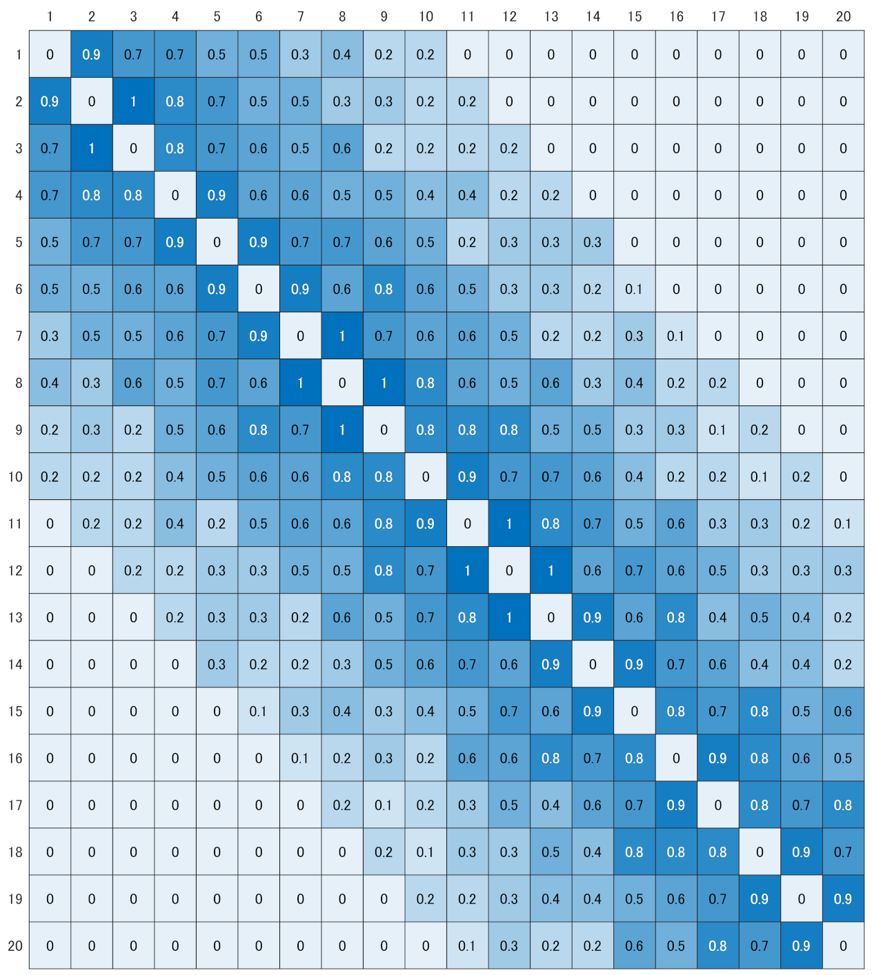
Figure A3.
The first six columns of in (A20) for .
References
- Getis, A. A history of the concept of spatial autocorrelation: A geographer’s perspective. Geogr. Anal. 2008, 40, 297–309. [Google Scholar] [CrossRef]
- Geary, R.C. The contiguity ratio and statistical mapping. Inc. Stat. 1954, 5, 115–145. [Google Scholar] [CrossRef]
- von Neumann, J. Distribution of the ratio of the mean square successive difference to the variance. Ann. Math. Stat. 1941, 12, 367–395. [Google Scholar] [CrossRef]
- de Jong, P.; Sprenger, C.; van Veen, F. On extreme values of Moran’s I and Geary’s c. Geogr. Anal. 1984, 16, 17–24. [Google Scholar] [CrossRef]
- Cliff, A.D.; Ord, J.K. The problem of spatial autocorrelation. In Studies in Regional Science; Scott, A.J., Ed.; Pion: London, UK, 1969; pp. 25–55. [Google Scholar]
- Cliff, A.D.; Ord, J.K. Spatial autocorrelation: A review of existing and new measures with applications. Econ. Geogr. 1970, 46, 269–292. [Google Scholar] [CrossRef]
- Cliff, A.D.; Ord, J.K. Spatial Autocorrelation; Pion: London, UK, 1973. [Google Scholar]
- Cliff, A.D.; Ord, J.K. Spatial Processes: Models and Applications; Pion: London, UK, 1981. [Google Scholar]
- Hammond, D.K.; Vandergheynst, P.; Gribonval, R. Wavelets on graphs via spectral graph theory. Appl. Comput. Harmon. Anal. 2011, 30, 129–150. [Google Scholar] [CrossRef] [Green Version]
- Shuman, D.I.; Narang, S.K.; Frossard, P.; Ortega, A.; Vandergheynst, P. The emerging field of signal processing on graphs: Extending high-dimensional data analysis to networks and other irregular domains. IEEE Signal Process. Mag. 2013, 30, 83–98. [Google Scholar] [CrossRef] [Green Version]
- Shuman, D.I.; Ricaud, B.; Vandergheynst, P. Vertex-frequency analysis on graphs. Appl. Comput. Harmon. Anal. 2016, 40, 260–291. [Google Scholar] [CrossRef]
- Harvey, A.C. Time Series Models, 2nd ed.; Harvester Wheatsheaf: New York, NY, USA, 1993. [Google Scholar]
- Anderson, T.W. The Statistical Analysis of Time Series; Wiley: New York, NY, USA, 1971. [Google Scholar]
- Strang, G. The discrete cosine transform. SIAM Rev. 1999, 41, 135–147. [Google Scholar] [CrossRef]
- Ahmed, N.T.; Natarajan, T.; Rao, K.R. Discrete cosine transform. IEEE Trans. Comput. 1974, 1, 90–93. [Google Scholar] [CrossRef]
- Dong, X.; Thanou, D.; Rabbat, M.; Frossard, P. Learning graphs from data: A signal representation perspective. IEEE Signal Process. Mag. 2019, 36, 44–63. [Google Scholar] [CrossRef] [Green Version]
- Ricaud, B.; Borgnat, P.; Tremblay, N.; Gonçalves, P.; Vandergheynst, P. Fourier could be a data scientist: From graph Fourier transform to signal processing on graphs. C. R. Phys. 2019, 20, 474–488. [Google Scholar] [CrossRef]
- Bapat, R.B. Graphs and Matrices, 2nd ed.; Springer: London, UK, 2014. [Google Scholar]
- Gallier, J. Spectral Theory of Unsigned and Signed Graphs. Applications to Graph Clustering: A Survey. 2016. Available online: https://arxiv.org/abs/1601.04692 (accessed on 28 September 2021).
- Lebichot, B.; Saerens, M. An experimental study of graph-based semi-supervised classification with additional node information. Knowl. Inf. Syst. 2020, 62, 4337–4371. [Google Scholar] [CrossRef]
- Dray, S. A new perspective about Moran’s coefficient: Spatial autocorrelation as a linear regression problem. Geogr. Anal. 2011, 43, 127–141. [Google Scholar] [CrossRef]
- Jain, A.K. A sinusoidal family of unitary transforms. IEEE Trans. Pattern Anal. Mach. Intell. 1979, 4, 356–365. [Google Scholar] [CrossRef] [PubMed]
- O’Sullivan, F. Discretized Laplacian smoothing by Fourier methods. J. Am. Stat. Assoc. 1991, 86, 634–642. [Google Scholar] [CrossRef]
- Garcia, D. Robust smoothing of gridded data in one and higher dimensions with missing values. Comput. Stat. Data Anal. 2010, 54, 1167–1178. [Google Scholar] [CrossRef] [Green Version]
- Nakatsukasa, Y.; Saito, N.; Woei, E. Mysteries around the graph Laplacian eigenvalue 4. Linear Algebra Its Appl. 2013, 438, 3231–3246. [Google Scholar] [CrossRef]
- Strang, G.; MacNamara, S. Functions of difference matrices are Toeplitz plus Hankel. SIAM Rev. 2014, 56, 525–546. [Google Scholar] [CrossRef] [Green Version]
- Yamada, H. A smoothing method that looks like the Hodrick–Prescott filter. Econom. Theory 2020, 36, 961–981. [Google Scholar] [CrossRef]
- Yamada, H. A pioneering study on discrete cosine transform. Commun. Stat. Theory Methods 2020, 1838547. [Google Scholar] [CrossRef]
Figure 1.
An undirected graph with four vertices.
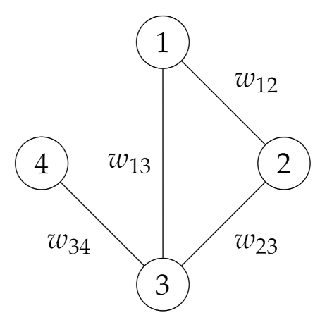
Figure 2.
in (44) for and .
Figure 2.
in (44) for and .

Publisher’s Note: MDPI stays neutral with regard to jurisdictional claims in published maps and institutional affiliations. |
© 2021 by the author. Licensee MDPI, Basel, Switzerland. This article is an open access article distributed under the terms and conditions of the Creative Commons Attribution (CC BY) license (https://creativecommons.org/licenses/by/4.0/).
Share and Cite
MDPI and ACS Style
Yamada, H. Geary’s c and Spectral Graph Theory. Mathematics 2021, 9, 2465. https://doi.org/10.3390/math9192465
AMA Style
Yamada H. Geary’s c and Spectral Graph Theory. Mathematics. 2021; 9(19):2465. https://doi.org/10.3390/math9192465
Chicago/Turabian StyleYamada, Hiroshi. 2021. "Geary’s c and Spectral Graph Theory" Mathematics 9, no. 19: 2465. https://doi.org/10.3390/math9192465
APA StyleYamada, H. (2021). Geary’s c and Spectral Graph Theory. Mathematics, 9(19), 2465. https://doi.org/10.3390/math9192465
Note that from the first issue of 2016, this journal uses article numbers instead of page numbers. See further details here.