
Analysis of the Time Fractional-Order Coupled Burgers Equations with Non-Singular Kernel Operators


Abstract
:1. Introduction
2. Basic Preliminaries
3. Methodology
3.1. Case I
3.2. Case I
4. Convergence Analysis
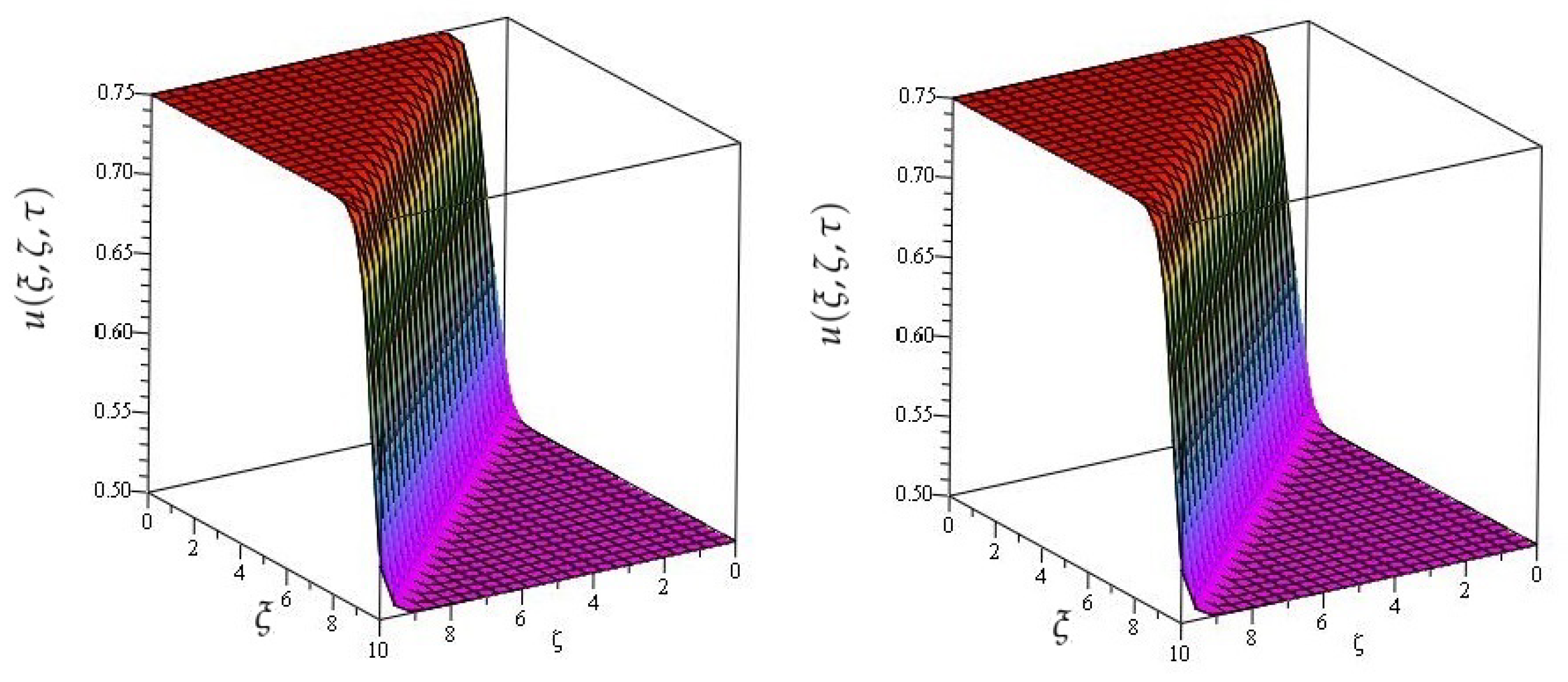
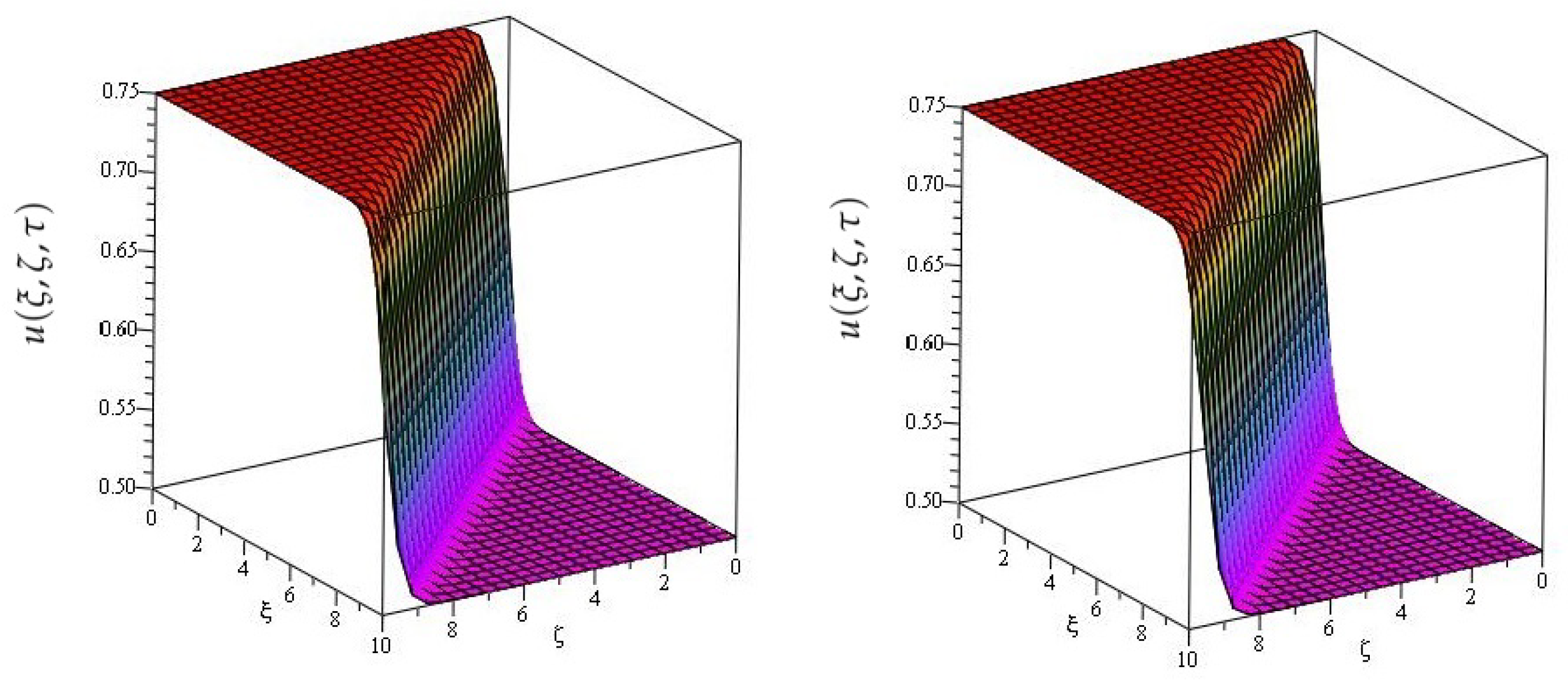
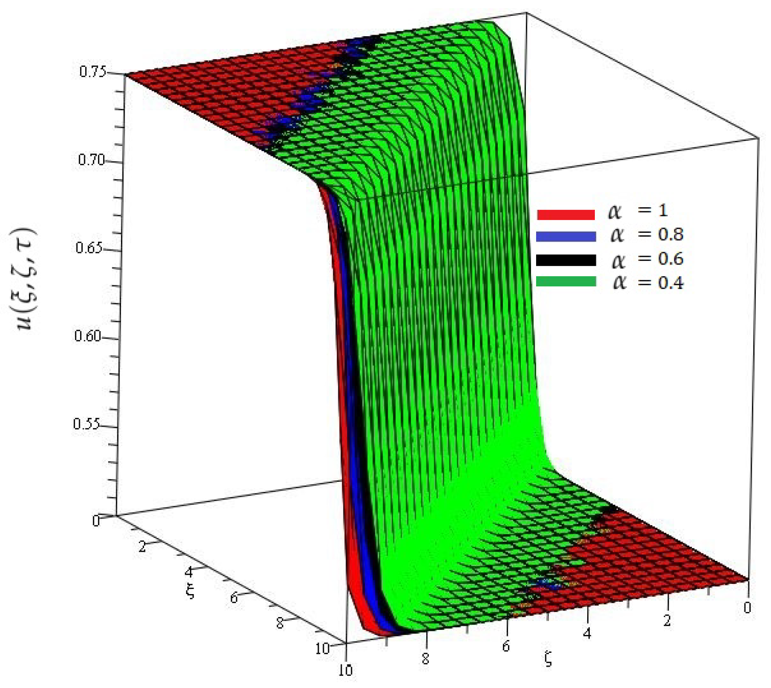
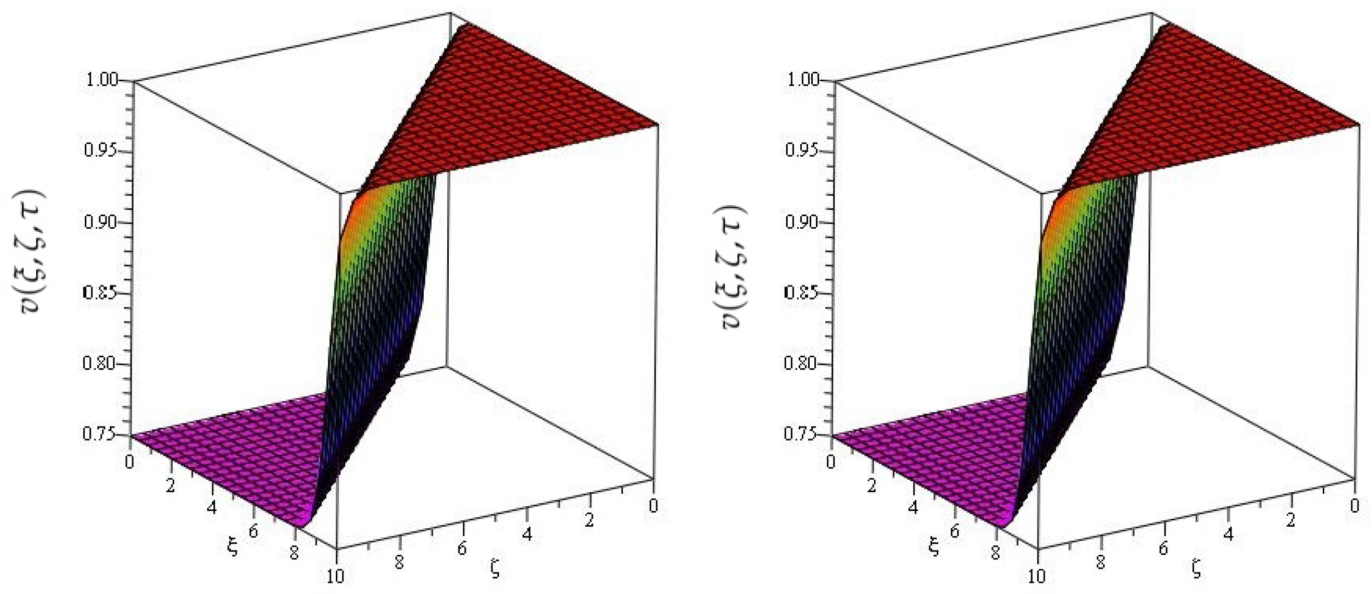
5. Numerical Examples
Numerical Results and Discussion
6. Conclusions
Author Contributions
Funding
Data Availability Statement
Conflicts of Interest
References
- Hilfer, R. Applications of Fractional Calculus in Physics; World Scientific Publishing Co., Inc.: River Edge, NJ, USA, 2000. [Google Scholar]
- Kilbas, A.A.; Srivastava, H.M.; Trujillo, J.J. Theory and Applications of Fractional Differential Equations; North Holland Mathematics Studies, Elsevier Science B.V.: Amsterdam, The Netherlands, 2006. [Google Scholar]
- Baleanu, D.; Diethelm, K.; Scalas, E.; Trujillo, J.J. Fractional Calculus, Series on Complexity, Nonlinearity and Chaos; World Scientific Publishing Co. Pte. Ltd.: Hackensack, NJ, USA, 2012; Volume 3. [Google Scholar]
- Srivastava, H.M.; Kumar, D.; Singh, J. An efficient analytical technique for fractional model of vibration equation. Appl. Math. Model. 2017, 45, 192–204. [Google Scholar] [CrossRef]
- Imtiaz, A.; Foong, O.M.; Aamina, A.; Khan, N.; Ali, F.; Khan, I. Generalized Model of Blood Flow in a Vertical Tube with Suspension of Gold Nanomaterials: Applications in the Cancer Therapy. CMC-Comput. Mater. Contin. 2020, 65, 171–192. [Google Scholar] [CrossRef]
- Aljahdaly, N.H. New application through multistage differential transform method. AIP Conf. Proc. 2020, 2293, 420025. [Google Scholar]
- Aljahdaly, N.H.; El-Tantawy, S.A. On the multistage differential transformation method for analyzing damping Duffing oscillator and its applications to plasma physics. Mathematics 2021, 9, 432. [Google Scholar] [CrossRef]
- Wu, G.C.; Baleanu, D. Variational iteration method for fractional calculus-a universal approach by Laplace transform. Adv. Differ. Equations 2013, 2013, 18. [Google Scholar] [CrossRef] [Green Version]
- Khader, M.M.; Kumar, S.; Abbasbandy, S. New homotopy analysis transform method for solving the discontinued problems arising in nanotechnology. Chin. Phys. B 2013, 22, 110201. [Google Scholar] [CrossRef]
- Jleli, M.; Kumar, S.; Kumar, R.; Samet, B. Analytical approach for time fractional wave equations in the sense of Yang-Abdel-Aty-Cattani via the homotopy perturbation transform method. Alex. Eng. J. 2020, 59, 2859–2863. [Google Scholar] [CrossRef]
- Prakash, A.; Goyal, M.; Gupta, S. q-homotopy analysis method for fractional Bloch model arising in nuclear magnetic resonance via the Laplace transform. Indian J. Phys. 2020, 94, 507–520. [Google Scholar] [CrossRef]
- Sunthrayuth, P.; Shah, R.; Zidan, A.M.; Khan, S.; Kafle, J. The Analysis of Fractional-Order Navier-Stokes Model Arising in the Unsteady Flow of a Viscous Fluid via Shehu Transform. J. Funct. Spaces 2021, 2021, 1029196. [Google Scholar]
- Mirzaee, F.; Samadyar, N. On the numerical solution of stochastic quadratic integral equations via operational matrix method. Math. Methods Appl. Sci. 2018, 41, 4465–4479. [Google Scholar] [CrossRef]
- Shah, R.; Khan, H.; Baleanu, D. Fractional Whitham-Broer-Kaup equations within modified analytical approaches. Axioms 2019, 8, 125. [Google Scholar] [CrossRef] [Green Version]
- Sohail, A.; Maqbool, K.; Ellahi, R. Stability analysis for fractional-order partial differential equations by means of space spectral time Adams Bashforth Moulton method. Numer. Methods Partial. Differ. Equ. 2018, 34, 19–29. [Google Scholar] [CrossRef]
- Burgers, J.M. Hydrodynamics-Application of a model system to illustrate some points of the statistical theory of free turbulence. In Selected Papers of JM Burgers; Springer: Dordrecht, The Netherlands, 1995; pp. 390–400. [Google Scholar]
- Aksan, E.N. Quadratic B-spline finite element method for numerical solution of the Burgers equation. Appl. Math. Comput. 2006, 174, 884–896. [Google Scholar] [CrossRef]
- Kutluay, S.; Esen, A. A lumped Galerkin method for solving the Burgers equation. Int. J. Comput. Math. 2004, 81, 1433–1444. [Google Scholar] [CrossRef]
- Abbasbandy, S.; Darvishi, M.T. A numerical solution of Burgers equation by modified Adomian method. Appl. Math. Comput. 2005, 163, 1265–1272. [Google Scholar] [CrossRef]
- Zuo, J.-M.; Zhang, Y.-M.; Abd AL-Hussein, W.R.; Mahmood, A.; Shamran, S.N.K. Exact solutions of the two-dimensional Burgers equation. J. Phys. A Math. Gen. 1999, 32, 6897–6900. [Google Scholar]
- Bateman, H. Some recent researches on the motion of fluids. Mon. Weather. Rev. 1915, 43, 163–170. [Google Scholar] [CrossRef]
- Hopf, E. The partial differential equation ut + uux = uxx. Commun. Pure Appl. Math. 1950, 3, 201–230. [Google Scholar] [CrossRef]
- Cole, J.D. On a quasi-linear parabolic equation occurring in aerodynamics. Q. Appl. Math. 1951, 9, 225–236. [Google Scholar] [CrossRef] [Green Version]
- Benton, E.R.; Platzman, G.W. A table of solutions of the one-dimensional Burgers equation. Q. Appl. Math. 1972, 30, 195–212. [Google Scholar] [CrossRef] [Green Version]
- Karpman, V.I. Non-Linear Waves in Dispersive Media: International Series of Monographs in Natural Philosophy; Elsevier: Amsterdam, The Netherlands, 2016; Volume 71. [Google Scholar]
- Rawashdeh, M.; Maitama, S. Finding exact solutions of nonlinear PDEs using the natural decomposition method. Math. Methods Appl. Sci. 2017, 40, 223–236. [Google Scholar] [CrossRef]
- Veeresha, P.; Prakasha, D.G.; Baskonus, H.M. Novel simulations to the time-fractional Fishers equation. Math. Sci. 2019, 13, 33–42. [Google Scholar] [CrossRef]
- Miller, K.S.; Ross, B. An Introduction to the Fractional Calculus and Fractional Differential Equations; A Wiley Spaces Inter Science Publication; John Wiley & Sons, Inc.: New York, NY, USA, 1993. [Google Scholar]
- Podlubny, I. Fractional Differential Equations, in Mathematics in Science and Engineering; Academic Press, Inc.: San Diego, CA, USA, 1999; p. 198. [Google Scholar]
- Diethelm, K. The Analysis of Fractional Differential Equations; Lecture Notes in Mathematics; Springer: Berlin/Heidelberg, Germany, 2010. [Google Scholar]
- Zhou, M.X.; Kanth, A.S.V.; Aruna, K.; Raghavendar, K.; Rezazadeh, H.; Mustafa Inc.; Aly, A.A. Numerical Solutions of Time Fractional Zakharov-Kuznetsov Equation via Natural Transform Decomposition Method with Nonsingular Kernel Derivatives. J. Funct. Spaces 2021, 2021, 9884027. [Google Scholar]
- Adomian, G. A new approach to nonlinear partial differential equations. J. Math. Anal. Appl. 1984, 102, 420–434. [Google Scholar] [CrossRef] [Green Version]
- Adomian, G. Solving Frontier Problems of Physics: The Decomposition Method; With a Preface by Yves Cherruault. Fundamental Theories of Physics; Kluwer Academic Publishers Group: Dordrecht, The Netherlands, 1994. [Google Scholar]
- Soliman, A.A. On the solution of two-dimensional coupled Burgers equations by variational iteration method. Chaos Solitons Fractals 2009, 40, 1146–1155. [Google Scholar] [CrossRef]


| t | ||||||
|---|---|---|---|---|---|---|
| 0.2 | 0.760060 | 0.760035 | 0.760025 | 0.760021 | 0.760021 | |
| 0.4 | 0.760148 | 0.760081 | 0.760050 | 0.760039 | 0.760040 | |
| 0.2 | 0.6 | 0.760284 | 0.760158 | 0.760095 | 0.760071 | 0.760074 |
| 0.8 | 0.760473 | 0.760278 | 0.760167 | 0.760123 | 0.760138 | |
| 1 | 0.760720 | 0.760449 | 0.760278 | 0.760205 | 0.760258 | |
| 0.2 | 0.760728 | 0.760430 | 0.760304 | 0.760258 | 0.760258 | |
| 0.4 | 0.761784 | 0.760978 | 0.760610 | 0.760477 | 0.760482 | |
| 0.4 | 0.6 | 0.763420 | 0.761915 | 0.76149 | 0.760861 | 0.760898 |
| 0.8 | 0.765698 | 0.763357 | 0.762026 | 0.761493 | 0.761673 | |
| 1 | 0.768663 | 0.765415 | 0.763362 | 0.762482 | 0.763108 | |
| 0.2 | 0.768374 | 0.765097 | 0.763645 | 0.763104 | 0.763108 | |
| 0.4 | 0.769658 | 0.761211 | 0.767177 | 0.765676 | 0.765744 | |
| 0.6 | 0.6 | 0.796654 | 0.781353 | 0.763235 | 0.760073 | 0.760522 |
| 0.8 | 0.819877 | 0.796626 | 0.782885 | 0.767192 | 0.768965 | |
| 1 | 0.849767 | 0.818099 | 0.797332 | 0.788131 | 0.793241 | |
| 0.2 | 0.821594 | 0.807747 | 0.807683 | 0.793103 | 0.793241 | |
| 0.4 | 0.848508 | 0.839515 | 0.833718 | 0.804635 | 0.805676 | |
| 0.8 | 0.6 | 0.857888 | 0.871744 | 0.867444 | 0.844863 | 0.847161 |
| 0.8 | 0.844810 | 0.899765 | 0.897914 | 0.884778 | 0.886000 | |
| 1 | 0.805199 | 0.918764 | 0.919533 | 0.925065 | 0.912839 | |
| 0.2 | 0.950038 | 0.944350 | 0.941824 | 0.923764 | 0.922839 | |
| 0.4 | 0.915159 | 0.958238 | 0.973309 | 0.958357 | 0.954325 | |
| 1 | 0.6 | 0.791894 | 0.916308 | 0.977100 | 0.978048 | 0.976759 |
| 0.8 | 0.569588 | 0.795564 | 0.931177 | 0.964956 | 0.991035 | |
| 1 | 0.238108 | 0.571732 | 0.807906 | 0.894048 | 0.909478 |
| 0.1 | 3.2300 × | 5.4246 × | 5.4246 × | |
| 0.2 | 6.9000 × | 3.4568 × | 3.4568 × | |
| 0.1 | 0.3 | 1.6200 × | 2.2468 × | 2.2468 × |
| 0.4 | 5.9700 × | 6.3267 × | 6.3267 × | |
| 0.5 | 1.8660 × | 2.1326 × | 2.1326 × | |
| 0.1 | 2.4400 × | 4.7421 × | 4.7421 × | |
| 0.2 | 8.3100 × | 3.1235 × | 3.1235 × | |
| 0.2 | 0.3 | 2.8500 × | 4.5682 × | 4.5682 × |
| 0.4 | 9.7940 × | 3.5223 × | 3.5223 × | |
| 0.5 | 3.2012 × | 2.9315 × | 2.9315 × | |
| 0.1 | 2.2981 × | 3.2245 × | 3.2245 × | |
| 0.2 | 5.4602 × | 4.2659 × | 4.2659 × | |
| 0.3 | 0.3 | 2.5432 × | 1.5348 × | 1.5348 × |
| 0.4 | 6.4229 × | 8.2374 × | 8.2374 × | |
| 0.5 | 2.8364 × | 4.1975 × | 4.1975 × | |
| 0.1 | 5.5428 × | 2.1351 × | 2.1351 × | |
| 0.2 | 2.4133 × | 2.6276 × | 2.6276 × | |
| 0.4 | 0.3 | 6.3743 × | 2.2334 × | 2.2334 × |
| 0.4 | 2.9070 × | 1.2035 × | 1.2035 × | |
| 0.5 | 6.9763 × | 2.2145 × | 2.2145 × | |
| 0.1 | 2.2529 × | 2.3223 × | 2.3223 × | |
| 0.2 | 4.9868 × | 3.2721 × | 3.2721 × | |
| 0.5 | 0.3 | 4.1932 × | 3.0767 × | 3.0767 × |
| 0.4 | 5.5568 × | 2.3742 × | 2.3742 × | |
| 0.5 | 2.4350 × | 1.3223 × | 1.3223 × |
| 0.1 | 9.0202 × | 1.3770 × | 8.6253 × | |
| 0.2 | 5.4060 × | 4.8036 × | 3.1054 × | |
| 0.1 | 0.3 | 2.7960 × | 1.6734 × | 1.1992 × |
| 0.4 | 6.5902 × | 5.8013 × | 5.5827 × | |
| 0.5 | 3.9762 × | 1.9773 × | 3.6150 × | |
| 0.1 | 3.3610 × | 2.3548 × | 2.8894 × | |
| 0.2 | 9.1810 × | 8.2143 × | 1.0171 × | |
| 0.2 | 0.3 | 1.9482 × | 2.8611 × | 3.6538 × |
| 0.4 | 9.8750 × | 9.2053 × | 1.4010 × | |
| 0.5 | 4.2127 × | 3.3727 × | 6.3855 × | |
| 0.1 | 2.3872 × | 1.2779 × | 2.3189 × | |
| 0.2 | 5.3523 × | 4.4573 × | 8.1227 × | |
| 0.3 | 0.3 | 2.5565 × | 1.5522 × | 2.8704 × |
| 0.4 | 6.3787 × | 5.3749 × | 1.0445 × | |
| 0.5 | 2.8365 × | 1.8244 × | 4.1512 × | |
| 0.1 | 5.2272 × | 4.3423 × | 1.0363 × | |
| 0.2 | 2.6215 × | 1.5145 × | 3.6229 × | |
| 0.4 | 0.3 | 6.3642 × | 5.2723 × | 1.2717 × |
| 0.4 | 2.9203 × | 1.8244 × | 4.5250 × | |
| 0.5 | 6.9958 × | 6.1751 × | 1.6814 × | |
| 0.1 | 2.2532 × | 1.1434 × | 3.3630 × | |
| 0.2 | 4.8935 × | 3.9879 × | 1.1745 × | |
| 0.5 | 0.3 | 2.4921 × | 1.3880 × | 4.1074 × |
| 0.4 | 5.8486 × | 4.7977 × | 1.4434 × | |
| 0.5 | 1.6542 × | 1.6182 × | 5.1527 × |
| 0.2 | 0.007531 | 0.003305 | 0.003056 | 0.003355 | 0.003318 | |
| 0.4 | 0.037374 | 0.010555 | 0.003583 | 0.002299 | 0.001492 | |
| 0.2 | 0.6 | 0.107634 | 0.037076 | 0.011908 | 0.005587 | 0.000671 |
| 0.8 | 0.228832 | 0.095214 | 0.035864 | 0.017981 | 0.000301 | |
| 1 | 0.409637 | 0.198269 | 0.086536 | 0.047619 | 0.000135 | |
| 0.2 | 0.010890 | 0.004952 | 0.004581 | 0.005015 | 0.004945 | |
| 0.4 | 0.054113 | 0.015998 | 0.005662 | 0.003639 | 0.002225 | |
| 0.4 | 0.6 | 0.156343 | 0.056189 | 0.019107 | 0.009354 | 0.001000 |
| 0.8 | 0.333035 | 0.144112 | 0.057207 | 0.029946 | 0.000450 | |
| 1 | 0.596925 | 0.299764 | 0.137217 | 0.078479 | 0.000202 | |
| 0.2 | 0.015625 | 0.007446 | 0.006882 | 0.007503 | 0.007368 | |
| 0.4 | 0.077841 | 0.024529 | 0.009141 | 0.005878 | 0.003318 | |
| 0.6 | 0.6 | 0.225856 | 0.086120 | 0.031439 | 0.016138 | 0.001492 |
| 0.8 | 0.482298 | 0.220396 | 0.093435 | 0.051355 | 0.000671 | |
| 1 | 0.865819 | 0.457619 | 0.222442 | 0.132987 | 0.000301 | |
| 0.2 | 0.022393 | 0.011281 | 0.010372 | 0.011236 | 0.010973 | |
| 0.4 | 0.112097 | 0.038380 | 0.015138 | 0.009711 | 0.004945 | |
| 0.8 | 0.6 | 0.326798 | 0.134623 | 0.053250 | 0.028657 | 0.002225 |
| 0.8 | 0.699653 | 0.343269 | 0.156889 | 0.090621 | 0.001000 | |
| 1 | 1.257990 | 0.710643 | 0.370200 | 0.231727 | 0.000450 | |
| 0.2 | 0.032749 | 0.017333 | 0.015694 | 0.016848 | 0.016325 | |
| 0.4 | 0.165420 | 0.062144 | 0.025783 | 0.016410 | 0.007368 | |
| 1 | 0.6 | 0.483746 | 0.217538 | 0.092962 | 0.052080 | 0.003318 |
| 0.8 | 1.036890 | 0.551429 | 0.271315 | 0.163669 | 0.001492 | |
| 1 | 1.865360 | 1.136210 | 0.633917 | 0.413380 | 0.000670 |
| 0.2 | 3.010560 | 2.998480 | 2.994809 | 2.993571 | 2.993365 | |
| 0.4 | 3.060490 | 3.019625 | 3.003995 | 2.999902 | 2.997016 | |
| 0.2 | 0.6 | 3.142602 | 3.063333 | 3.024227 | 3.011611 | 2.998659 |
| 0.8 | 3.256140 | 3.135462 | 3.063606 | 3.036047 | 2.999397 | |
| 1 | 3.400174 | 3.239966 | 3.129121 | 3.080563 | 2.999729 | |
| 0.2 | 3.015831 | 2.997739 | 2.992253 | 2.990409 | 2.990109 | |
| 0.4 | 3.090282 | 3.029146 | 3.005834 | 2.999757 | 2.995550 | |
| 0.4 | 0.6 | 3.212598 | 3.093978 | 3.035646 | 3.016907 | 2.998000 |
| 0.8 | 3.381655 | 3.200917 | 3.093647 | 3.052668 | 2.999101 | |
| 1 | 3.596061 | 3.355824 | 3.190150 | 3.117848 | 2.999596 | |
| 0.2 | 3.023772 | 2.996638 | 2.988438 | 2.985692 | 2.985263 | |
| 0.4 | 3.134729 | 3.043180 | 3.008425 | 2.999423 | 2.993365 | |
| 0.6 | 0.6 | 3.316769 | 3.139066 | 3.052084 | 3.024316 | 2.997016 |
| 0.8 | 3.568204 | 3.297118 | 3.136975 | 3.076147 | 2.998659 | |
| 1 | 3.886965 | 3.525992 | 3.278240 | 3.170692 | 2.999397 | |
| 0.2 | 3.035766 | 2.995000 | 2.982740 | 2.978658 | 2.978054 | |
| 0.4 | 3.200960 | 3.063729 | 3.011961 | 2.998675 | 2.990109 | |
| 0.8 | 0.6 | 3.471437 | 3.204907 | 3.075310 | 3.034312 | 2.995550 |
| 0.8 | 3.844671 | 3.437381 | 3.198374 | 3.108342 | 2.997999 | |
| 1 | 4.317582 | 3.773870 | 3.403204 | 3.243539 | 2.999101 | |
| 0.2 | 3.053892 | 2.992555 | 2.974226 | 2.968170 | 2.967350 | |
| 0.4 | 3.299308 | 3.093483 | 3.016524 | 2.997036 | 2.985263 | |
| 1 | 0.6 | 3.699990 | 3.299910 | 3.107172 | 3.046991 | 2.993365 |
| 0.8 | 4.252157 | 3.639306 | 3.283009 | 3.150375 | 2.997015 | |
| 1 | 4.951244 | 4.130244 | 3.575765 | 3.339528 | 2.998659 |
| 0.1 | 0.00388488 | 0.000040388 | 0.0000403885 | |
| 0.2 | 0.02058640 | 0.000643080 | 0.0006430800 | |
| 0.1 | 0.3 | 0.08300040 | 0.003204730 | 0.0032047300 |
| 0.4 | 0.19216900 | 0.009896630 | 0.0098966300 | |
| 0.5 | 0.35630400 | 0.023490500 | 0.0234905000 | |
| 0.1 | 0.00340343 | 0.000037786 | 0.0000377862 | |
| 0.2 | 0.02549380 | 0.000619573 | 0.0006195730 | |
| 0.2 | 0.3 | 0.09466810 | 0.003156030 | 0.0031560300 |
| 0.4 | 0.21124200 | 0.009911520 | 0.0099115200 | |
| 0.5 | 0.38165100 | 0.023838100 | 0.0238381000 | |
| 0.1 | 0.00290734 | 0.000030901 | 0.0000309013 | |
| 0.2 | 0.02730130 | 0.000536002 | 0.0005360020 | |
| 0.3 | 0.3 | 0.09244390 | 0.002840270 | 0.0028402700 |
| 0.4 | 0.19342500 | 0.009181990 | 0.0091819900 | |
| 0.5 | 0.33037500 | 0.022574100 | 0.0225741000 | |
| 0.1 | 0.00271456 | 0.000018180 | 0.0000181808 | |
| 0.2 | 0.02207170 | 0.000368845 | 0.0003688450 | |
| 0.4 | 0.3 | 0.06204090 | 0.002146160 | 0.0021461600 |
| 0.4 | 0.10393800 | 0.007381420 | 0.0073814200 | |
| 0.5 | 0.13365400 | 0.018959600 | 0.0189596000 | |
| 0.1 | 0.00334970 | 1.950740 × | 1.9507400 × | |
| 0.2 | 0.00408341 | 0.000093131 | 0.0000931316 | |
| 0.5 | 0.3 | 0.01675610 | 0.000951695 | 0.0009516950 |
| 0.4 | 0.10582700 | 0.004143110 | 0.0041431100 | |
| 0.5 | 0.30400000 | 0.012150100 | 0.0121501000 |
| 0.1 | 0.000409157 | 0.000080777 | 0.000080777 | |
| 0.2 | 0.00179639 | 0.00128616 | 0.00128616 | |
| 0.1 | 0.3 | 0.00575008 | 0.00640947 | 0.00640947 |
| 0.4 | 0.0154079 | 0.0197933 | 0.0197933 | |
| 0.5 | 0.0351083 | 0.046981 | 0.046981 | |
| 0.1 | 0.000358137 | 0.0000755724 | 0.0000755724 | |
| 0.2 | 0.000618968 | 0.00123915 | 0.00123915 | |
| 0.2 | 0.3 | 0.00097818 | 0.00631207 | 0.00631207 |
| 0.4 | 0.00333882 | 0.019823 | 0.019823 | |
| 0.5 | 0.0109793 | 0.0476761 | 0.0476761 | |
| 0.1 | 0.000169508 | 0.0000618027 | 0.0000618027 | |
| 0.2 | 0.00190188 | 0.001072 | 0.001072 | |
| 0.3 | 0.3 | 0.0086713 | 0.00568053 | 0.00568053 |
| 0.4 | 0.0207692 | 0.018364 | 0.018364 | |
| 0.5 | 0.0372769 | 0.0451482 | 0.0451482 | |
| 0.1 | 0.000255194 | 0.0000363616 | 0.0000363616 | |
| 0.2 | 0.00656152 | 0.00073769 | 0.00073769 | |
| 0.4 | 0.3 | 0.0259301 | 0.00429232 | 0.00429232 |
| 0.4 | 0.0634979 | 0.0147628 | 0.0147628 | |
| 0.5 | 0.122694 | 0.0379192 | 0.0379192 | |
| 0.1 | 0.00104781 | 3.90148 × | 3.90148 × | |
| 0.2 | 0.0143686 | 0.000186263 | 0.000186263 | |
| 0.5 | 0.3 | 0.0541981 | 0.00190339 | 0.00190339 |
| 0.4 | 0.132966 | 0.00828621 | 0.00828621 | |
| 0.5 | 0.261277 | 0.0243001 | 0.0243001 |
Publisher’s Note: MDPI stays neutral with regard to jurisdictional claims in published maps and institutional affiliations. |
© 2021 by the authors. Licensee MDPI, Basel, Switzerland. This article is an open access article distributed under the terms and conditions of the Creative Commons Attribution (CC BY) license (https://creativecommons.org/licenses/by/4.0/).
Share and Cite
Aljahdaly, N.H.; Agarwal, R.P.; Shah, R.; Botmart, T. Analysis of the Time Fractional-Order Coupled Burgers Equations with Non-Singular Kernel Operators. Mathematics 2021, 9, 2326. https://doi.org/10.3390/math9182326
Aljahdaly NH, Agarwal RP, Shah R, Botmart T. Analysis of the Time Fractional-Order Coupled Burgers Equations with Non-Singular Kernel Operators. Mathematics. 2021; 9(18):2326. https://doi.org/10.3390/math9182326
Chicago/Turabian StyleAljahdaly, Noufe H., Ravi P. Agarwal, Rasool Shah, and Thongchai Botmart. 2021. "Analysis of the Time Fractional-Order Coupled Burgers Equations with Non-Singular Kernel Operators" Mathematics 9, no. 18: 2326. https://doi.org/10.3390/math9182326
APA StyleAljahdaly, N. H., Agarwal, R. P., Shah, R., & Botmart, T. (2021). Analysis of the Time Fractional-Order Coupled Burgers Equations with Non-Singular Kernel Operators. Mathematics, 9(18), 2326. https://doi.org/10.3390/math9182326