Pinned Geometric Configurations in Euclidean Space and Riemannian Manifolds

Abstract

Let M be a compact d-dimensional Riemannian manifold without a boundary. Given a compact set $E\subset M$, we study the set of distances from the set E to a fixed point $x\in E$. This set is ${\Delta }_{\rho }^x\left(E\right)=\{\rho (x,y):y\in E\}$, where $\rho$ is the Riemannian metric on M. We prove that if the Hausdorff dimension of E is greater than $\frac{d+1}{2}$, then there exist many $x\in E$ such that the Lebesgue measure of ${\Delta }_{\rho }^x\left(E\right)$ is positive. This result was previously established by Peres and Schlag in the Euclidean setting. We give a simple proof of the Peres–Schlag result and generalize it to a wide range of distance type functions. Moreover, we extend our result to the setting of chains studied in our previous work and obtain a pinned estimate in this context.

1. Introduction

The celebrated Falconer distance conjecture (see e.g., [1,2]) says that if the Hausdorff dimension of a compact set $E\subset {\mathbb{R}}^d$, $d\ge 2$, is greater than $\frac{d}{2}$, then the Lebesgue measure of the distance set $\Delta \left(E\right)=\left\{\right|x-y|:x,y\in E\}$ is positive. The best known results are due to Wolff in two dimension [3] and Erdogan [4] in higher dimensions. They proved that Lebesgue measure of the distance set is positive if the Hausdorff dimension of E is greater than $\frac{d}{2}+\frac{1}{3}$. When $d=2$, Orponen ([5]) proved that in under the additional assumption that $E\subset {\mathbb{R}}^2$ is Ahlfors–David regular, if the Hausdorff dimension of E is greater than 1, then the packing dimension of the distance set $\Delta \left(E\right)=\left\{\right|x-y|:x,y\in E\}$ is 1.

An interesting variant of the Falconer distance problem is obtained by pinning the distance set. More precisely, given $x\in E$, let ${\Delta }^x\left(E\right)=\left\{\right|x-y|:y\in E\}$. Once again, the question is, how large does the Hausdorff dimension of E need to be to ensure that the Lebesgue measure of ${\Delta }^x\left(E\right)$ is positive for some x in E. Peres and Schlag ([6]) proved that the conclusion holds if the Hausdorff dimension of $E\subset {\mathbb{R}}^d$, $d\ge 2$, is greater than $\frac{d+1}{2}$. While the Peres–Schlag method, which relies on non-linear projection theory, is flexible and powerful, it is not particularly well-suited to the study of chains we undertake in this paper. Instead, we employ a rather direct approach that is suitable for a wide range of distance type functions.

For $x\in E$, E a compact subset of ${\mathbb{R}}^d$ for some $d\ge 2$, we consider

$${\Delta }_{\varphi }^x\left(E\right)=\{\varphi (x,y):y\in E\},$$

(1)

where $\varphi :{\mathbb{R}}^d\times {\mathbb{R}}^d\to \mathbb{R}$ is continuous. Further, if F is the set of points where $\varphi$ is not infinitely differentiable, then we assume that $\varphi$ is such that

$${dim}_H\left(\overline{F\cup \left\{(x,y):|{\nabla }_x\varphi (x,y)|=0\mathrm{or}|{\nabla }_y\varphi (x,y)|=0)\right\}}\right)<d+1,$$

(2)

where $\overline{A}$ denotes the closure of a set A, and ${dim}_H$ denotes the Hausdorff dimension of E. It follows then that if $\mu$ is a Frostman measure of exponent $s_E>\frac{d+1}{2}$ (see, for instance, Ref. [7] page 18 for the construction of Frostman measures), then $\mu \times \mu$ is a Frostman measure of exponent $2s_E>d+1$, and so $\varphi$ is $\mu \times \mu$-a.e. infinitely differentiable and $\mu \times \mu$-a.e. satisfies

$$|{\nabla }_x\varphi (x,y)|\ne 0\mathrm{and}|{\nabla }_y\varphi (x,y)|\ne 0.$$

(3)

Remark 1.

If, for instance, $\varphi (x,y)=|x-y|$, then the gradient is undefined on the set $\{x=y\}$. If $\varphi (x,y)=x·y$, then $|{\nabla }_x\varphi (x,y)|$ vanishes on the set $\{y=0\}$. In either example, the troublesome set has dimension at most d. Recalling that $dim\left(E\right)>\frac{d+1}{2}$, it follows that $dim(E\times E)>d+1$, and so, for each of these examples, condition (3) is violated on a set of whose dimension is strictly less than that of $E\times E$.

Remark 2.

To simplify matters, one may simply assume that we are working in a compact neighborhood of a point $(x_0,y_0)\in E\times E$ on which the function ϕ is infinitely differentiable, and on which both $|{\nabla }_x\varphi (x,y)|\ne 0$ and $|{\nabla }_y\varphi (x,y)|\ne 0$.

We also assume throughout that $\varphi$ satisfies the non-vanishing Monge–Ampere determinant assumption:

$$det\left(\begin{array}{cc}0& {\nabla }_x\varphi \\ -{\left({\nabla }_y\varphi \right)}^T& \frac{{\partial }^2\varphi }{d{x}_{i}d{y}_j}\end{array}\right)$$

(4)

does not vanish on the set $\left\{\right(x,y):\varphi (x,y)=t\}$, $t\ne 0$.

Our main results are the following.

Theorem 1.

Let E be a compact subset of ${\mathbb{R}}^d$ where $d\ge 2$, and let ${\Delta }_{\varphi }^x\left(E\right)$ be defined as in (1) above, with ϕ, as described on page 2, satisfying (2) and (4). Suppose that the Hausdorff dimension of E is greater than $\frac{d+1}{2}$. Then

$$di{m}_{\mathcal{H}}\left(\{x\in E:|{\Delta }_{\varphi }^x\left(E\right)|=0\}\right)\le d+1-di{m}_{\mathcal{H}}\left(E\right).$$

(5)

In particular, if ${\mathcal{H}}^{s_E}\left(E\right)>0$ for some $s_E>\frac{d+1}{2}$, and if μ is a Frostman measure on E of exponent $s_E$, then $|{\Delta }_{\varphi }^x\left(E\right)|>0$ for μ-a.e. $x\in E$, where ${\mathcal{H}}^{s_E}$ denotes the $s_E$-dimensional Hausdorff measure of E.

Corollary 1.

Let E be a closed subset of a compact d-dimensional, $d\ge 2$, Riemannian manifold M without a boundary and let ρ denote the Riemannian metric on M. Suppose that the Hausdorff dimension of E is greater than $\frac{d+1}{2}$. Then

$$di{m}_{\mathcal{H}}\left(\{x\in E:|{\Delta }_{\rho }^x\left(E\right)|=0\}\right)\le d+1-di{m}_{\mathcal{H}}\left(E\right).$$

(6)

In particular, if ${\mathcal{H}}^{s_E}\left(E\right)>0$ for some $s_E>\frac{d+1}{2}$, then $|{\Delta }_{\rho }^x\left(E\right)|>0$ for μ-a.e. $x\in E$, where μ is a Frostman measure of exponent $s_E>\frac{d+1}{2}$ and ${\mathcal{H}}^{s_E}$ denotes the $s_E$-dimensional Hausdorff measure of E.

Corollary 1 follows from Theorem 1 by observing that in local coordinates, the Riemannian metric $\rho$ on a compact manifold without a boundary satisfies the assumptions (3) and (4). See, for example, the Remark on the bottom of page 191 and top of page 192 in [8].

Remark 3.

As the reader will see, the method of proof of Theorem 1 is very flexible. For example, assumption on the Monge–Ampere determinant can be easily replaced by a weaker condition on the rank of the Monge–Ampere matrix. More precisely, the only thing required to obtain a non-trivial result is $L^2\left({\mathbb{R}}^d\right)\to L_{\gamma }^2\left({\mathbb{R}}^d\right)$ Sobolev bound for some $\gamma >0$ for the generalized Radon transform

$$\mathcal{R}f\left(x\right)={\int }_{\varphi (x,y)=t}f\left(y\right)\psi (x,y)d{\sigma }_{x,t}\left(y\right),$$

where ψ is a smooth cut-off function and ${\sigma }_{x,t}$ is a smooth surface measure on the set

$$\{y:\varphi (x,y)=t\}.$$

It is also important to note that in this case of the Euclidean metric, $\varphi (x,y)=|x-y|$, the only analytic input our proof uses is the fact that the operator

$$Af\left(x\right)={\int }_{S^{d-1}}f(x-y)d\sigma \left(y\right),$$

where σ is the Lebesgue measure on the sphere, maps $L^2\left({\mathbb{R}}^d\right))$ to $L_{\frac{d-1}{2}}^2\left({\mathbb{R}}^d\right)$. This is, of course, just equivalent to the well-known stationary phase estimate (see, e.g., [8])

$$|\widehat{\sigma }\left(\xi \right)|\le C{\left|\xi \right|}^{-\frac{d-1}{2}}.$$

1.1. Pinned Chains

Our methods also yield a result for pinned chains in thin subsets of Euclidean space. Let E be a compact subset of ${\mathbb{R}}^d$, $d\ge 2$, and define a k-chain in E with gaps $t=(t_1,\cdots ,t_k)$ by

$$\left\{(x^1,\cdots ,x^{k+1})\in E\times \cdots \times E:\left(\varphi (x^1,x^2),\cdots ,\varphi (x^k,x^{k+1})\right)=t\right\}.$$

Analogous to the distance set and pinned distance set, we define

$$C_{k,\varphi }\left(E\right)=\left\{\left(\varphi (x,x^2),\cdots ,\varphi (x^k,x^{k+1})\right):x,x^2,\cdots ,x^{k+1}\in E\right\},$$

(7)

and

$$C_{k,\varphi }^x\left(E\right)=\left\{\left(\varphi (x,x^2),\cdots ,\varphi (x^k,x^{k+1})\right):x^2,\cdots ,x^{k+1}\in E\right\},$$

(8)

with $\varphi$ satisfying (3) and (4).

In the special case that $\varphi$ is the Euclidean distance, it is shown in [9] that if the Hausdorff dimension of a set $E\subset {\mathbb{R}}^d$ is greater than $\frac{d+1}{2}$, then the k-dimensional Lebesgue measure

$$|C_{k,\varphi }\left(E\right)|>0.$$

(9)

Moreover, it is shown that under this assumption $C_{k,\varphi }\left(E\right)$ has non-empty interior.

We now extend this result to show that $C_{k,\varphi }^x\left(E\right)$ has positive k-dimensional Lebesgue measure for a large set of x to be quantified.

Theorem 2.

Let E be a compact subset of ${\mathbb{R}}^d$, $d\ge 2$ and let $C_{k,\varphi }^x\left(E\right)$ as in (8). Suppose that the Hausdorff dimension of E is greater than $\frac{d+1}{2}$. Then

$${dim}_{\mathcal{H}}\left(\{x\in E:\left|C_{k,\varphi }^x\left(E\right)\right|=0\}\right)\le d+1-{dim}_{\mathcal{H}}\left(E\right).$$

(10)

In particular, if ${\mathcal{H}}^{s_E}\left(E\right)>0$ for some $s_E>\frac{d+1}{2}$, then $|C_{k,\varphi }^x\left(E\right)|>0$ for μ-a.e. $x\in E$, where μ is a Frostman measure of exponent $s_E>\frac{d+1}{2}$ and ${\mathcal{H}}^{s_E}$ denotes the $s_E$-dimensional Hausdorff measure of E.

Corollary 2.

Let E be a compact subset of a compact d-dimensional, $d\ge 2$, Riemannian manifold M without a boundary and let $C_{k,\varphi }^x\left(E\right)$ be defined as in (8), where ϕ is replaced by ρ, the Riemannian metric on M. Suppose that the Hausdorff dimension of E is greater than $\frac{d+1}{2}$. Then

$${dim}_{\mathcal{H}}\left(\{x\in E:\left|C_{k,\rho }^x\left(E\right)\right|=0\}\right)\le d+1-{dim}_{\mathcal{H}}\left(E\right).$$

(11)

In particular, if ${dim}_{\mathcal{H}}\left(E\right)=s_E>\frac{d+1}{2}$, then the k-dimensional Lebesgue measure of $C_{k,\rho }\left(E\right)$, denoted by $|C_{k,\rho }^x\left(E\right)|$, is positive for μ a.e. $x\in E$, where μ is a Frostman measure of exponent $s_E>\frac{d+1}{2}$ satisfying ${\mathcal{H}}^{s_E}\left(E\right)>0$.

Corollary 2 follows from Theorem 2 in the same way Corollary 1 follows from Theorem 1.

Remark 4.

Since this paper appeared on the Arxiv, several interesting developments have taken place. Bochen Liu ([10]) proved that if the Hausdorff dimension of a compact set $E\subset {\mathbb{R}}^d$, $d\ge 2$, is greater than $\frac{d}{2}+\frac{1}{3}$, then there exists $x\in E$, such that the Lebesgue measure of ${\Delta }_x\left(E\right)$ is positive. In two dimensions this threshold was further lowered to $\frac{5}{4}$ by Guth, the first listed author of this paper, Ou and Wang in [11]. Shmerkin [12] proved that if $A\subset {\mathbb{R}}^2$ so that ${dim}_{\mathrm{H}}\left(A\right)={dim}_p\left(A\right)>1$, where ${dim}_p$ denotes the packing dimension of A, then ${dim}_{\mathrm{H}}\left({\Delta }_x\left(A\right)\right)=1$ for all x outside of a set of dimension at most 1. In the realm of chains, with the Euclidean metric, Bochen Liu lowered the dimensional threshold to $\frac{d}{2}+\frac{1}{3}$ in [13]. Once again, his method can be used to lower this threshold further to $\frac{d^2}{2d-1}$ in view of [14]. Some interesting improvements on the size of the exceptional set of x’s for which the pinned distance set ${\Delta }_x$ is small were obtained by Bochen Liu in [15]. Simon and the second listed author of this paper studied the interior of pinned distance sets corresponding to Cartesian products of Cantor sets in [16], as well as more general pinned distance sets for sets E of the critical dimension ${dim}_{\mathrm{H}}\left(E\right)=1$ in [17]. In addition see [18,19] for further results on the interior of pinned distance sets corresponding to geometric configurations.

1.2. A General Pinning Scheme

While we do not study the pinning problem in full generality in this paper, we outline the basic general mechanism in this subsection and work out a few examples. For the sake of simplicity we work with the Euclidean distance, but the arguments work equally well with functions $\varphi (x,y)$ satisfying (1) and (3). Define the edge map

$$\mathcal{E}:\{1,2,\cdots ,k+1\}\times \{1,2,\cdots ,k+1\}\to \{0,1\}$$

and let $n\left(\mathcal{E}\right)$ denote the number of non-zero values taken on by $\mathcal{E}$.

Given a compact set $E\subset {\mathbb{R}}^d$, a positive integer $k\ge 1$ and an edge map $\mathcal{E}$, we define the k-point configuration ${\mathcal{P}}_{k,\mathcal{E}}\left(E\right)$ to be the set of $n=n\left(\mathcal{E}\right)$ vectors with entries $|x^i-x^j|$ where $1\le i<j\le k+1$, $\mathcal{E}(i,j)=1$. In this way, we may naturally view ${\mathcal{P}}_{k,\mathcal{E}}\left(E\right)\subset {\mathbb{R}}^{n\left(\mathcal{E}\right)}$. For example, the chain set from the previous subsection corresponds to the edge function $\mathcal{E}(i,j)=1$, $j=i+1$, $1\le i\le k$, and 0 otherwise.

To illustrate the general pinning process, we begin with a 2-chain and pin the middle vertex. More precisely, we have

$$\mathcal{E}(1,2)=\mathcal{E}(2,3)=1$$

and the rest of the values of $\mathcal{E}(i,j)=0$. Since we are pinning the middle vertex, we are looking at the set

$${\mathcal{P}}_{2,\mathcal{E}}^x\left(E\right)=\left\{\right(|x^1-x|,|x^2-x\left|\right):x^1,x^2\in E\}.$$

Following the argument for pinned chains below in this context, and relabelling the coordinates, we see that proving that the two-dimensional Lebesgue measure of ${\mathcal{P}}_{2,\mathcal{E}}^x\left(E\right)$ is positive, we must estimate

$$\int {ϵ}^{-4}\mu \times \mu \times \mu \times \mu \times \mu \{(x^1,x^2,x^3,x^4,x^5)\in E^5:t_i-ϵ\le |x^i-x^3|\le t_i+ϵ;i\ne 3\}dt.$$

(12)

To put it another way, after relabelling the coordinates, we are led to consider ${\mathcal{P}}_{4,{\mathcal{E}}^{\prime }}\left(E\right)$, where ${\mathcal{E}}^{\prime }(i,j)=1$ if $1\le i\le 4$ and $j=5$, and 0 otherwise. This is a four vertex star with the center at $x^5$. This instantly leads to an interesting estimate because estimation of (12) leads to an $L^4$ estimate of the underlying operator (see (23) below), instead of the $L^2$ bound required to prove Theorems 1 and 2. In this case integration in t is helpful, in view of Mockenhaupt–Seeger–Sogge local smoothing estimates.

In general, in order to study the pinned version of ${\mathcal{P}}_{k,\mathcal{E}}\left(E\right)$, where the $k+1$st vertex is pinned (which we can always arrange by relabeling), we are led to consider ${\mathcal{P}}_{2k,{\mathcal{E}}^{\prime }}\left(E\right)$, where ${\mathcal{E}}^{\prime }(i,j)=\mathcal{E}(i,j)$ if $1\le i<j\le k+1$, ${\mathcal{E}}^{\prime }(k+1,k+1+j)=\mathcal{E}(j,k+1)$, ${\mathcal{E}}^{\prime }(k+1+i,k+1+j)=\mathcal{E}(i,j)$ and ${\mathcal{E}}^{\prime }(i,j)=0$ if $i<k+1$ and $j>k+1$.

A slightly more complicated situation is described in Figure 1 above. In this case $\mathcal{E}(1,2)=\mathcal{E}(2,3)=\mathcal{E}(3,4)=\mathcal{E}(1,4)=1$ and $\mathcal{E}(i,j)=0$ otherwise. Denote this configuration by ${\mathcal{P}}_{4,\mathcal{E}}$, which is precisely what is depicted on the left hand side of Figure 1. If we pin the vertex $x^4$ and apply our method, we arrive at the configuration ${\mathcal{P}}_{2k,{\mathcal{E}}^{\prime }}$ depicted on the right hand side of Figure 1.

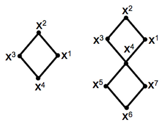
Figure 1. The pinned necklace reduces to the consideration of two necklaces sharing the pinned point.

Our method also allows us to pin two or more vertices. We shall undertake a systematic study of the pinned configurations in a subsequent paper.

2. Proof of Theorem 1

2.1. Basic Reductions

Let $\mu$ denote a Frostman measure on E of exponent $s_E>\frac{d+1}{2}$ satisfying ${\mathcal{H}}^{s_E}\left(E\right)>0$ so that

$$\mu \left(B(x,r)\right)\le C{r}^{s_E}.$$

(13)

(See, for example, [7] page 18 for the construction of such measures.)

Define the measure ${\nu }_x$ on ${\Delta }_{\varphi }^x\left(E\right)$ by the relation

$$\int f\left(t\right)d{\nu }_x\left(t\right)=\int f\left(\varphi (x,y)\right)d\mu \left(y\right).$$

(14)

Applying Cauchy–Schwarz we see that (formally)

$$1={\left(\int d{\nu }_x\left(t\right)\right)}^2\le \left|{\Delta }_{\varphi }^x\left(E\right)\right|·\int {\nu }_x^2\left(t\right)dt.$$

(15)

If we could make sense of the right hand side and show that

$$\int \int {\nu }_x^2\left(t\right)d\mu \left(x\right)dt\le C,$$

we could conclude that

$$\int {\nu }_x^2\left(t\right)dt<\infty$$

for $\mu$-a.e. $x\in E$, and plugging this into (15) would show that $|{\Delta }_{\varphi }^x\left(E\right)|>0$ for $\mu$-a.e. $x\in E$.

In order to prove the more precise estimate (5) we will show that if $\lambda$ is a compactly supported Borel measure such that

$$\lambda \left(B(x,r)\right)\le C{r}^{s_{\lambda }}$$

(16)

for some $s_{\lambda }>0$, then

$$\int \int {\nu }_x^2\left(t\right)d\lambda \left(x\right)dt\le C,$$

(17)

if

$$s_{\lambda }+di{m}_{\mathcal{H}}\left(E\right)>d+1.$$

The conclusion (5) is recovered by taking $\lambda$ to be a Frostman measure on a subset of E.

Remark 5.

The expression on the left hand side of (17), excluding the integration in t, is precisely the quantity that arises in the study of geometric hinges, first explored by the second listed author in her thesis and later studied systematically in the case $\varphi (x,y)=|x-y|$ in [9] and [20].

Remark 6.

One need not restrict attention to studying ${\Delta }_{\varphi }^x\left(E\right)$ for $x\in E$. More generally, our proof techniques extend to show that if $A\subset {\mathbb{R}}^d$ of sufficiently large dimension, then $|{\Delta }_{\varphi }^x\left(E\right)|>0$ for a.e. $x\in A.$

We now make the setup rigorous. We first address the problem set of points in (2). Let $\Psi$ be a smooth cut-off function which equals 1 on $(E\times E)\setminus N$, where N is a small open neighborhood of the set of points being measured in Equation (2). By the regularity of the measure $\mu \times \mu$ (see [21], Theorem 2.18) and by assumption (2), we can choose N so that $\mu \times \mu \left(N\right)$ is arbitrarily small. Further, assume that $\Psi$ vanishes on the closed set in Equation (2).

Next, modify the definition of ${\nu }_x$ given in (14) as follows: Set

$$\int f\left(t\right)d{\nu }_x\left(t\right)=\int f\left(\varphi (x,y)\right)\Psi (x,y)d\mu \left(y\right).$$

(18)

The plan is as follows. We will show that, for this modified measure ${\nu }_x$, the desired upper bound in (17) holds (where the expression in (17) is made formal in Lemma 1). Regarding the lower bound in Equation (15), while it no longer necessarily holds that ${\nu }_x$ is a probability measure, we observe that $\int {\nu }_x\left(t\right)>0$ is a sufficient substitute, and we now show that $\Psi$ (in (18)) can be chosen so that $\int {\nu }_x\left(t\right)>0$ for all but a $\mu$-“tiny” set of x. Indeed, let $\delta >0$ and assume that N is a small open neighborhood of the set of points being measured in Equation (2) chosen so that $\mu \times \mu \left(N\right)<\delta$. Let $N_x$ denote those points of N that have the first coordinate equal to a fixed $x\in E$. By Chebyshev’s inequality,

$$\mu \left\{x:\mu \left(N_x\right)>\frac{1}{2}\right\}<2\mu \times \mu \left(N\right)<2\delta .$$

Set $\tilde{E}=E\setminus \{x:\mu \left(N_x\right)>\frac{1}{2}\}$. Note that $\mu \left(\tilde{E}\right)>1-2\delta$ and, if $x\in \tilde{E}$, then $\mu (E\setminus N_x)\ge \frac{1}{2}$, and so, since $\Psi$ is equal to 1 on $\left(E\times E\right)\setminus N$, we have

$$\int {\nu }_x\left(t\right)=\int \Psi (x,y)d\mu \left(y\right)\ge {\int }_{E\setminus N_x}d\mu \left(y\right)>\frac{1}{2},$$

and ${\nu }_x$ is a non-zero measure. The formal argument following (14) thus yields that for $\mu$-almost every $x\in \tilde{E}$, the set ${\Delta }_x\left(E\right)$ has positive Lebesgue measure. Finally, since $\delta$ was arbitrary, this establishes that for $\mu$-almost every $x\in E$, ${\Delta }_x\left(E\right)$ has positive Lebesgue measure.

Turning to the next reduction, we will prove (17) for ${\nu }_x^{ϵ}={\nu }_x*{\psi }_{ϵ}\left(t\right)$, where $\psi$ is a smooth cut-off function, and ${\psi }_{ϵ}\left(u\right)={ϵ}^{-1}\psi (u/ϵ)$. The following Lemma provides a self-contained proof that this is sufficient. Alternatively, note that ${\nu }_x^{ϵ}$ converges to ${\nu }_x$ as measures and hence as distributions. Moreover, if $\Vert {\nu }_x^{ϵ}{\Vert }_{L^2(d\lambda \times dt)}\le C$, where C is independent of $ϵ$, then by Banach–Alaoglu we obtain that ${\nu }_x$ is absolutely continuous with respect to Lebesgue measure and has density in $L^2(d\lambda \times dt).$

Lemma 1.

Suppose that

$$\int \int {\left({\nu }_x*{\psi }_{ϵ}\left(t\right)\right)}^2\psi \left(t\right)dtd\lambda \left(x\right)\le C,$$

(19)

independently of ϵ, where ψ is a smooth cut-off function and ${\nu }_x$ is defined in (18). Then ${\nu }_x$ carries an $L^2$ density for λ-almost every $x\in E$. This would imply that, for λ-almost every x, the Lebesgue measure of ${\Delta }^x\left(E\right)$ is positive.

To prove the Lemma, let $\psi$ be a smooth cut-off function, supported in the ball of radius 2, identically equal to 1 in the ball of radius 1, centered at the origin, with $\int \psi =1$. Let ${\psi }_{ϵ}\left(u\right)={ϵ}^{-1}\psi (u/ϵ)$. Observe that by the definition of ${\nu }_x$ (see (18)),

$${\nu }_x*{\psi }_{ϵ}\left(t\right)={ϵ}^{-1}\int \psi \left(\frac{t-u}{ϵ}\right)d{\nu }_x\left(u\right)$$

$$={ϵ}^{-1}\int \psi \left(\frac{t-\varphi (x,y)}{ϵ}\right)\Psi (x,y)d\mu \left(y\right).$$

(20)

Plugging this expression into (19), it follows that

$${ϵ}^{-1}\lambda \times \mu \times \mu \{(x,y,z):|\varphi (x,y)-\varphi (x,z)|<ϵ\}\le C,$$

(21)

independently of $ϵ$.

Going back to (18), we see that

$${\widehat{\nu }}_x\left(\lambda \right)=\int e^{-2\pi i\lambda \varphi (x,y)}\Psi (x,y)d\mu \left(y\right).$$

We want to show that ${\nu }_x$ carries an $L^2$-density for $\lambda$-a.e. $x\in E$. To this end, it is enough to show that for every $ϵ>0$,

$$\int \int {|{\widehat{\nu }}_x\left(\lambda \right)|}^2\psi \left(ϵ\lambda \right)d\lambda d\mu \left(x\right)\le C,$$

independently of $ϵ$. This expression equals

$${ϵ}^{-1}\int \int \int \widehat{\psi }({ϵ}^{-1}(\varphi (x,y)-\varphi (x,z))\Psi (x,y)\Psi (x,z)d\mu \left(y\right)d\mu \left(z\right)d\mu \left(x\right)$$

and the bound follows from (21). This completes the proof of Lemma 1.

We have shown that the proof of Theorem 1 would follow if we could establish the estimate (17) with ${\nu }_x$ (defined in (18)) replaced by ${\nu }_x^{ϵ}={\nu }_x*{\psi }_{ϵ}\left(t\right)$, where $\psi$ is a smooth cut-off function. We now reduce this estimate to an operator bound. Set

$$T_{\varphi ,t}^{ϵ}f\left(x\right)=\frac{1}{ϵ}\int \psi \left(\frac{t-\varphi (x,y)}{ϵ}\right)f\left(y\right)\Psi (x,y)dy,$$

(22)

where $\varphi$ is the same as in the statement of the Theorem.

The estimate (17) would follow instantly from the operator bound

$${\left(\int {|T_{\varphi }^{ϵ}\left(f\mu \right)\left(x\right)|}^{2}d\lambda \left(x\right)\right)}^{\frac{1}{2}}\le C{\left|\right|f\left|\right|}_{L^2\left(\mu \right)}$$

(23)

under the assumption $s_{\lambda }>d+1-s_E$. Here, the constant C is uniform over t in a compact set and independent of $ϵ$, and $T_{\varphi }^{ϵ}\left(f\mu \right)\left(x\right)$ equals $T_{\varphi ,t}^{ϵ}\left(f\mu \right)\left(x\right)$ for an arbitrary t in a fixed compact set. This is where we now turn our attention.

2.2. Proof of the Operator Bound

We prove estimate (23) by showing that, for $g\in L^2\left(\lambda \right)$,

$$|<T_{\varphi }^{ϵ}f\mu ,g\lambda >|\le C{\left|\right|f\left|\right|}_{L^2\left(\mu \right)}{\left|\right|g\left|\right|}_{L^2\left(\lambda \right)}.$$

Let ${\alpha }_0\left(\xi \right)$ and $\alpha$ be smooth cut-off functions such that ${\alpha }_0$ is supported in the ball $\left\{\right|\xi |<4\}$, $\alpha$ is supported in the annulus $\{1/2\le |\xi |\le 4\}$, and ${\alpha }_0\left(\xi \right)+{\sum }_j\alpha \left(2^{-j}\xi \right)\equiv 1$.

Define $P_j{T}_{\varphi }^{ϵ}$, the classical Littlewood–Paley projection (see, for instance, [22] (pp. 241–243)), by the relation

$$\widehat{P_j{T}_{\varphi }^{ϵ}}=\widehat{T_{\varphi }^{ϵ}}·\alpha (2^{-j}·),$$

and in general, for $f\in L^2\left(dx\right)$,

$$\widehat{P_{j}f}=\widehat{f}·\alpha (2^{-j}·).$$

Let $g\in L^2\left(\lambda \right)$. Then

$$⟨T_{\varphi }^{ϵ}f\mu ,g\lambda ⟩=\sum _{j,k\ge 0}⟨T_{\varphi }^{ϵ}\left(P_{j}f\mu \right),P_{k}g\lambda )⟩.$$

(24)

This equation would probably benefit from a few words of explanation. Indeed, $T_{\varphi }^{ϵ}$ is trivially continuous $L^2\left(dx\right)\to L^2\left(dx\right)$ and, thus, in the $L^2\left(dx\right)$ sense, $T_{\varphi }^{ϵ}f\mu ={\sum }_{j\ge 0}{T}_{\varphi }^{ϵ}\left(P_{j}f\mu \right)$, if $f\mu$ were in $L^2\left(dx\right)$, and then $⟨·,·⟩$ denotes inner product in $L^2\left(dx\right)$, so the ${\sum }_{j,k\ge 0}$ can be taken out of the inner product. This is indeed what happens, except that one has to make sense of $f\mu$ and $g\lambda$, which are not in $L^2\left(dx\right)$, since the measures $\mu$ and $\lambda$ are typically singular with respect to the Lebesgue measure.

In order to do that, instead of $\mu$ and $\lambda$, consider ${\mu }_{\theta }=\mu *{\psi }_{\theta }$ and ${\lambda }_{\delta }=\lambda *{\psi }_{\delta }$ (since $ϵ$ has already been used as a parameter for regularization). Then these new measures are absolutely continuous with respect to the Lebesgue measure and we can consider $f\in L^2\left({\mu }_{\theta }\right)$ and $g\in L^2\left({\lambda }_{\delta }\right)$ which are continuous and compactly supported. Now we can run the whole argument of the proof below, and obtain (23) for the measures ${\mu }_{\theta }$ and ${\lambda }_{\delta }$. Now note that by Fubini, for any F continuous and compactly supported,

$$\int F\left(x\right)d{\mu }_{\theta }\left(x\right)=\int F\left(x\right)\left[\int \frac{1}{\theta }\psi \left(\frac{x-u}{\theta }\right)d\mu \left(u\right)\right]dx=\int \left(F*{\psi }_{\theta }\right)\left(u\right)d\mu \left(u\right).$$

(25)

Recall that if F is continuous and compactly supported, $F*{\psi }_{\theta }\to F$ uniformly. Thus, by the dominated convergence Theorem we have that, as $\theta \to 0$,

$${\parallel f\parallel }_{L^2\left({\mu }_{\theta }\right)}^2={\int \left|f\right|}^2*{\psi }_{\theta }d\mu \to {\int \left|f\right|}^{2}d\mu ={\parallel f\parallel }_{L^2\left(\mu \right)}^2.$$

(26)

On the other hand we claim that, for all x, as $\theta \to 0$, $T_{\varphi }^{ϵ}\left(f{\mu }_{\theta }\right)\left(x\right)\to T_{\varphi }^{ϵ}\left(f\mu \right)\left(x\right)$. Indeed, fix x and note that ${\Psi }_x\left(y\right)=\Psi (x,y)$ is then a continuous function in y with compact support. Then the same reasoning as (25) and (26) shows that as $\theta \to 0$,

$$\begin{array}{c}\hfill T_{\varphi }^{ϵ}\left(f{\mu }_{\theta }\right)\left(x\right)=\frac{1}{ϵ}\int \psi \left(\frac{t-\varphi (x,y)}{ϵ}\right)f\left(y\right)\Psi (x,y)d{\mu }_{\theta }\left(y\right)\\ \hfill =\frac{1}{ϵ}\int {\left[\psi \left(\frac{t-\varphi (x,·)}{ϵ}\right)f(·){\Psi }_x(·)\right]}_{\theta }\left(u\right)d\mu \left(u\right)\to T_{\varphi }^{ϵ}\left(f\mu \right)\left(x\right).\end{array}$$

As a consequence, by Fatou’s Lemma, the same reasoning as (25) and (26) for ${\lambda }_{\delta }$, and duality, we obtain (23) (for the measures $\mu$ and $\lambda$, as stated), and for f continuous and compactly supported, which, by density, yields (23) in full generality.

Returning to (24), we consider the sum over $|j-k|>K$, for a large integer K to be determined, and over $|j-k|\le K$ separately.

Lemma 2.

Let K be a positive integer. Then there exists a positive constant, dependent on K, so that

$$\sum _{|j-k|\le K}\int \widehat{T_{\varphi }^{ϵ}\left(P_{j}f\mu \right)}\left(\xi \right)\widehat{P_{k}g\lambda }\left(\xi \right)d\xi \le C{\left|\right|f\left|\right|}_{L^2\left(\mu \right)}{\left|\right|g\left|\right|}_{L^2\left(\lambda \right)}.$$

(27)

Lemma 3.

With the notation above, there exists a positive integer K such that

$$\sum _{|j-k|>K}\int \widehat{T_{\varphi }^{ϵ}\left(P_{j}f\mu \right)}\left(\xi \right)\widehat{P_{k}g\lambda }\left(\xi \right)d\xi \le C{\left|\right|f\left|\right|}_{L^2\left(\mu \right)}{\left|\right|g\left|\right|}_{L^2\left(\lambda \right)}.$$

(28)

To prove Lemma 2, we note that since the support of $P_k$ in the frequency side is contained in that of $P_{k-1}+P_k+P_{k+1}$, we can add these in front of the left hand term:

$$\begin{array}{c}\sum _{|j-k|\le K}⟨T_{\varphi }^{ϵ}\left(P_{j}f\mu \right),P_{k}g\lambda ⟩=\sum _{|j-k|\le K}⟨P_{k-1}{T}_{\varphi }^{ϵ}\left(P_{j}f\mu \right),P_{k}g\lambda ⟩+\\ \sum _{|j-k|\le K}⟨P_k{T}_{\varphi }^{ϵ}\left(P_{j}f\mu \right),P_{k}g\lambda ⟩+\sum _{|j-k|\le K}⟨P_{k+1}{T}_{\varphi }^{ϵ}\left(P_{j}f\mu \right),P_{k}g\lambda ⟩\end{array}$$

We only consider the second term above, the first and the third being similar. Then we have that

$$\begin{array}{cc}\hfill \sum _{|j-k|\le K}& ⟨P_k{T}_{\varphi }^{ϵ}\left(P_{j}f\mu \right),P_{k}g\lambda ⟩\le \hfill \\ \hfill & \sum _{|j-k|\le K}{\left(\int {|\widehat{P_{k}g\lambda }\left(\xi \right)|}^2{\left|\xi \right|}^{-d+s_{\lambda }-\eta }d\xi \right)}^{\frac{1}{2}}·{\left(\int |{\left(P_k{T}_{\varphi }^{ϵ}\left(P_{j}f\mu \right)\right)}^{\widehat{}}{|}^2{\left|\xi \right|}^{d-s_{\lambda }+\eta }d\xi \right)}^{\frac{1}{2}},\hfill \end{array}$$

(29)

for $\eta >0$ sufficiently small.

We shall need the following Lemma from [9] (Lemma 2.5). We shall give a proof below for the sake of completeness.

Lemma 4.

Let λ be a compactly supported Borel measure such that $\lambda \left(B(x,\mathbb{R})\right)\le C{\mathbb{R}}^{s_{\lambda }}$ for some $s_{\lambda }\in (0,d)$. Suppose that $\gamma >d-s_{\lambda }$. Then for $g\in L^2\left(\lambda \right)$,

$$\int {|\widehat{g\lambda }\left(\xi \right)|}^2{\left|\xi \right|}^{-\gamma }d\xi \le C^{\prime }{\left|\right|g\left|\right|}_{L^2\left(\lambda \right)}^2.$$

(30)

To prove Lemma 4, note that the left hand side of (30) can be re-written (see e.g., Proposition 8.5 in [3]) as

$$\begin{array}{cc}\hfill \int {|\widehat{g\lambda }\left(\xi \right)|}^2{\left|\xi \right|}^{-\gamma }d\xi & =c_{\gamma ,d}\int \int {|x-y|}^{\gamma -d}g\left(x\right)g\left(y\right)d\lambda \left(y\right)d\lambda \left(x\right)\hfill \\ \hfill & =c_{\gamma ,d}\int g\left(x\right)Sg\left(x\right)d\lambda \left(x\right)\hfill \\ \hfill & \le c_{\gamma ,d}·{\parallel g\parallel }_{L^2\left(\lambda \right)}·{\parallel Sg\parallel }_{L^2\left(\lambda \right)}\hfill \end{array}$$

where $Sg\left(x\right)={\int |x-y|}^{\gamma -d}g\left(y\right)d\lambda \left(y\right).$ We apply Schur’s test (see Lemma 7.5 in [3]) to verify that there exists a constant $c>0$ so that if $s_{\lambda }>d-\gamma$, then

$${\parallel Sg\parallel }_{L^2\left(\lambda \right)}\le c{\parallel g\parallel }_{L^2\left(\lambda \right)}.$$

To complete the proof of Lemma 4, we need only verify that Schur’s test applies. Observe that

$${\int |x-y|}^{\gamma -d}d\lambda \left(y\right)=\int {|x-y|}^{\gamma -d}d\lambda \left(x\right),$$

and assuming without loss of generality that the diameter of the support of $\lambda$ is at most 1,

$$\begin{array}{cc}\hfill {\int |x-y|}^{\gamma -d}d\lambda \left(y\right)& =\sum _{j\ge 0}{\int }_{\left\{2^{-(j+1)}\le |x-y|\le 2^{-j}\right\}}{|x-y|}^{\gamma -d}d\lambda \left(y\right)\hfill \\ \hfill & \le c^{\prime }\sum _{j\ge 0}{2}^{j(d-\gamma )}\lambda \left(B(x,2^{-j})\right).\hfill \end{array}$$

We recall that $\lambda \left(B(x,2^{-j})\right)\le C{2}^{-j{s}_{\lambda }}$ and conclude that the quantity above is bounded above when $s_{\lambda }>d-\gamma$. This completes the proof of Lemma 4.

Applying Lemma 4 shows that the first term on the right hand side in (29) is uniformly bounded. To handle the second term, we shall need the following classical result similar to the results obtained in [23] where the notion of rotational curvature is explicitly introduced, as well as Corollary 6.2.3 on page 173 in [8]. Since the result is not precisely covered by these references, we sketch the proof of Theorem 3 in the Appendix A below.

Theorem 3.

Let $T_{\varphi }^{ϵ}$ be defined as above with ϕ satisfying assumptions (3) and (4). Then

$$T_{\varphi }^{ϵ}:L^2\left({\mathbb{R}}^d\right)\to L_{\frac{d-1}{2}}^2\left({\mathbb{R}}^d\right)with\mathit{constants}\mathit{independent}\mathit{of}ϵ,$$

where $L_{\gamma }^2\left({\mathbb{R}}^d\right)$ denotes the Sobolev space of function with γ (generalized) derivatives in $L^2\left({\mathbb{R}}^d\right)$.

The presence of $P_k$ implies there exist constants $0<c\le C$ such that the square of the second term in the summand of (29) is bounded by

$$\int {|{\left(P_k{T}_{\varphi }^{ϵ}\left(P_{j}f\mu \right)\right)}^{\widehat{}}\left(\xi \right)|}^2{\left|\xi \right|}^{d-s_{\lambda }+\eta }d\xi \le C{2}^{k(d-s_{\lambda }+\eta )}{\int }_{c{2}^j\le \left|\xi \right|\le C{2}^j}{|{\left(T_{\varphi }^{ϵ}\left(P_{j}f\mu \right)\right)}^{\widehat{}}\left(\xi \right)|}^{2}d\xi .$$

By Theorem 3, and recalling that $|j-k|\le K$, the right hand side is bounded by

$$C{2}^{j(d-s_{\lambda }+\eta )}·2^{-j(d-1)}\int {|\widehat{P_{j}f\mu }\left(\xi \right)|}^{2}d\xi .$$

(31)

It easily follows from Lemma 4 that

$$\int {\left|\widehat{P_{j}f\mu }\left(\xi \right)\right|}^{2}d\xi \le C{2}^{j(d-s_E+{\eta }^{\prime })}{\left|\right|f\left|\right|}_{L^2\left(\mu \right)}^2,$$

for ${\eta }^{\prime }>0$ sufficiently small.

Inserting this back into (31) we obtain

$$C{2}^{j(d-s_{\lambda }+\eta )}·2^{-j(d-1)}·2^{j(d-s_E+{\eta }^{\prime })}{\left|\right|f\left|\right|}_{L^2\left(\mu \right)}^2=C{2}^{j(d+1-s_E-s_{\lambda }+\eta +{\eta }^{\prime })}{\left|\right|f\left|\right|}_{L^2\left(\mu \right)}^2.$$

The geometric series converges precisely when $s_{\lambda }>d+1-s_E$ thus completing the proof of Lemma 2.

To complete the proof of Theorem 1, it remains to prove Lemma 3 and Lemma 4. These proofs can be found in the next two subsections.

2.3. Proof of Lemma 3

(See, for example, [24], for similar arguments). Use Fourier inversion to write

$$\begin{array}{cc}\hfill T_{\varphi }^{ϵ}\left(P_{j}f\mu \right)\left(x\right)& =\int {\Phi }_{ϵ}(\varphi (x,y)-t)P_j\left(f\mu \right)\left(y\right)\Psi (x,y)dy\hfill \\ \hfill & =\int \int \int \widehat{{\Phi }_{ϵ}}\left(s\right)\widehat{P_j\left(f\mu \right)}\left(\zeta \right)exp\left(2\pi i\left(\right(\varphi (x,y)-t)s+y·\zeta )\right)\Psi (x,y)dsd\zeta dy\hfill \end{array}$$

where ${\Phi }_{ϵ}$ is $\frac{1}{2ϵ}$ times the indicator function of the interval $[-ϵ,ϵ]$.

Recalling that ${\left(P_{j}f\mu \right)}^{\widehat{}}\left(\zeta \right)=\widehat{f\mu }\left(\zeta \right)\alpha \left(2^{-j}\zeta \right)$, we have

$${\left(T_{\varphi }^{ϵ}\left(P_{j}f\mu \right)\right)}^{\widehat{}}\left(\xi \right)=\int \int \widehat{{\Phi }_{ϵ}}\left(s\right)\widehat{f\mu }\left(\zeta \right)\alpha \left(2^{-j}\zeta \right)G(s,\xi ,\zeta )dsd\zeta ,$$

(32)

where $G(s,\xi ,\zeta )=\int \int e^{\left(2\pi i\left(\right(\varphi (x,y)-t)s+y·\zeta -x·\xi )\right)}\Psi (x,y)dxdy.$

We now give an upper bound on the modulus of G in the regime that $\left|\zeta \right|\sim 2^j$ and $\left|\xi \right|\sim 2^k$.

Lemma 5.

Suppose that $\left|\zeta \right|\sim 2^j$ and $\left|\xi \right|\sim 2^k$. Then there exists a $K>0$ so that if $|j-k|>K$, then for each positive integer M, there exists a positive constant $c_M>0$ so that

$$\left|G(s,\xi ,\zeta )\right|\le c_{M}inf\left\{{\left|s\right|}^{-M},2^{-jM},2^{-kM}\right\}.$$

We give the proof of this Lemma momentarily. Returning to the calculation above, we multiply both sides of (32) by $\alpha \left(2^{-k}\xi \right)$ to see that

$$\alpha \left(2^{-k}\xi \right){\left(T_{\varphi }^{ϵ}\left(P_{j}f\mu \right)\right)}^{\widehat{}}\left(\xi \right)=\int \int {\left({\Phi }_{ϵ}\right)}^{\widehat{}}\left(s\right)\widehat{\left(f\mu \right)}\left(\zeta \right)\alpha \left(2^{-k}\xi \right)\alpha \left(2^{-j}\zeta \right)G(s,\xi ,\zeta )dsd\zeta .$$

(33)

Inserting the estimate from Lemma 5 and integrating in s, we bound (33) above in absolute value by

$$\alpha \left(2^{-k}\xi \right)min\{2^{-j(M-1)},2^{-k(M-1)}\}\int \left|\widehat{\left(f\mu \right)}\left(\zeta \right)\right|\alpha \left(2^{-j}\zeta \right)d\zeta ,$$

where M will be taken sufficiently large momentarily.

After applying Cauchy–Schwarz, we use Lemma 4 to bound this expression above by

$$\alpha \left(2^{-k}\xi \right)min\{2^{-j(M-1)},2^{-k(M-1)}\}{2}^{j(2d-s_E+{\eta }^{\prime \prime })/2}{\parallel f\parallel }_{L^2\left(\mu \right)},$$

for ${\eta }^{\prime \prime }>0$ sufficiently small.

At last,

$$\begin{array}{cc}\hfill |<& {\left(P_k{T}_{\varphi }^{ϵ}\left(P_{j}f\mu \right)\right)}^{\widehat{}},\widehat{g\lambda }>|\lesssim \hfill \\ \hfill & \int \alpha \left(2^{-k}\xi \right)\left|\widehat{g\lambda }\left(\xi \right)\right|d\xi min\{2^{-j(M-1)},2^{-k(M-1)}\}{2}^{j(2d-s_E+{\eta }^{\prime \prime })/2}{\parallel f\parallel }_{L^2\left(\mu \right)}\hfill \\ \hfill & \lesssim min\{2^{-j(M-1)},2^{-k(M-1)}\}{2}^{j(2d-s_E+{\eta }^{\prime \prime })/2}{\parallel f\parallel }_{L^2\left(\mu \right)}{2}^{k(2d-s_{\lambda }+{\eta }^{\prime \prime \prime })}{\parallel g\parallel }_{L^2\left(\lambda \right)},\hfill \end{array}$$

for an ${\eta }^{\prime \prime \prime }>0$ sufficiently small.

Summing ${\displaystyle \sum _{j,k:|j-k|>K}}$ in the previous display yields convergence of the geometric series, for an M chosen sufficiently large, thus proving the Lemma.

2.4. Proof of Lemma 5

We prove the first inequality in the statement of the Lemma, and the second follows by taking an M sufficiently large. We first compute the critical points of the phase function for

$$G(s,\xi ,\zeta )=\int \int e^{\left(2\pi i\left(\right(\varphi (x,y)-t)s+y·\zeta -x·\xi )\right)}\Psi (x,y)dxdy.$$

(34)

The critical points occur when

$$s{\nabla }_x\varphi (x,y)-\xi =0\mathrm{and}s{\nabla }_y\varphi (x,y)+\zeta =0.$$

(35)

We may assume that there exists positive constants $0<c<C$ so that

$$c<\left|{\nabla }_x\varphi (x,y)\right|<C\mathrm{and}c<\left|{\nabla }_y\varphi (x,y)\right|<C,$$

where the lower bound follows from the non degeneracy assumption in (3) coupled with the assumption that $\Psi$ has compact support.

We argue that if $\left|\zeta \right|\sim 2^j$, $\left|\xi \right|\sim 2^k$, and j and k are sufficiently separated, then both equations in (35) cannot both simultaneously hold for $(x,y)$ in the support of $\Psi$. Let us first take care of the scenario when $s=0$. If $s=0$, then we may at least assume that either $\left|\xi \right|\ne 0$ or $\left|\zeta \right|\ne 0$, and the Lemma follows by repeated integration by parts. Assume then that $s\ne 0$.

If both equations in (35) were to hold, then it would follow that

$$\frac{\left|\xi \right|}{\left|\zeta \right|}\in \left(\frac{c}{C},\frac{C}{c}\right).$$

This is clearly false if $\left|\zeta \right|\sim 2^j$, $\left|\xi \right|\sim 2^k$, and j and k are sufficiently separated. We conclude then that there exists $K>0$ so that if $|j-k|>K$, then the integrand of G is supported away from critical points.

Assuming then that $|j-k|>K$, it follows that for each $(x,y)$ in the support of $\Psi$ that either

$$s{\nabla }_x\varphi (x,y)-\xi \ne 0\mathrm{or}s{\nabla }_y\varphi (x,y)+\zeta \ne 0.$$

(36)

Fix $(x_0,y_0)$ in the support of $\Psi$, and assume the first inequality in (36) holds. Let $l\in \left\{1,\cdots ,d\right\}$ denote the coordinate such that $|s\frac{\partial \varphi (x_0,y_0)}{\partial x_{l_j}}-{\xi }_{l_j}|$ is maximal. It follows that $|s\frac{\partial \varphi (x_0,y_0)}{\partial x_{l_j}}-{\xi }_{l_j}|\ge \frac{1}{\sqrt{d}}|s{\nabla }_x\varphi (x_0,y_0)-\xi |$.

Next, we cover the compact support of $\Psi$ by finitely many open neighborhoods ${\left\{{\mathcal{U}}_j\right\}}_{j=1}^N$ about a finite collection of points ${\left\{(x_j,y_j)\right\}}_{j=1}^N$ and obtain a finite collection of coordinates ${\left\{l_j\right\}}_{j=1}^N$, so that $|s\frac{\partial \varphi (x_j,y_j)}{\partial x_{l_j}}-{\xi }_{l_j}|$ is maximal and, for each $(x,y)\in {\mathcal{U}}_j$, $|s\frac{\partial \varphi (x,y)}{\partial x_{l_j}}-{\xi }_{l_j}|\ge \frac{1}{d}|s{\nabla }_x\varphi (x_j,y_j)-\xi |$. In the case that the second equation in (36) holds for some $j\in \{1,\cdots ,N\}$, we choose the neighborhood ${\mathcal{U}}_j$ and coordinate $l_j$ in an analogous way.

Next, choose a partition of unity, ${\left\{{\Psi }_j\right\}}_{j=1}^N$, subordinate to the open cover ${\left\{{\mathcal{U}}_j\right\}}_{j=1}^N$ so that $\Psi ={\sum }_{j=1}^N{\Psi }_j$. Now, we can write

$$G(s,\xi ,\zeta )=\sum _{j=1}^N{G}_j(s,\xi ,\zeta ),$$

(37)

where

$$G_j(s,\xi ,\zeta )=\int \int e^{\left(2\pi i\left(\right(\varphi (x,y)-t)s+y·\zeta -x·\xi )\right)}{\Psi }_j(x,y)dxdy.$$

For $j\in \{1,\cdots ,N\}$ fixed, we see that $e^{\left(2\pi i\left(\right(\varphi (x,y)-t)s-x·\xi )\right)}$ is an eigenvector of the differential operator

$$\frac{1}{2\pi i(s\frac{\partial \varphi (x,y)}{\partial x_{l_j}}-{\xi }_{l_j})}\frac{\partial }{\partial x_{l_j}}.$$

(38)

Integrating by parts M times, we conclude that

$$|G_j(s,\xi ,\zeta )|\le c_M\underset{(x,y)}{sup}{\left|s\frac{\partial \varphi (x,y)}{\partial x_{l_j}}-{\xi }_{l_j}\right|}^{-M}.$$

We interpret this estimate in three separate cases: $\left\{\left|\xi \right|\le \frac{c}{2}\left|s\right|\right\}$, $\left\{2\left|s\right|C\le \left|\xi \right|\right\}$, and $\left\{2\left|s\right|C>\left|\xi \right|>\frac{c}{2}\left|s\right|\right\}$.

If $\left|\xi \right|\le \frac{c}{2}\left|s\right|$, then

$$\left|s\frac{\partial \varphi (x,y)}{\partial x_{l_j}}-{\xi }_{l_j}\right|\ge \frac{1}{d}\left|s{\nabla }_x\varphi (x_j,y_j)-\xi \right|\ge \frac{1}{d}\left(\left|s{\nabla }_x\varphi (x_j,y_j)\right|-\left|\xi \right|\right)\ge \frac{c}{2d}\left|s\right|.$$

Similarly, if $2\left|s\right|C\le \left|\xi \right|$, then

$$\left|s\frac{\partial \varphi (x,y)}{\partial x_{l_j}}-{\xi }_{l_j}\right|\ge \frac{\left|\xi \right|}{2d}.$$

In either of the first two cases, if $\left|\xi \right|\sim 2^k$,

$$|G_j(s,\xi ,\zeta )|\le C_M{inf\left\{\right|s|}^{-M},2^{-kM}\},$$

which in turn is $\le C_M{inf\left\{\right|s|}^{-M},2^{-jM},2^{-kM}\}$ if $\left|\zeta \right|\sim 2^j\le C\left|s\right|$.

In the case that $\left|\zeta \right|\sim 2^j>C\left|s\right|$, then the second inequality in (36) holds (otherwise $\frac{\left|\zeta \right|}{\left|s\right|}\in [c,C]$), and we can repeat the argument above to conclude that in this case,

$$|G_j(s,\xi ,\zeta )|\le C_M{inf\left\{\right|s|}^{-M},2^{-jM},2^{-kM}\}.$$

Now, consider the case when $\left\{2\right|s|C>|\xi |>\frac{c}{2}|s\left|\right\}$. In this regime, we claim that the second equality in (35) cannot hold. Indeed, if the second equality in (35) held, then $\left\{\right|s|C\ge |\zeta |\ge c|s\left|\right\}$. However, then note that if $|j-k|>K$, $\left|\zeta \right|\sim 2^j$, and $\left|\xi \right|\sim 2^k$, then both $\left\{2\right|s|C>|\xi |>\frac{c}{2}|s\left|\right\}$ and $\left\{\right|s|C>|\zeta |>c|s\left|\right\}$ cannot both simultaneously hold.

Thus, when we can repeat the argument above (for the second inequality in (36)), and we are only left with the case that both $\left\{2\right|s|C>|\xi |>\frac{c}{2}|s\left|\right\}$ and $\left\{2\right|s|C>|\zeta |>\frac{c}{2}|s\left|\right\}$ hold. But again, if $|j-k|>K$, $\left|\zeta \right|\sim 2^j$, and $\left|\xi \right|\sim 2^k$, then both $\left\{2\right|s|C>|\xi |>\frac{c}{2}|s\left|\right\}$ and $\left\{2\right|s|C>|\zeta |>\frac{c}{2}|s\left|\right\}$ cannot both simultaneously hold.

In all cases, we see that if $|j-k|>K$, $\left|\zeta \right|\sim 2^j$, and $\left|\xi \right|\sim 2^k$, then

$$|G_j(s,\xi ,\zeta )|\le C_M{inf\left\{\right|s|}^{-M},2^{-jM},2^{-kM}\}.$$

Recalling the $G(s,\xi ,\zeta )$ is a finite sum of such terms (see (37)), the proof of the Lemma 5 is complete.

3. Proof of Theorem 2

As before, let $\mu$ be a Frostman measure supported on E. Recall that this means that

$$\mu \left(B(x,r)\right)\le C{r}^{s_E}$$

(39)

for $s_E<di{m}_{\mathcal{H}}\left(E\right)$ and we can make $s_E$ as close to $di{m}_{\mathcal{H}}\left(E\right)$ as we want.

Let $C_{k,\varphi }^x\left(E\right)$ as in (8), and define the measure ${\nu }_x^{\left(k\right)}$ on $C_{k,\varphi }^x\left(E\right)$ by the relation

$${\int }_{{\mathbb{R}}^k}f\left(t\right)d{\nu }_x^{\left(k\right)}\left(t\right)=\int f\left(\varphi (x,x^2),\varphi (x^2,x^3),\cdots ,\varphi (x^k,x^{k+1})\right)d\mu \left(x^2\right)\cdots d\mu \left(x^{k+1}\right).$$

(40)

Applying Cauchy–Schwarz we see that (formally)

$$1={\left(\int d{\nu }_x^{\left(k\right)}\left(t\right)\right)}^2\le \left|C_{k,\varphi }^x\left(E\right)\right|·\int {\left({\nu }_x^{\left(k\right)}\left(t\right)\right)}^{2}dt.$$

(41)

As in the proof of Theorem 1, the strategy is to establish the bound

$$\int \int {\left({\nu }_x^{\left(k\right)}\left(t\right)\right)}^{2}d\mu \left(x\right)dt\le C,$$

and conclude that

$$\int {\left({\nu }_x^{\left(k\right)}\left(t\right)\right)}^{2}dt<\infty$$

for $\mu$-a.e. $x\in E$. Plugging this into (41) shows that $|{\Delta }_{\varphi }^x\left(E\right)|>0$ for $\mu$-a.e. $x\in E$.

In order to prove the more precise estimate (10) we will show that if $\lambda$ is a compactly supported Borel measure such that

$$\lambda \left(B(x,r)\right)\le C{r}^{s_{\lambda }}$$

(42)

for some $s_{\lambda }>0$, then

$$\int \int {\left({\nu }_x^{\left(k\right)}\left(t\right)\right)}^{2}d\lambda \left(x\right)dt\le C$$

(43)

if

$$s_{\lambda }+di{m}_{\mathcal{H}}\left(E\right)>d+1.$$

The conclusion (10) is recovered by taking $\lambda$ to be a Frostman measure on a subset of E.

We prove (43) by following the same basic reductions found in the proof of Theorem 1. Begin by more carefully defining the measure ${\nu }_x^k$ in (40) by introducing a product of smooth cut-off functions which avoid the problem set for the function $\varphi (x,y)$ (this is done in an analogous way to that in (18) and the following discussion). Next, let $\psi :{\mathbb{R}}^k\to {\mathbb{R}}^{+}$ be a smooth cut-off function, supported in the ball of radius 2 and identically equal to 1 in the ball of radius 1 centered at the origin, with $\int \psi =1$. Let ${\psi }_{ϵ}\left(u\right)={ϵ}^{-k}\psi (u/ϵ)$. Then by the definition of the measure ${\nu }_x^{\left(k\right)}$ given in (40),

$$\begin{array}{cc}\hfill {\nu }_x^{\left(k\right)}*{\psi }_{ϵ}\left(t\right)& ={ϵ}^{-k}\int \psi \left(\frac{t-u}{ϵ}\right)d{\nu }_x^{\left(k\right)}\left(u\right)\hfill \\ \hfill & ={ϵ}^{-k}\int \psi \left(\frac{t-\left(\varphi (x,x^2),\cdots ,\varphi (x^k,x^{k+1})\right)}{ϵ}\right)d\mu \left(x^2\right)\cdots d\mu \left(x^{k+1}\right).\hfill \end{array}$$

Let $\beta$ be a smooth cut-off function. Since the integration in t is compact owing to the compactness of E, we can throw $\beta$ in for free. Squaring and integrating with respect to $d\lambda \left(x\right)$, we obtain

$$\int \int {\left|\frac{1}{{ϵ}^k}\int \psi \left(\frac{t-\left(\varphi (x,x^2),\cdots ,\varphi (x^k,x^{k+1})\right)}{ϵ}\right)d\mu \left(x^2\right)\cdots d\mu \left(x^{k+1}\right)\right|}^{2}d\lambda \left(x\right)\beta \left(t\right)dt.$$

It follows that in order to bound

$$\int \int {\left({\nu }_x^{\left(k\right)}\left(t\right)\right)}^{2}d\lambda \left(x\right)dt$$

it suffices to set $S_{\varphi ,t}^{ϵ}$ equal the following set

$$\bigcup _{1\le i\le k}\left\{(x=x^1=y^1,x^2,\cdots ,x^{k+1},y^2,\cdots ,y^{k+1}):\left|\varphi (x^i,x^{i+1})-t_i\right|\le ϵ,\left|\varphi (y^i,y^{i+1})-t_i\right|\le ϵ\right\}$$

and show that

$$\frac{1}{{ϵ}^{2k}}\int \lambda \times \mu \times \cdots \times \mu \left\{S_{\varphi ,t}^{ϵ}\right\}\beta \left(t\right)dt\le C,$$

(44)

independently of $ϵ$.

Letting $T_{\varphi }^{ϵ}$, the operator as in (22), bounding the expression above reduces to bounding the following from above by a constant independent of t in a compact set and $ϵ>0$

$$\int {\left|T_{\varphi ,t_1}^{ϵ}\left(\left(T_{\varphi ,t_2}^{ϵ}\left(\cdots \left(T_{\varphi ,t_k}^{ϵ}\left(T_{\varphi ,t_{k+1}}^{ϵ}\left(\mu \right)·\mu \right)·\mu \right)\right)\cdots \right)·\mu \right)\right|}^{2}d\lambda \left(x\right).$$

(45)

We repeatedly apply the mapping property in (23) k times with $\lambda =\mu$ to see that this expression is bounded above when $s_{\lambda }>d+1-s_E$ and $s_E>\frac{d+1}{2}$.

References

- Falconer, K.J. On the Hausdorff dimensions of distance sets. Mathematika 1986, 32, 206–212. [Google Scholar] [CrossRef]
- Mattila, P. Geometry of Sets and Measures in Euclidean Spaces; Cambridge University Press: Cambridge, UK, 1995; Volume 44. [Google Scholar]
- Wolff, T. Lectures on Harmonic Analysis; Łaba, S.C., Ed.; University Lecture Series; American Mathematical Society: Providence, RI, USA, 2003; Volume 29. [Google Scholar]
- Erdogan, B. A bilinear Fourier extension theorem and applications to the distance set problem. IMRN 2006, 23, 2411. [Google Scholar]
- Orponen, T. On the distance sets of Ahlfors David-regular sets. Adv. Math. 2017, 307, 1029–1045. [Google Scholar] [CrossRef]
- Peres, Y.; Schlag, W. Smoothness of Projections, Bernoulli Convolutions, and the Dimension of Exceptions. Duke Math. J. 2000, 102, 193–251. [Google Scholar] [CrossRef]
- Mattila, P. Fourier Analysis and Hausdorff Dimension; Cambridge University Press: Cambridge, UK, 2015. [Google Scholar]
- Sogge, C. Fourier Integrals in Classical Analysis, 2nd ed.; Cambridge University Press: Cambridge, UK, 2017; Volume 210. [Google Scholar]
- Bennett, M.; Iosevich, A.; Taylor, K. Finite chains inside thin subsets of Rd. Anal. PDE 2016, 9, 579–614. [Google Scholar] [CrossRef][Green Version]
- Liu, B. An L2-identity and pinned distance problem. Geom. Funct. Anal. 2019, 29, 283–294. [Google Scholar] [CrossRef]
- Guth, L.; Iosevich, A.; Ou, Y.; Wang, H. On Falconer’s distance set problem in the plane. Invent. Math. 2020, 219, 779–830. [Google Scholar] [CrossRef]
- Shmerkin, P. On the Hausdorff dimension of pinned distance sets. Isr. J. Math. 2019, 230, 949–972. [Google Scholar] [CrossRef]
- Liu, B. Improvement on 2-chains inside thin subsets of Euclidean space. J. Geom. Anal. 2019, 29, 3520–3539. [Google Scholar] [CrossRef]
- Du, X.; Zhang, R. Sharp L2 estimate of Schrödinger maximal function in higher dimensions. Ann. Math. 2019, 189. [Google Scholar] [CrossRef]
- Liu, B. Hausdorff dimension of distance sets and the L2 method. Proc. Am. Math. Soc. 2020, 148, 333–341. [Google Scholar] [CrossRef]
- Simon, K.; Taylor, K. Interior of sums of planar sets and curves. Math. Proc. Camb. Philos. Soc. 2020, 168, 119–148. [Google Scholar] [CrossRef]
- Simon, K.; Taylor, K. Dimension and measure of sums of planar sets and curves. arXiv 2017, arXiv:1707.01407. [Google Scholar]
- Greenleaf, A.; Iosevich, A.; Taylor, K. On k-point configurations with nonempty interior, to appear. arXiv 2021, arXiv:2005.10796. [Google Scholar]
- Greenleaf, A.; Iosevich, A.; Taylor, K. Configuration Sets with Nonempty interior. J Geom. Anal. 2021, 31, 6662–6680. [Google Scholar] [CrossRef]
- Iosevich, A.; Krause, B.; Sawyer, E.; Taylor, K.; Uriarte-Tuero, I. Maximal operators: Scales, curvature and the fractal dimension. Anal. Math. 2019, 45, 63–86. [Google Scholar] [CrossRef]
- Rudin, W. Real and Complex Analysis, 3rd ed.; McGraw-Hill Book CO.: New York, NY, USA, 1987. [Google Scholar]
- Stein, E.M. Harmonic Analysis; Princeton University Press: Princeton, NJ, USA, 1993. [Google Scholar]
- Phong, D.; Stein, E. Hilbert integrals, singular integrals and Radon transforms I. Acta Math. 1986, 157, 99–157. [Google Scholar] [CrossRef]
- Eswarathasan, S.; Iosevich, A.; Taylor, K. Fourier integral operators, fractal sets, and the regular value theorem. Adv. Math. 2011, 228, 2385–2402. [Google Scholar] [CrossRef]
- Duistermaat, J. Fourier Integral Operators, Progress in Mathematics; Birkhäuser Boston, Inc.: Boston, MA, USA, 1996; Volume 130. [Google Scholar]
- Hormander, L. The Analysis of Linear Partial Differential Operators, III; Springer: Berlin/Heidelberg, Germany, 1994. [Google Scholar]
Publisher’s Note: MDPI stays neutral with regard to jurisdictional claims in published maps and institutional affiliations. |
© 2021 by the authors. Licensee MDPI, Basel, Switzerland. This article is an open access article distributed under the terms and conditions of the Creative Commons Attribution (CC BY) license (https://creativecommons.org/licenses/by/4.0/).