Adaptive Online Learning for the Autoregressive Integrated Moving Average Models

Abstract

This paper addresses the problem of predicting time series data using the autoregressive integrated moving average (ARIMA) model in an online manner. Existing algorithms require model selection, which is time consuming and unsuitable for the setting of online learning. Using adaptive online learning techniques, we develop algorithms for fitting ARIMA models without hyperparameters. The regret analysis and experiments on both synthetic and real-world datasets show that the performance of the proposed algorithms can be guaranteed in both theory and practice.

1. Introduction

The autoregressive integrated moving average (ARIMA) model is an important tool for time series analysis [1], and has been successfully applied to a wide range of domains including the forecasting of household electric consumption [2], scheduling in smart grids [3], finance [4], and environment protection [5]. It specifies that the values of a time series depend linearly on their previous values and error terms. In recent years, online learning (OL) methods have been applied to estimate the univariate [6,7] and multivariate [8,9] ARIMA models for their efficiency and scalability. These methods are based on the fact that any ARIMA model can be approximated by a finite dimensional autoregressive (AR) model, which can be fitted incrementally using online convex optimization algorithms. However, to guarantee accurate predictions, these methods require a proper configuration of hyperparameters, such as the diameter of the decision set, the learning rate, the order of differencing, and the lag of the AR model. Theoretically, these hyperparameters need to be set according to prior knowledge about the data generation, which is impossible to obtain. In practice, the hyperparameters are usually tuned to optimize the goodness of fit on the unseen data, which requires numerical simulation (e.g., cross-validation) on a previously collected dataset. The numerical simulation is notoriously expensive, since it requires multiple training runs for each candidate hyperparameter configuration. Furthermore, a previously collected dataset containing ground truth is needed for validation of the fitted model, which is unsuited for the online setting. Unfortunately, the expensive tuning process needs to be regularly repeated if the statistical properties of the time series change over time in an unforeseen way.

Given a new problem of predicting time series values, it appears that tuning the hyperparameters of the online algorithms can negate the benefits of the online setting. This paper addresses this problem in the online learning framework by proposing new parameter-free algorithms for learning ARIMA models, while their performance can still be guaranteed in both theory and practice. A naive attempt for this would be to directly apply parameter-free online convex optimization (PF-OCO) algorithms to the AR approximation. However, the theoretical performance of the AR approximation and the parameter-free algorithms rely on the bounded gradient vectors of the loss function, which is unreasonable for the widely used squared error with an unbounded domain.

The key contribution of this paper is the design of online learning algorithms for ARIMA models, avoiding regular and expensive hyperparameter tuning without damaging the power of the models. Our algorithms update the model incrementally with a computational complexity that is linearly related to the size of the model parameters and the number of candidate models in each iteration. To obtain a solid theoretical foundation, we first show that, for any locally Lipschitz-continuous function, ARIMA models with fixed order of differencing can be approximated using an AR model of the same order for a large enough lag. Based on this, new algorithms are proposed for learning the AR model adaptively without requiring any prior knowledge about the model parameters. For Lipschitz-continuous loss functions, we apply a new algorithm based on the adaptive follow the regularized leader (FTRL) framework [10] and show that our algorithm achieves a sublinear regret bound depending on the data sequence and the Lipschitz constant. A special treatment on the commonly used squared error is required due to its non-Lipschitz continuity. To obtain a data-dependent regret bound, we combine a polynomial regularizer [11] with the adaptive FTRL framework. Finally, to find the proper order and lag of the AR model in an online manner, multiple AR models are simultaneously maintained, and an adaptive hedge algorithm is applied to aggregate their predictions. In the previous attempts [12,13] to solve this online model selection (OMS) problem, the exponentiated gradient (EG) algorithm has been directly applied to aggregate the predictions, which not only requires tuning the learning rate, but also yields a regret bound depending on the loss incurred by the worst model. Our adaptive hedge algorithm is parameter-free and guarantees a regret bound depending on the time series sequence. Table 1 provides a comparison of the online learning algorithms applied to the learning of the ARIMA models. In addition to the theoretical analysis, we also demonstrate the performance of the proposed algorithm using both synthetic and real-world datasets.

Table 1. Algorithms for online learning of ARIMA.

Problem	Algorithm	Reference	Tuning-Free	Loss Function	Regret Dependence
OL for ARIMA	OGD	[6,7,8,9]	✗	any	largest gradient norm
OL for ARIMA	ONS	[6,7,8,9]	✗	exp-concave	largest gradient norm
PF-OCO	Coin Betting	[14,15]	✔	normalized gradient	gradient vectors
PF-OCO	FreeRex	[16]	✔	any	largest gradient norm
PF-OCO	SF-MD	[17]	✗	any	gradient vectors
PF-OCO	SOLO-FTRL	[17]	✔	any	largest gradient norm
OL for ARIMA	Algorithm 1	This Paper	✔	Lipschitz	data sequence
OL for ARIMA	Algorithm 2	This Paper	✔	squared error	data sequence
OMS for ARIMA	EG	[12,13]	✗	bounded	loss of the worst model
OMS for ARIMA	Algorithm 3	This Paper	✔	local Lipschitz	data sequence

For non-Lipschitz-continuous loss functions, the gradient norm can be unbounded. These algorithms with performance depending on the gradient norm can fail without making further assumptions on the data generation. For OGD, the learning rate and the diameter of the decision set need to be tuned in practice. ONS has an additional hyperparameter controlling the numerical stability. Applying SF-MD to ARIMA, the diameter of the model parameter has to be tuned. To obtain optimal performance, the learning rate of EG has to be tuned.

The rest of the paper is organized as follows. Section 2 reviews the existing work on the subject. The notation, learning model, and formal description of the problem are introduced in Section 3. Next, we present and analyze our algorithms in Section 4. Section 5 demonstrates the empirical performance of the proposed methods. Finally, we conclude our work with some future research directions in Section 6.

Algorithm 1 ARIMA-AdaFTRL.

Input: $L_1>0$ Initialize ${\theta }_{1,i}$ arbitrarily, ${\eta }_{1,i}=0$, $G_{i,0}=0$ for $i=1,\dots ,m$ for$t=1$ to T do   for $i=1$ to m do     $G_{i,t}=max\{G_{i,t-1},{\parallel {▿}^d{X}_{t-i}\parallel }_2\}$     ${\eta }_{i,t}={\parallel {\theta }_{i,1}\parallel }_F+\sqrt{{\sum }_{s=1}^{t-1}{\parallel g_{i,s}\parallel }_F^2+{\left(L_t{G}_{i,t}\right)}^2}$     if ${\eta }_{i,t}\ne 0$ then      ${\gamma }_{i,t}=\frac{{\theta }_{i,t}}{{\eta }_{i,t}}$     else      ${\gamma }_{i,t}=0$     end if   end for   Play ${\tilde{X}}_t\left({\gamma }_t\right)$   Observe $X_t$ and $h_t\in \partial l_t\left({\tilde{X}}_t\left({\gamma }_t\right)\right)$   $L_{t+1}=max\{L_t,{\parallel g_t\parallel }_2\}$   for $i=1$ to m do     $g_{i,t}=g_t{▿}^d{X}_{t-i}^{\top }$     ${\theta }_{i,t+1}={\theta }_{i,t}-g_{i,t}$   end for end for

Algorithm 2 ARIMA-AdaFTRL-Poly.

Input: $G_0>0$ Initialize ${\theta }_1$ arbitrarily, $G_1=max\{G_0,{\parallel {▿}^d{X}_0\parallel }_2,\dots ,{\parallel {▿}^d{X}_{-m+1}\parallel }_2\}$ for$t=1$ to T do   ${\eta }_t={\parallel {\theta }_1\parallel }_F+\sqrt{{\sum }_{s=1}^{t-1}{\parallel {▿}^d{X}_s{x}_s^{\top }\parallel }_F^2+{\left(G_t{\parallel x_t\parallel }_2\right)}^2}$   ${\lambda }_t=\sqrt{{\sum }_{s=1}^t{\parallel x_s\parallel }_2^4}$   if ${\parallel {\theta }_t\parallel }_F\ne 0$ then     Select $c\ge 0$ satisfying ${\lambda }_t{c}^3+{\eta }_{t}c={\parallel {\theta }_t\parallel }_F$     ${\gamma }_t=\frac{c{\theta }_t}{{\parallel {\theta }_t\parallel }_F}$   else     ${\gamma }_t=0$   end if   Play ${\tilde{X}}_t\left({\gamma }_t\right)$   Observe $X_t$ and $g_t={\gamma }_t{x}_t-{▿}^d{X}_t$   $G_{t+1}=max\{G_t,{\parallel {▿}^d{X}_t\parallel }_2\}$   ${\theta }_{t+1}={\theta }_t-g_t{x}_t^{\top }$ end for

Algorithm 3 ARIMA-AO-Hedge.

Input: predictor ${\mathcal{A}}_1,\dots ,{\mathcal{A}}_K$, d Initialize ${\theta }_{k,1}=0$, ${\eta }_1=0$ for $i=1,\dots ,K$ for$t=1$ to T do   Get prediction ${\tilde{X}}_t^i$ from ${\mathcal{A}}_k$ for $i=1,\dots ,K$   Set $Y_t={\sum }_{i=0}^{d-1}{▿}^i{X}_{t-1}$   Set $h_{i,t}=l(Y_t,{\tilde{X}}_t^i)$ for $i=1,\dots ,K$   if ${\eta }_1=0$ then     Set $w_{i,t}=1$ for some $i\in arg{max}_{j\in \{1,\dots ,K\}}{h}_{j,t}$   else     Set $w_{i,t}=\frac{exp\left({\eta }_t^{-1}({\theta }_{i,t}-h_{i,t})\right)}{{\sum }_{i=1}^{K}exp\left({\eta }_t^{-1}({\theta }_{i,t}-h_{i,t})\right)}$ for $i=1,\dots ,K$   end if   Predict ${\tilde{X}}_t={\sum }_{i=1}^K{w}_{i,t}{\tilde{X}}_t^i$   Observe $X_t$, update ${\mathcal{A}}_i$, and set $z_{i,t}=l(X_t,{\tilde{X}}_t^i)$ for $i=1,\dots ,K$   ${\theta }_{t+1}={\theta }_t-z_t$   ${\eta }_{t+1}=\sqrt{\frac{1}{2logK}{\sum }_{s=1}^t{\parallel h_t-z_t\parallel }_{\infty }^2}$ end for

2. Related Work

An ARIMA model can be fitted using statistical methods such as recursive least square and maximum likelihood estimation, which are not only based on strong assumptions such as the Gaussian distributed noise terms [18], linear dependencies [19], and data generated by a stationary process [20], but also require solution of non-convex optimization problems [21]. Although these assumptions can be relaxed by considering non-Gaussian noise [22,23], non-stationary processes [24], or a convex relaxation [21], the pre-trained models still cannot deal with concept drift [7]. Moreover, retraining is time consuming and memory intensive, especially for large-scale datasets. The idea of applying regret minimization techniques to autoregressive moving average (ARMA) prediction was first introduced in [6]. The authors propose online algorithms incrementally producing predictions close to the values generated by the best ARMA model. This idea was extended to $ARIMA(p,q,d)$ models in [7] by learning the $AR\left(m\right)$ model of the higher-order differencing of the time series. Further extensions to multiple time series can be found in [8,9], while the problem of predicting time series with missing data was addressed in [25].

In order to obtain accurate predictions, the lag of the AR model and the order of differencing have to be tuned, which has been well studied in the offline setting. In some textbooks [20,26,27], Akaike’s Information Criterion (AIC) and the Bayesian Information Criterion (BIC) are recommended for this task. Both require prior knowledge and strong assumptions about the variance of the noise [20], and are time and space consuming as they require numerical simulation such as cross-validation on previously collected datasets. Nevertheless, given a properly selected lag m and order d, online convex optimization techniques such as online Newton step (ONS) or online gradient descent (OGD) can be applied to fitting the model in the regret minimization framework [6,7,8,9]. However, both algorithms introduce additional hyperparameters to control the learning rate and numerical stability.

The idea of selecting hyperparameters for online time series prediction was proposed in [12,13]. Regarding the online AR predictor with different lags as experts, the authors aggregate over predictors by applying a multiplicative weights algorithm for prediction with expert advice. The proposed algorithm is not optimal for time series prediction, since the regret bound of the chosen algorithm depends on the largest loss incurred by the experts [28]. Furthermore, each individual expert still requires that the parameters are taken from a compact decision set, the diameter of which needs to be tuned in practice. A series of recent works on parameter-free online learning have provided possibilities of achieving sublinear regret without prior information on the decision set. In [14], the unconstrained online learning problem is modeled as a betting game, based on which a parameter-free algorithm is developed. The algorithm was further extended in [15], so a better regret bound can be achieved for strongly convex loss functions. However, the coin betting algorithm requires that the gradient vectors are normalized, which is unrealistic for unbounded time series and the squared error loss. In [16,17], the authors introduced parameter-free algorithms without requiring normalized gradient vectors. Unfortunately, the regret upper bounds of the proposed algorithms depend on the norm of the gradient vectors, which could be extremely large in our setting.

The main idea of the current work is based on the combination of the adaptive FTRL framework [10] and the idea of handling relative Lipschitz continuous functions [11], which makes it possible to devise an online algorithm with a data-dependent regret upper bound. To aggregate the results, an adaptive optimistic algorithm is proposed, such that the overall regret depends on the data sequence instead of the worst-case loss.

3. Preliminary and Learning Model

Let $X_t$ denote the value observed at time t of a time series. We assume that $X_t$ is taken from a finite dimensional real vector space $\mathbb{X}$ with norm $\parallel ·\parallel$. We denote by $\mathcal{L}(\mathbb{X},\mathbb{X})$ the vector space of bounded linear operators from $\mathbb{X}$ to $\mathbb{X}$ and ${\parallel \alpha \parallel }_{op}={sup}_{x\in \mathbb{X},x\ne 0}\frac{\parallel \alpha x\parallel }{\parallel x\parallel }$ the corresponding operator norm. An $AR\left(p\right)$ model is given by

$$X_t=\sum _{i=1}^p{\alpha }_i{X}_{t-i}+{ϵ}_t,$$

where ${\alpha }_i\in \mathcal{L}(\mathbb{X},\mathbb{X})$ is a linear operator and ${ϵ}_t\in \mathbb{X}$ is an error term. The $ARMA(p,q)$ model extends the $AR\left(p\right)$ model by adding a moving average (MA) component as follows:

$$X_t=\sum _{i=1}^p{\alpha }_i{X}_{t-i}+\sum _{i=1}^q{\beta }_i{ϵ}_{t-i}+{ϵ}_t,$$

where ${ϵ}_t\in \mathbb{X}$ is the error term and ${\beta }_i\in \mathcal{L}(\mathbb{X},\mathbb{X})$. We define the d-th order differencing of the time series as ${▿}^d{X}_t={▿}^{d-1}{X}_t-{▿}^{d-1}{X}_{t-1}$ for $d\ge 1$ and ${▿}^0{X}_t=X_t$. The $ARIMA(p,q,d)$ model assumes that the d-th order differencing of the time series follows an $ARMA(p,q)$ model. In this section, this general setting suffices for introducing the learning model. In the following sections, we fix the basis of $\mathbb{X}$ to obtain implementable algorithms, for which different kinds of norms and inner products for vectors and matrices are needed. We provide a table of required notation in Appendix C.

In this paper, we consider the setting of online learning, which can be described as an iterative game between a player and an adversary. In each round t of the game, the player makes a prediction ${\tilde{X}}_t$. Next, the adversary chooses some $X_t$ and reveals it to the player, who then suffers the loss $l(X_t,\widetilde{X_t})$ for some convex loss function $l:\mathbb{X}\times \mathbb{X}\to \mathbb{R}$. The ultimate goal is to design a strategy for the player to minimize the cumulative loss ${\sum }_{t=1}^{T}l(X_t,\widetilde{X_t})$ of T rounds. For simplicity, we define

$$l_t:\mathbb{X}\to \mathbb{R},X\mapsto l(X_t,X).$$

In classical textbooks about time series analysis, the signal is assumed to be generated by a model, based on which the predictions are made. In this paper, we make no assumptions on the data generation. Therefore, minimizing the cumulative loss is generally impossible. An achievable objective is to keep a possibly small regret of not having chosen some $ARIMA(p,q,d)$ model to generate the prediction ${\tilde{X}}_t$. Formally, we denote by ${\tilde{X}}_t(\alpha ,\beta )$ the prediction using the $ARIMA(p,q,d)$ model parameterized by $\alpha$ and $\beta$, given by (in this paper, we do not directly address the problem of the cointegration, where the third term should be applied to a low-rank linear operator):

$$\begin{array}{c}\hfill {\tilde{X}}_t(\alpha ,\beta )=\sum _{i=1}^p{\alpha }_i{▿}^d{X}_{t-i}+\sum _{i=1}^q{\beta }_i{ϵ}_{t-i}+\sum _{i=0}^{d-1}{▿}^i{X}_{t-1}.\end{array}$$

(1)

The cumulative regret of T rounds is then given by

$${\mathrm{R}}_{\mathrm{T}}(\alpha ,\beta )=\sum _{t=1}^T{l}_t\left({\tilde{X}}_t\right)-\sum _{t=1}^T{l}_t\left({\tilde{X}}_t(\alpha ,\beta )\right).$$

The goal of this paper is to design a strategy for the player such that the cumulative regret grows sublinearly in T. In the ideal case, in which the data are actually generated by an ARIMA process, the prediction generated by the player yields a small loss. Otherwise, the predictions are always close to those produced by the best ARIMA model, independent of the data generation. Following the adversarial setting in [6], we allow the sequences $\left\{X_t\right\}$, $\left\{{ϵ}_t\right\}$ and the parameters $\alpha$, $\beta$ to be selected by the adversary. Without any restrictions on the model, this is no different than the impossible task of minimizing the cumulative loss, since ${ϵ}_{t-1}$ can always be selected such that $X_t={\tilde{X}}_t(\alpha ,\beta )$ holds for all t. Therefore, we make the following assumptions throughout this paper:

Assumption 1.

$X_t={ϵ}_t+\widetilde{X_t}(\alpha ,\beta )$, and there is some $R>0$ such that $\parallel {ϵ}_t\parallel \le R$ for all $t=1,\dots T$.

Assumption 2.

The coefficients ${\beta }_i$ satisfy ${\sum }_{i=1}^q{\parallel {\beta }_i\parallel }_{op}\le 1-ϵ$ for some $ϵ>0$.

Since we are interested in competing against predictions generated by ARIMA models, we assume that ${ϵ}_t$ is selected as if $X_t$ is generated by the ARIMA process. Furthermore, we assume the norm $\parallel {ϵ}_t\parallel$ is upper bounded within T iterations. Assumption 2 is a sufficient condition for the MA component to be invertible, which prevents it from going to infinity as $t\to \infty$ [27].

Our work is based on the fact that we can compete against an $ARIMA(p,q,d)$ model by taking predictions from an $AR\left(m\right)$ model of the d-th order differencing for large enough m, which is shown in the following lemma, the proof of which can be found in Appendix A.

Lemma 1.

Let $\left\{X_t\right\}$, $\left\{{ϵ}_t\right\}$, α, and β be as assumed in Assumptions 1 and 2. Then there is some $\gamma \in \mathcal{L}{(\mathbb{X},\mathbb{X})}^m$ with $m\ge \frac{qlogT}{log\frac{1}{1-ϵ}}+p$ such that

$$\parallel {▿}^d{\tilde{X}}_t\left(\gamma \right)-{▿}^d{\tilde{X}}_t(\alpha ,\beta )\parallel \le {(1-ϵ)}^{\frac{t}{q}}R+\frac{2R}{T}$$

holds for all $t=1\dots T$, where we define ${▿}^d{\tilde{X}}_t\left(\gamma \right)={\sum }_{i=1}^m{\gamma }_i{▿}^d{X}_{t-i}$.

As can be seen from the lemma, a prediction ${\tilde{X}}_t\left(\gamma \right)$ generated by the process

$${\tilde{X}}_t\left(\gamma \right)=\sum _{i=1}^m{\gamma }_i{▿}^d{X}_{t-i}+\sum _{i=0}^{d-1}{▿}^i{X}_{t-1}$$

is close to the prediction ${\tilde{X}}_t(\alpha ,\beta )$ generated by the ARIMA process. In the previous works [6,7], the loss function $l_t$ is assumed to be Lipschitz continuous to control the difference of loss incurred by the approximation. In general, this does not hold for squared error. However, from Assumption 1 and Lemma 1, it follows that both ${\tilde{X}}_t(\alpha ,\beta )$ and ${\tilde{X}}_t\left(\gamma \right)$ lie in a compact set around $X_t$ with a bounded diameter. Given the convexity of l, which is local Lipschitz continuous in the compact convex domain, we obtain a similar property:

$$l(X_t,{\tilde{X}}_t\left(\gamma \right))-l(X_t,{\tilde{X}}_t(\alpha ,\beta ))\le L\left(X_t\right)\parallel {▿}^d{\tilde{X}}_t\left(\gamma \right)-{▿}^d\widetilde{X_t}(\alpha ,\beta )\parallel ,$$

where $L\left(X_t\right)$ is some constant depending on $X_t$. For squared error, it is easy to verify that the Lipschitz constant depends on $\parallel {▿}^d{X}_t\parallel$, the boundedness of which can be reasonably assumed. To avoid extraneous details, we simply add the third assumption:

Assumption 3.

Define set ${\mathcal{X}}_t=\{X\in \mathbb{X}|\parallel X-X_t\parallel \le 4R\}$. There is a compact convex set $\mathcal{X}\supseteq {\bigcup }_{t=1}^T{\mathcal{X}}_t$, such that $l_t$ is L-Lipschitz continuous in $\mathcal{X}$ for $t=1,\dots T$.

The next corollary shows that the losses incurred by the ARIMA and its approximation are close, which allows us to take predictions from the approximation.

Corollary 1.

Let $\left\{X_t\right\}$, $\left\{{ϵ}_t\right\}$, α, β, and l be as assumed in Assumptions 1–3. Then there is some $\gamma \in \mathcal{L}{(\mathbb{X},\mathbb{X})}^m$ with $m\ge \frac{qlogT}{log\frac{1}{1-ϵ}}+p$, such that

$$\sum _{t=1}^T{l}_t\left({\tilde{X}}_t\left(\gamma \right)\right)-l_t\left({\tilde{X}}_t(\alpha ,\beta )\right)\le LR(\frac{1}{1-{(1-ϵ)}^{\frac{1}{q}}}+2)$$

holds for all $t=1\dots T$.

Proof. 

It follows from Assumption 1 and Lemma 1 that $\widetilde{X_t}\left(\gamma \right),\widetilde{X_t}(\alpha ,\beta )\in \mathcal{X}$ holds for all $t=1,\dots T$. Together with Assumption 3, we obtain

$$\sum _{t=1}^T(l_t\left({\tilde{X}}_t\left(\gamma \right)\right)-l_t\left({\tilde{X}}_t(\alpha ,\beta )\right))\le L\sum _{t=1}^T\parallel {\tilde{X}}_t\left(\gamma \right)-{\tilde{X}}_t(\alpha ,\beta )\parallel .$$

Applying Lemma 1, we obtain the claimed result.  □

4. Algorithms and Analysis

From Corollary 1, it follows clearly that an ARIMA(p,q,d) model can be approximated by an integrated AR model with large enough m. However, neither the order of differencing d nor the lag m is known. To circumvent tuning them using a previously collected dataset, we propose a framework with a two-level hierarchical construction, which is described in Algorithm 4.

Algorithm 4 Two-level framework.

Input: K instances of the slave algorithm ${\mathcal{A}}_1,\dots ,{\mathcal{A}}_K$. An instance of master algorithm $\mathcal{M}$. for$t=1$ to T do   Get ${\tilde{X}}_t^i$ from each ${\mathcal{A}}_i$   Get $w_t\in {\Delta }^K$ from $\mathcal{M}$            ▹${\Delta }^K$ is the standard K-simplex   Integrate the prediction: ${\tilde{X}}_t={\sum }_{i=1}^K{w}_t^i{\tilde{X}}_t^i$   Observe $X_t$   Define $z_t\in {\mathbb{R}}^K$ with $z_{i,t}=l_t\left({\tilde{X}}_t^i\right)$   Update ${\mathcal{A}}_i$ using $z_{i,t}$ for $i=1,\cdots ,K$   Update $\mathcal{M}$ using $z_t$ end for

The idea is to maintain a master algorithm $\mathcal{M}$ and a set of slave algorithms $\left\{{\mathcal{A}}_m\right|m=1,\dots ,K\}$. At each step t, the master algorithm receives predictions ${\tilde{X}}_t^k$ from ${\mathcal{A}}_k$ for $k=1,\dots ,K$. Then it comes up with a convex combination ${\tilde{X}}_t={\sum }_{i=1}^K{w}_t^i{\tilde{X}}_t^i$ for some $w_t\in \Delta$ in the simplex. Next, it observes $X_t$ and computes the loss $l_t\left(X_t^k\left(\gamma \right)\right)$ for each slave ${\mathcal{A}}_k$, which is then used to update ${\mathcal{A}}_k$ and $w_{t+1}$. Let $\left\{{\tilde{X}}_t^k\right\}$ be the sequence generated by some slave k. We define the regret of not having chosen the prediction generated by slave k as

$$R_T\left(k\right)=\sum _{t=1}^T{l}_t(\sum _{i=1}^K{w}_t^i{\tilde{X}}_t^i)-\sum _{t=1}^T{l}_t\left({\tilde{X}}_t^k\right),$$

and the regret of the slave k

$$R_T\left({\mathcal{A}}_k\right)=\sum _{t=1}^T{l}_t\left({\tilde{X}}_t^k\right)-\sum _{t=1}^T{l}_t\left({\tilde{X}}_t\left({\gamma }_k\right)\right),$$

where ${\tilde{X}}_t\left({\gamma }_k\right)$ is the prediction generated by an integrated AR model parameterized by ${\gamma }_k$. Let ${\mathcal{A}}_k$ be some slave. Then the regret of this two-level framework can obviously be decomposed as

$$R_T(\alpha ,\beta )=R_T\left(k\right)+R_T\left({\mathcal{A}}_k\right)+\underset{\mathrm{Corollary} 1}{\underbrace{\sum _{t=1}^T{l}_t\left({\tilde{X}}_t\left({\gamma }_k\right)\right)-\sum _{t=1}^T{l}_t\left({\tilde{X}}_t(\alpha ,\beta )\right).}}$$

For ${\gamma }_k$, $\alpha$, and $\beta$ satisfying the condition in Corollary 1 (this is not a condition of having a correct algorithm—with more slaves, there are more $\alpha ,\beta$ satisfying the condition; we increase the freedom of the model by increasing the number of slaves), the marked term above is upper bounded by a constant, that is,

$$\sum _{t=1}^T{l}_t\left({\tilde{X}}_t\left({\gamma }_k\right)\right)-\sum _{t=1}^T{l}_t\left({\tilde{X}}_t(\alpha ,\beta )\right)\in \mathcal{O}\left(1\right).$$

If the regret of the master and the slaves grow sublinearly in T, we can achieve an overall sublinear regret upper bound, which is formally described in the following corollary.

Corollary 2.

Let ${\mathcal{A}}_i$ be an online learning algorithm against an $AR\left(m_i\right)$ model parameterized by ${\gamma }^i$ for $i=1,\dots ,K$. For any ARIMA model parameterized by α and β, if there is a $k\in \{1,\dots ,K\}$ such that ${\tilde{X}}_t\left({\gamma }^k\right)$, ${\tilde{X}}_t(\alpha ,\beta )$ and $\left\{X_t\right\}$ satisfy Assumptions 1–3, then running Algorithm 4 with $\mathcal{M}$ and ${\mathcal{A}}_1,\dots ,{\mathcal{A}}_K$ guarantees

$$\sum _{t=1}^T(l_t\left({\tilde{X}}_t\right)-l_t\left({\tilde{X}}_t(\alpha ,\beta )\right))\le {\mathcal{R}}_T\left(k\right)+{\mathcal{R}}_T\left({\mathcal{A}}_k\right)+\mathcal{O}\left(1\right).$$

Next, we design and analyze parameter-free algorithms for the slaves and the master.

4.1. Parameter-Free Online Learning Algorithms

4.1.1. Algorithms for Lipschitz Loss

Given fixed m and d, an integrated $AR\left(m\right)$ model can be treated as an ordinary linear regression model. In each iteration t, we select ${\gamma }_t=({\gamma }_{1,t},\dots ,{\gamma }_{m,t})\in \mathcal{L}{(\mathbb{X},\mathbb{X})}^m$ and make prediction

$${\tilde{X}}_t\left({\gamma }_t\right)=\sum _{i=1}^m{\gamma }_{i,t}{▿}^d{X}_{t-i}+\sum _{i=0}^{d-1}{▿}^i{X}_{t-1}.$$

Since $l_t$ is convex, there is some subdifferential $g_t\in \partial l_t\left({\tilde{X}}_t\left({\gamma }_t\right)\right)$ such that

$$l_t\left({\tilde{X}}_t\left({\gamma }_t\right)\right)-l_t\left({\tilde{X}}_t\left(\gamma \right)\right)\le g_t\left(\sum _{i=1}^m({\gamma }_{i,t}-{\gamma }_i){▿}^d{X}_{t-i}\right),$$

for all $\gamma \in \mathcal{L}{(\mathbb{X},\mathbb{X})}^m$. Define $g_{i,t}:\mathcal{L}(\mathbb{X},\mathbb{X})\to \mathbb{R},v\mapsto g_t\left(v{▿}^d{X}_{t-i}\right)$. The regret can be further upper bounded by

$$\sum _{t=1}^T{l}_t\left({\tilde{X}}_t\left({\gamma }_t\right)\right)-l_t\left({\tilde{X}}_t\left(\gamma \right)\right)\le \sum _{t=1}^T\sum _{i=1}^m{g}_{i,t}({\gamma }_{i,t}-{\gamma }_i).$$

(2)

Thus, we can cast the online linear regression problem to an online linear optimization problem. Unlike the previous work, we focus on the unconstrained setting, where ${\gamma }_t$ is not picked from a compact decision set. In this setting, we can apply an FTRL algorithm with an adaptive regularizer. To obtain an efficient implementation, we fix a basis for both $\mathbb{X}$ and ${\mathbb{X}}_{*}$. Now we can assume $\mathbb{X}={\mathbb{X}}_{*}={\mathbb{R}}^n$ and work with the matrix representation of $\gamma \in \mathcal{L}(\mathbb{X},\mathbb{X})$. It is easy to verify that (2) can be rewritten as

$$\sum _{t=1}^T{l}_t\left({\tilde{X}}_t\left({\gamma }_t\right)\right)-l_t\left({\tilde{X}}_t\left(\gamma \right)\right)\le \sum _{t=1}^T\sum _{i=1}^m{⟨g_t{▿}^d{X}_{t-i}^{\top },{\gamma }_{i,t}-{\gamma }_i⟩}_F,$$

where ${⟨A,B⟩}_F=tr\left(A^{\top }B\right)$ is the Frobenius inner product. It is well known that the Frobenius inner product can be considered as a dot product of vectorized matrices, with which we obtain a simple first-order (the computational complexity per iteration depends linearly on the dimension of the parameter, i.e., $\mathcal{O}\left(n^{2}m\right)$) algorithm described in Algorithm 1.

The cumulative regret of Algorithm 1 can be upper bounded using the following theorem.

Theorem 1.

Let $\left\{X_t\right\}$ be any sequence of vectors taken from $\mathbb{X}$. Algorithm 1 guarantees

$$\begin{array}{cc}& \sum _{t=1}^T{l}_t\left({\tilde{X}}_t\left({\gamma }_t\right)\right)-l_t\left({\tilde{X}}_t\left(\gamma \right)\right)\hfill \\ \hfill \le & \sum _{i=1}^m(\frac{{\parallel {\gamma }_i\parallel }_F^2{L}_{T+1}}{2}+L_{T+1}+\frac{L_{T+1}^2}{L_1})\sqrt{\sum _{t=1}^T{\parallel {▿}^d{X}_{t-i}\parallel }_2^2}\hfill \\ & +\sum _{i=1}^m\frac{(L_{T+1}{G}_{i,T+1}+{\parallel {\theta }_{i,1}\parallel }_F){\parallel {\gamma }_i\parallel }_F^2+{\parallel {\theta }_{i,1}\parallel }_F}{2}.\hfill \end{array}$$

For an L-Lipschitz loss function $l_t$, in which $L_{T+1}$ is upper bounded by L, we obtain a sublinear regret upper bound depending on the sequence of d-th order differencing $\left\{{▿}^d{X}_t\right\}$. In case L is known, we can set $L_0=L$, otherwise picking $L_0$ arbitrarily from a reasonable range (e.g., $L_0=1$) would not have a devastating impact on the performance of the algorithms.

4.1.2. Algorithms for Squared Errors

For the commonly used squared error given by

$$l_t\left({\tilde{X}}_t\left({\gamma }_t\right)\right)=\frac{1}{2}{\parallel {\tilde{X}}_t\left({\gamma }_t\right)-X_t\parallel }_2^2,$$

it can be verified that $g_t$ can be represented as a vector

$$g_t=\sum _{i=1}^m{\gamma }_{i,t}{▿}^d{X}_{t-i}-{▿}^d{X}_t$$

for all t. Existing algorithms, which have a regret upper bound depending on ${\parallel g_t\parallel }_2$, could fail since ${\parallel g_t\parallel }_2$ can be set arbitrarily large due to the adversarially selected data sequence $X_1,\dots ,X_t$. To design a parameter-free algorithm for the squared error, we equip FTRL with a time-varying polynomial regularizer described in Algorithm 2.

Define

$$x_t=\left(\begin{array}{c}{▿}^d{X}_{t-1}\\ ⋮\\ {▿}^d{X}_{t-m}\end{array}\right)$$

and consider the matrix representation ${\gamma }_t=\left(\begin{array}{ccc}{\gamma }_{1,t}& \cdots & {\gamma }_{m,t}\end{array}\right)$. Then we have $g_t={\gamma }_t{x}_t-{▿}^d{X}_t$, and the upper bound of the regret can be rewritten as

$$\sum _{t=1}^T{l}_t\left({\tilde{X}}_t\left({\gamma }_t\right)\right)-l_t\left({\tilde{X}}_t\left(\gamma \right)\right)\le \sum _{t=1}^T{⟨({\gamma }_t{x}_t-{▿}^d{X}_t)x_t^{\top },{\gamma }_t-\gamma ⟩}_F.$$

The idea of Algorithm 2 is to run the FTRL algorithm with a polynomial regularizer

$$\frac{{\lambda }_t}{4}{\parallel \gamma \parallel }_F^4+\frac{{\eta }_t}{2}{\parallel \gamma \parallel }_F^2,$$

for increasing sequences $\left\{{\lambda }_t\right\}$ and $\left\{{\eta }_t\right\}$, which leads to updating rule given by

$$\begin{array}{cc}\hfill {\gamma }_t=& arg\underset{\gamma \in \mathcal{L}{(\mathbb{X},\mathbb{X})}^m}{max}{⟨{\theta }_t,\gamma ⟩}_F-\frac{{\lambda }_t}{4}{\parallel \gamma \parallel }_F^4-\frac{{\eta }_t}{2}{\parallel \gamma \parallel }_F^2=\frac{c{\theta }_t}{{\parallel {\theta }_t\parallel }_F},\hfill \end{array}$$

for c satisfying ${\lambda }_t{c}^3+{\eta }_{t}c={\parallel {\theta }_t\parallel }_F$. Since we have ${\lambda }_t\ge 0$ and ${\eta }_t>0$ for ${\theta }_1\ne 0$, c exists and has a closed-form expression. The computational complexity per iteration has a linear dependency on the dimension of $\mathcal{L}{(\mathbb{X},\mathbb{X})}^m$. The following theorem provides a regret upper bound of Algorithm 2.

Theorem 2.

Let $\left\{X_t\right\}$ be any sequence of vectors taken from $\mathbb{X}$ and

$$l_t\left({\tilde{X}}_t\left(\gamma \right)\right)=\frac{1}{2}{\parallel X_t-{\tilde{X}}_t\left(\gamma \right)\parallel }_2^2=\frac{1}{2}{\parallel {▿}^d{X}_t-{▿}^d{\tilde{X}}_t\left(\gamma \right)\parallel }_2^2$$

be the squared error. We define $x_t={\left(\begin{array}{ccc}{▿}^d{X}_{t-1}& \cdots & {▿}^d{X}_{t-m}\end{array}\right)}^{\top }$ and $\gamma =\left(\begin{array}{ccc}{\gamma }_1& \cdots & {\gamma }_m\end{array}\right)$, the matrix representation of ${\gamma }_1,\dots {\gamma }_m\in \mathcal{L}(\mathbb{X},\mathbb{X})$. Then, Algorithm 2 guarantees

$$\begin{array}{cc}\hfill \sum _{t=1}^T(l_t\left({\tilde{X}}_t\left({\gamma }_t\right)\right)-l_t\left({\tilde{X}}_t\left(\gamma \right)\right))\le & \frac{(\sqrt{m}{G}_{T+1}^2+{\parallel {\theta }_1\parallel }_F){\parallel \gamma \parallel }_F^2}{2}\hfill \\ & +{\parallel {\theta }_1\parallel }_F+(1+\frac{{\parallel \gamma \parallel }_F^4}{4})\sqrt{\sum _{t=1}^T{\parallel x_t\parallel }_2^4}\hfill \\ & +(1+\frac{G_{T+1}}{G_0}+\frac{{\parallel \gamma \parallel }_F^2}{2})\sqrt{\sum _{t=1}^T{\parallel {▿}^d{X}_t{x}_t^{\top }\parallel }_F^2}\hfill \end{array}$$

for all $\gamma \in \mathcal{L}{(\mathbb{X},\mathbb{X})}^m$.

For squared error, Algorithm 2 does not require a compact decision set and ensures a sublinear regret bound depending on the data sequence. Similar to Algorithm 1, one can set $G_0$ according to the prior knowledge about the bounds of the time series. Alternatively, we can simply set $G_0=1$ to obtain a reasonable performance.

4.2. Online Model Selection Using Master Algorithms

The straightforward choice of the master algorithm would be the exponentiated gradient algorithm for prediction with expert advice. However, this algorithm requires tuning of the learning rate and losses bounded by a small quantity, which can not be assumed for our case. The AdaHedge algorithm [29] solves these problems. However, it yields a worst-case regret bound depending on the largest loss observed, which could be much worse compared to a data-dependent regret bound.

Our idea is based on the adaptive optimistic follow the regularized leader (AO-FTRL) framework [10]. Given a sequence of hints $\left\{h_t\right\}$ and loss vectors $\left\{z_t\right\}$, AO-FTRL guarantees a regret bound related to ${\sum }_{t=1}^T{\parallel z_t-h_t\parallel }_t^2$ for some time-varying norm ${\parallel ·\parallel }_t$. In our case, where the loss incurred by a slave is given by $l(X_t,\widetilde{X_t^k})$ at iteration t, we simply choose $h_{k,t}=l({\sum }_{i=0}^{d-1}{▿}^i{X}_{t-1},\widetilde{X_t^k})$. If l is L-Lipschitz in its first argument, then we have $|z_{k,t}-h_{k,t}|\le L\parallel {▿}^d{X}_t\parallel$, which leads to a data-dependent regret. The obtained algorithm is described in Algorithm 3. Its regret is upper bounded by the following theorem, the proof of which is provided in Appendix B.

Theorem 3.

Let $\left\{{\tilde{X}}_t\right\}$, $\left\{{\tilde{X}}_t^k\right\}$, $\left\{z_t\right\}$, $\left\{h_t\right\}$, and $\left\{w_t\right\}$ be as generated in Algorithm 3. Assume l is L-Lipschitz in its first argument and convex in its second argument. Then for any sequence $\left\{X_t\right\}$ and slave algorithm ${\mathcal{A}}_k$, we have

$${\mathcal{R}}_T\left(k\right)\le (\sqrt{2logK}+\sqrt{\frac{8}{logK}})\sqrt{\sum _{t=1}^T{L}^2{\parallel {▿}^d{X}_t\parallel }_2^2}.$$

By Corollary 2, combining Algorithm 3 with Algorithms 1 or 2 guarantees a data-dependent regret upper bound sublinear in T. Note that there is an input parameter d for Algorithm 3, which can be adjusted according to the prior knowledge of the dataset such that ${\parallel {▿}^d{X}_t\parallel }_2^2$ can be bounded by a small quantity. In case no prior knowledge can be obtained, we can set d to the maximal order of differencing used in the slave algorithms. Arguably, the Lipschitz continuity is not a reasonable assumption for squared error with unbounded domain. With a bounded ${\parallel {▿}^d{X}_t\parallel }_2^2$, we can assume that the loss function is locally Lipschitz, but with a Lipschitz constant depending on the prediction. In the next section, we show the performance of Algorithm 3 in combination with Algorithms 1 and 2 in different experimental settings.

5. Experiments and Results

In this section, we carry out experiments on both synthetic and real-world data to show that the proposed algorithms can generate promising predictions without tuning hyperparameters.

5.1. Experiment Settings

The synthetic data was generated randomly. We run 20 trials for each synthetic experiment and average the results. For numerical stability, we scale the real-world data down so that the values are between 0 and 10. Note that the range of the data are not assumed or used in the algorithms.

Setting 1: Sanity Check

For a sanity check, we generate a stationary 10-dimensional $ARIMA(5,2,1)$ process using randomly drawn coefficients.

Setting 2: Time-Varying Parameters

Aimed at demonstrating the effectiveness of the proposed algorithm in the non-stationary case, we generate the non-stationary 10-dimensional $ARIMA(5,2,1)$ process using time-varying parameters. We draw ${\alpha }_1,$ ${\alpha }_2$, and ${\beta }_1,$ ${\beta }_2$ randomly and independent, and generate data at iteration t with the $ARIMA(5,2,1)$ model parameterized by ${\alpha }_t=\frac{t}{{10}^4}{\alpha }_1+(1-\frac{t}{{10}^4}){\alpha }_2$ and ${\beta }_t=\frac{t}{{10}^4}{\beta }_1+(1-\frac{t}{{10}^4}){\beta }_2$.

Setting 3: Time-Varying Models

To get more adversarially selected time series values, we generate the first half of the values using a stationary 10-dimensional $ARIMA(5,2,1)$ model and the second half of the values using a stationary 10-dimensional $ARIMA(5,2,0)$ model. The model parameters are drawn randomly.

Stock Data: Time Series with Trend

Following the experiments in [8], we collect the daily stock prices of seven technology companies from Yahoo Finance together with the S&P 500 index for over twenty years, which has an obvious increasing trend and is believed to exhibit integration.

Google Flu Data: Time Series with Seasonality

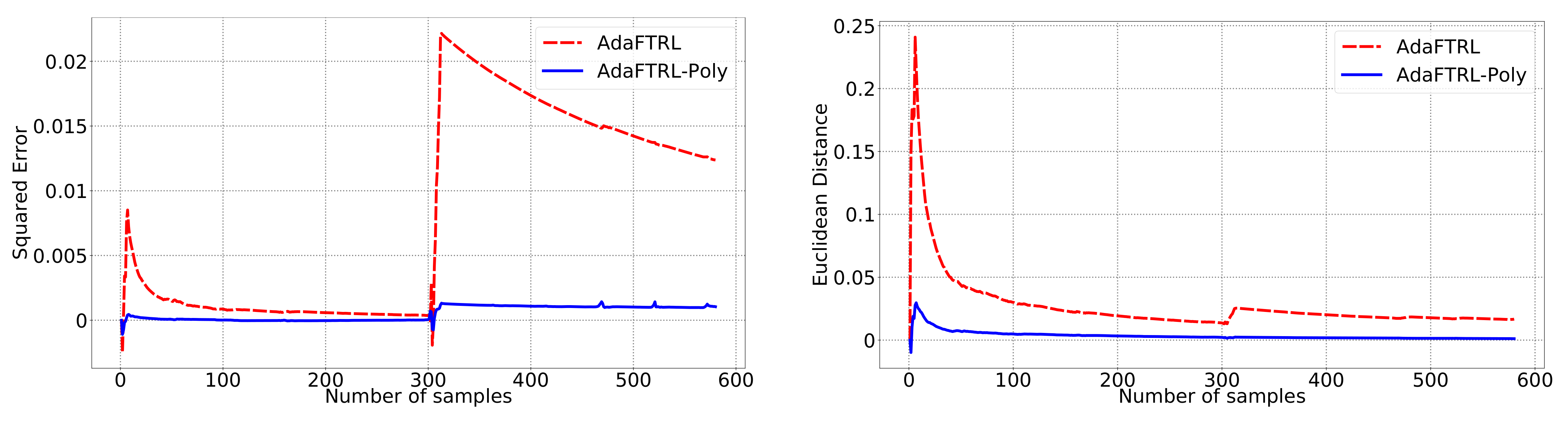
We collect estimates of influenza activity of the northern hemisphere countries, which has an obvious seasonal pattern. In the experiment, we examine the performance of the algorithms for handling regular and predictable changes that occur over a fixed period.

Electricity Demand: Trend and Seasonality

In this setting, we collect monthly load, gross electricity production, net electricity consumption, and gross demand in Turkey from 1976 to 2010. The dataset contains both trend and seasonality.

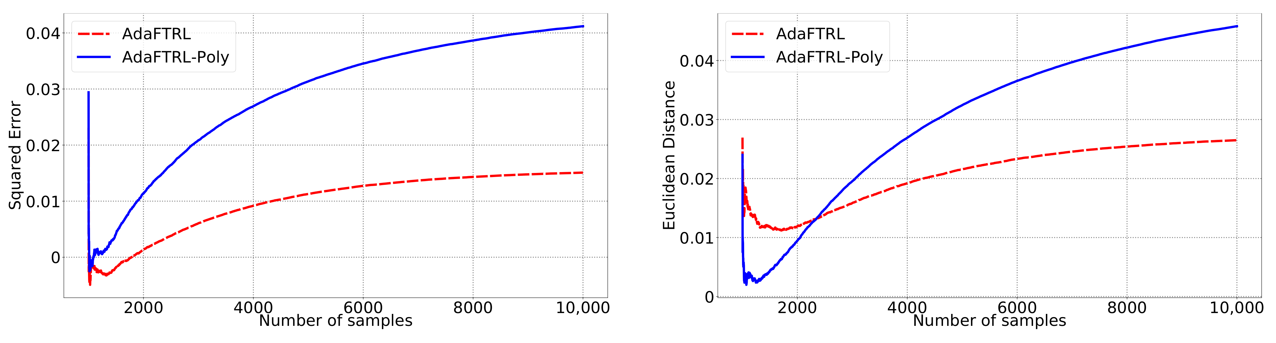
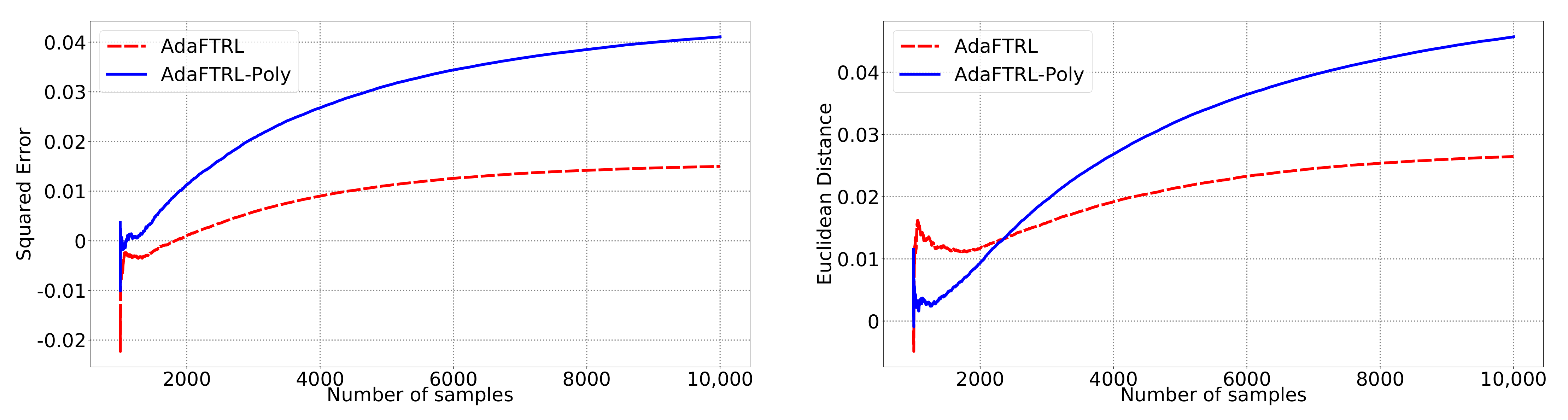
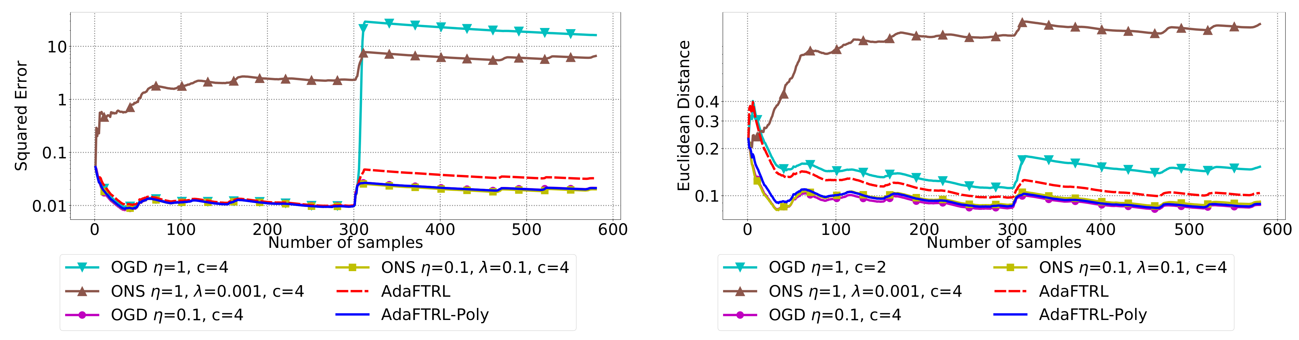
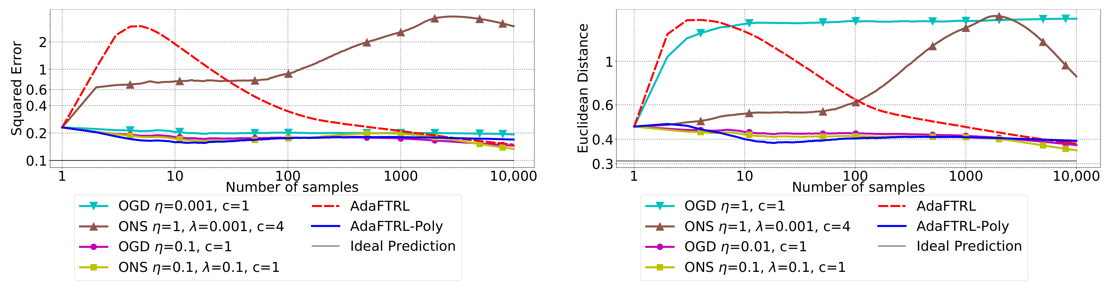
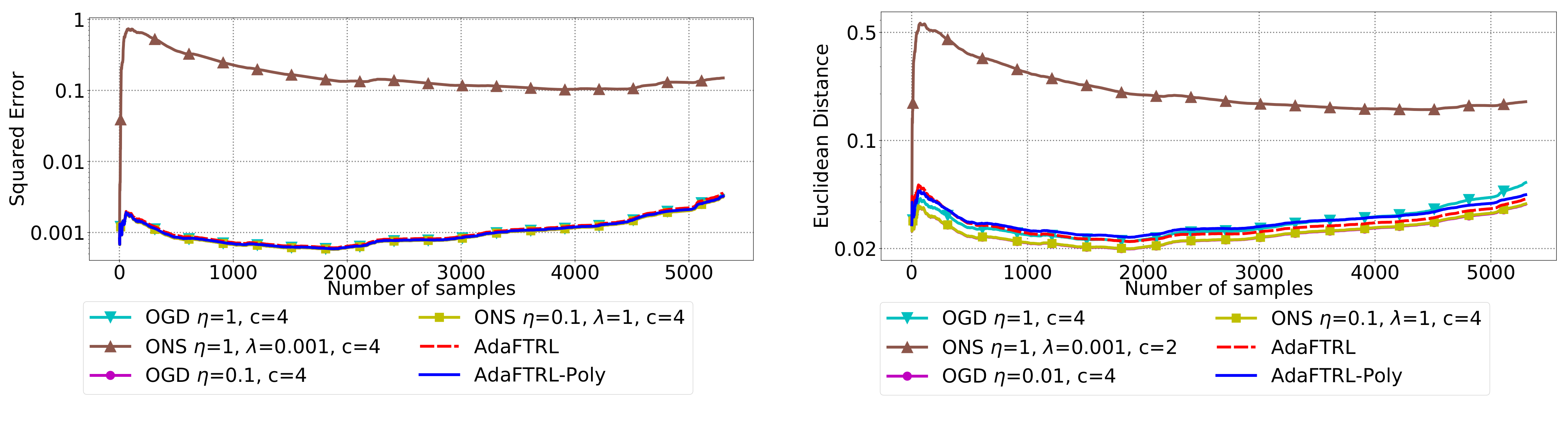
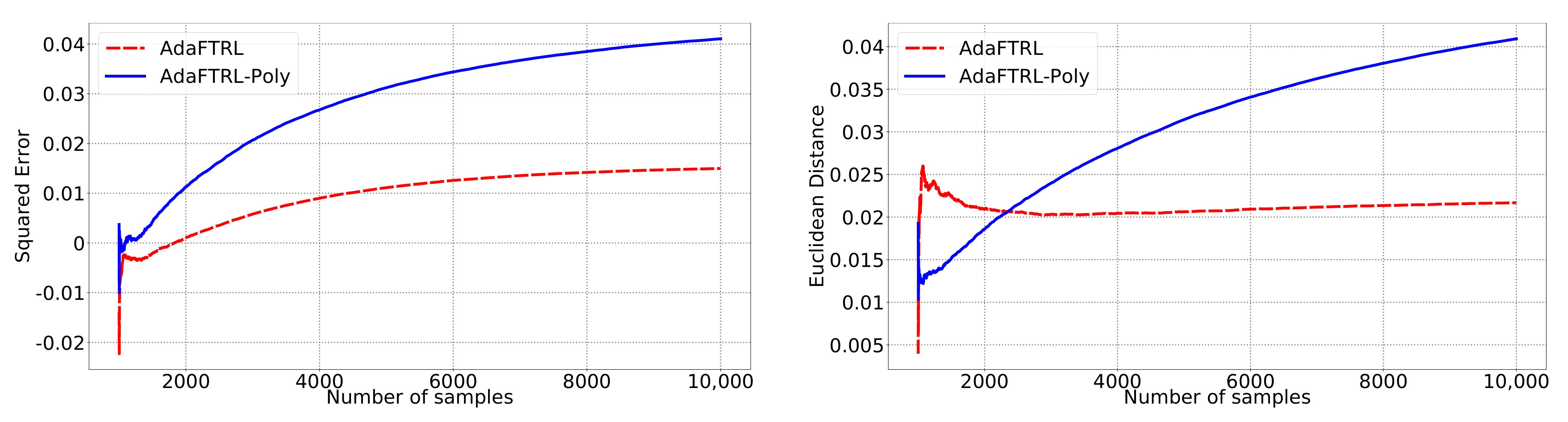
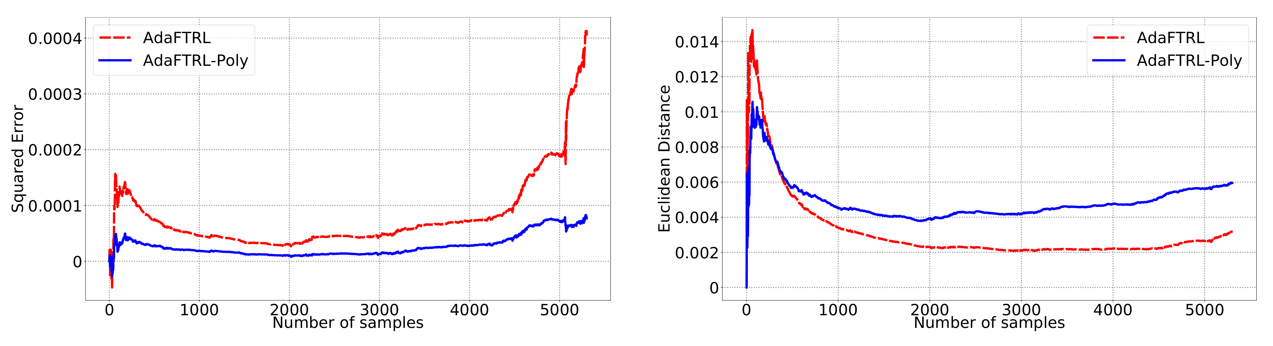
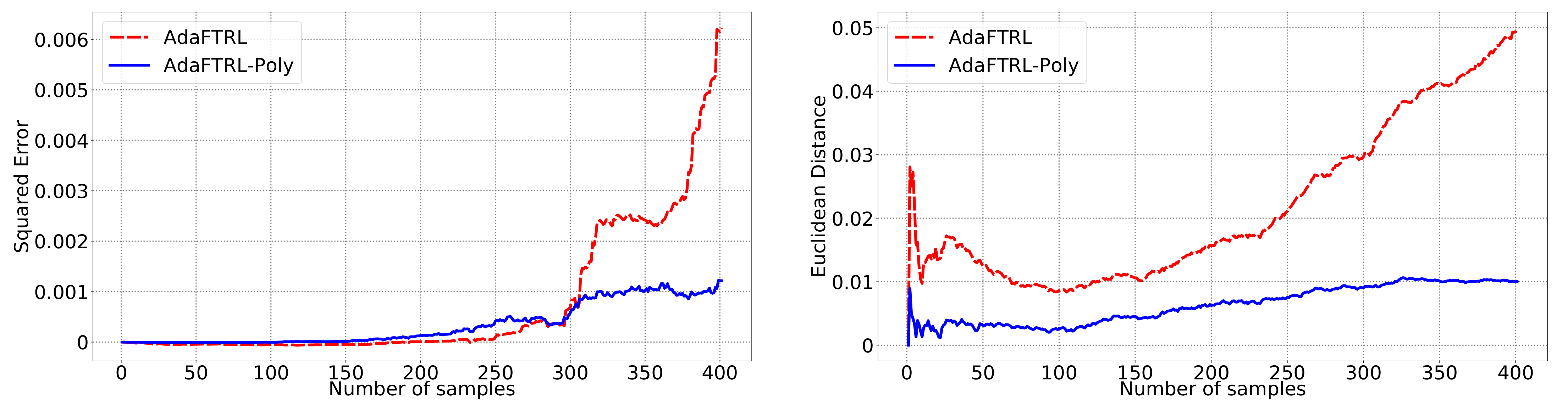
5.2. Experiments for the Slave Algorithms

We first fix $d=1$ and $m=16$ and compare our slave algorithms with ONS and OGD from [9] for squared error $l_t\left({\tilde{X}}_t\right)=\frac{1}{2}{\parallel X_t-{\tilde{X}}_t\parallel }_2^2$ and Euclidean distance $l_t\left({\tilde{X}}_t\right)={\parallel X_t-{\tilde{X}}_t\parallel }_2$. ONS and OGD stack and vectorize the parameter matrices, and incrementally update the vectorized parameter respectively using the following rules

$$w_{t+1}={\Pi }_{\mathcal{W}}(w_t-\eta {(\sum _{s=1}^t{g}_t{g}_t^{\top }+\lambda I)}^{-1}{g}_t)$$

and

$$w_{t+1}={\Pi }_{\mathcal{W}}(w_t-\eta g_t),$$

where $g_t$ is the vectorized gradient at step t, $\mathcal{W}$ is the decision set satisfying ${sup}_{u\in \mathcal{W}}{\parallel u\parallel }_2\le c$, and the operator ${\Pi }_{\mathcal{W}}\left(v\right)$ projects v into $\mathcal{W}$. We select a list of candidate values for each hyperparameter, evaluate their performance on the whole dataset, and select the configuration with the best performance for comparison. Since the synthetic data are generated randomly, we average the results over 20 trials for stability. The corresponding results are shown in Figure 1, Figure 2, Figure 3, Figure 4, Figure 5 and Figure 6 (to amplify the differences of the algorithms, we use $log$ plots for the y-axis for all settings; for the synthetic datasets, we also use $log$ plot for the x-axis, so that the behavior of the algorithms in the first 1000 steps can be better observed). To show the impact of the hyperparameters on the performance of the baseline algorithm, we also plot their performance using sub-optimal configurations. Note that since the error term ${ϵ}_t$ cannot be predicted, an ideal predictor would suffer an average error rate of at least ${\parallel {ϵ}_t\parallel }_2^2$ and ${\parallel {ϵ}_t\parallel }_2$ for the two kinds of loss function. This is known for the synthetic datasets and plotted in the figures.

Figure 1. Results for setting 1 (sanity check), using a stationary ARIMA(5,2,1) model.

Figure 2. Results for setting 2 (time-varying parameters), using a non-stationary ARIMA(5,2,1) model.

Figure 3. Results for setting 3 (time-varying models), using a combination of stationary ARIMA(5,2,1) and ARIMA(5,2,0) models.

Figure 4. Results for stock data.

Figure 5. Results for Google Flu data.

Figure 6. Results for electricity demand data.

In all settings, both AdaFTRL and AdaFTRL-Poly have a performance on par with well-tuned OGD and ONS, which can have extremely bad performance using sub-optimal hyperparameter configurations. In the experiments using synthetic datasets, AdaFTRL suffers large loss at the beginning while generating accurate predictions after 1000 iterations. The relative performances of the proposed algorithms after the first 1000 iterations compared to the best tuned baseline algorithms are plotted in Appendix D. AdaFTRL-Poly has more stable performance compared to AdaFTRL. In the experiment with Google Flu data, all algorithms suffer huge losses around iteration 300 due to an abrupt change in the dataset. OGD and ONS with sub-optimal hyperparameter configurations, despite good performance for the first half of the data, generate very inaccurate predictions after the abrupt change in the dataset. This could lead to a catastrophic failure in practice, when certain patterns do not appear in the dataset collected for hyperparameter tuning. Our algorithms are more robust against this change and perform similarly to OGD and ONS with optimal hyperparameter configurations.

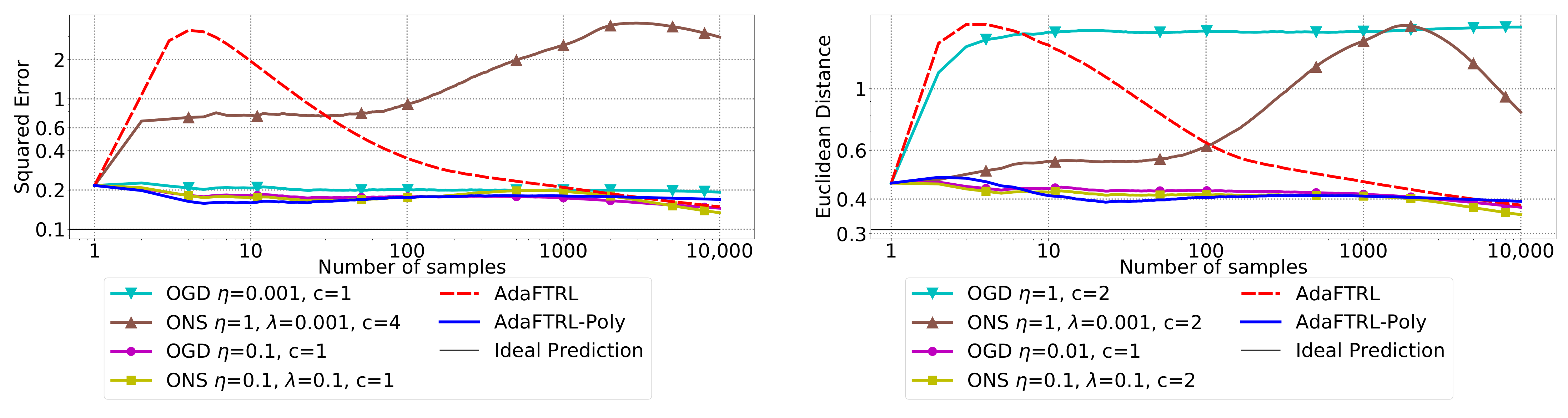
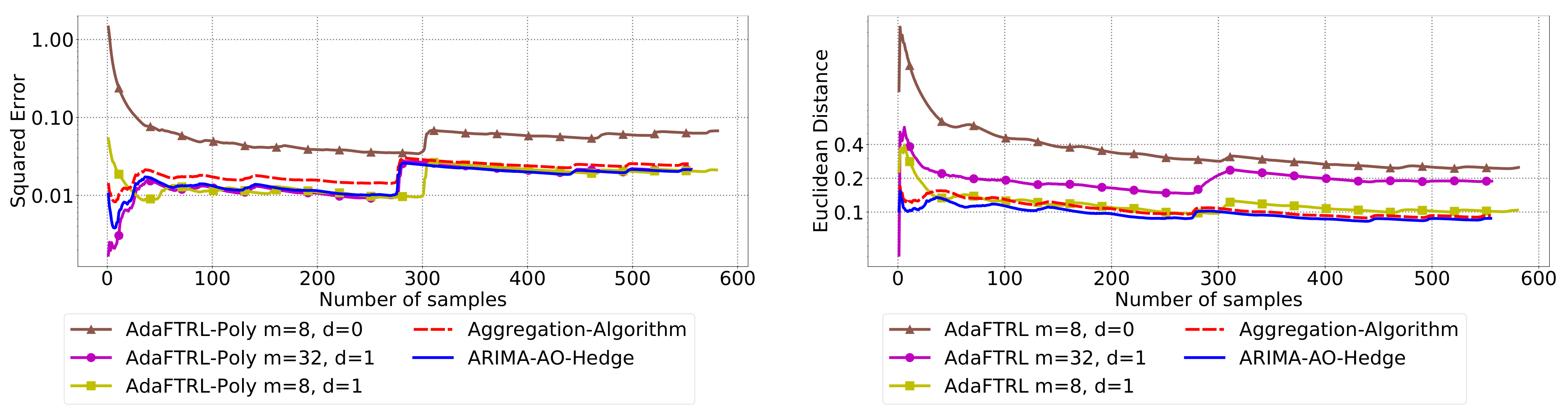
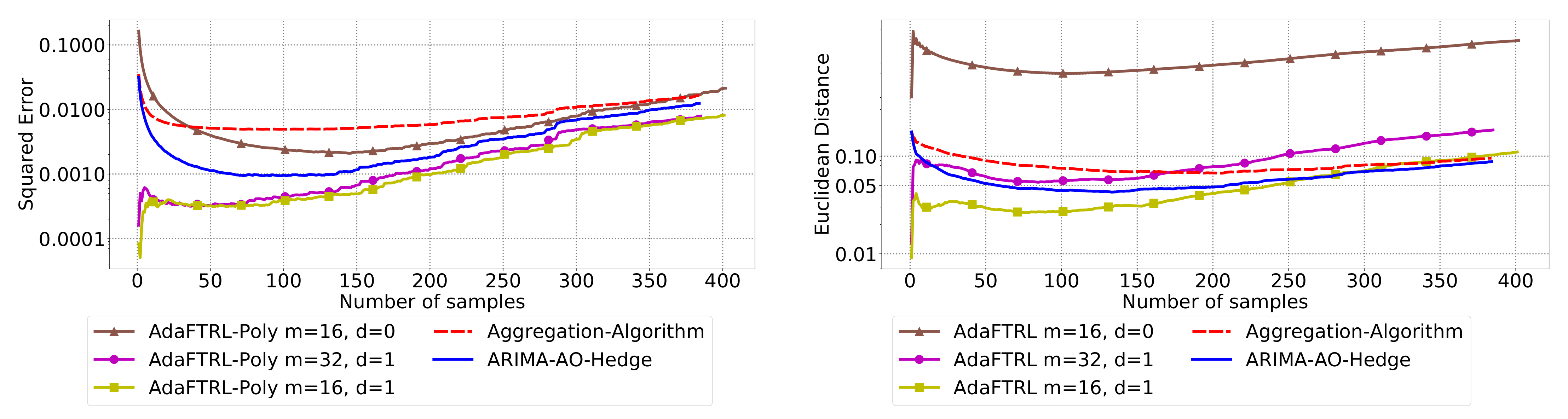
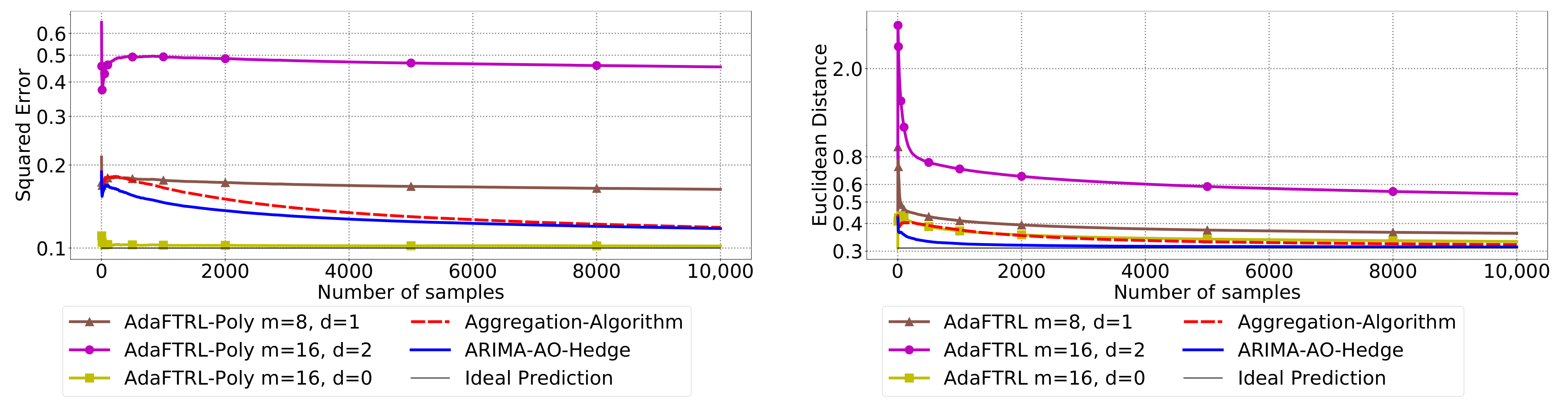
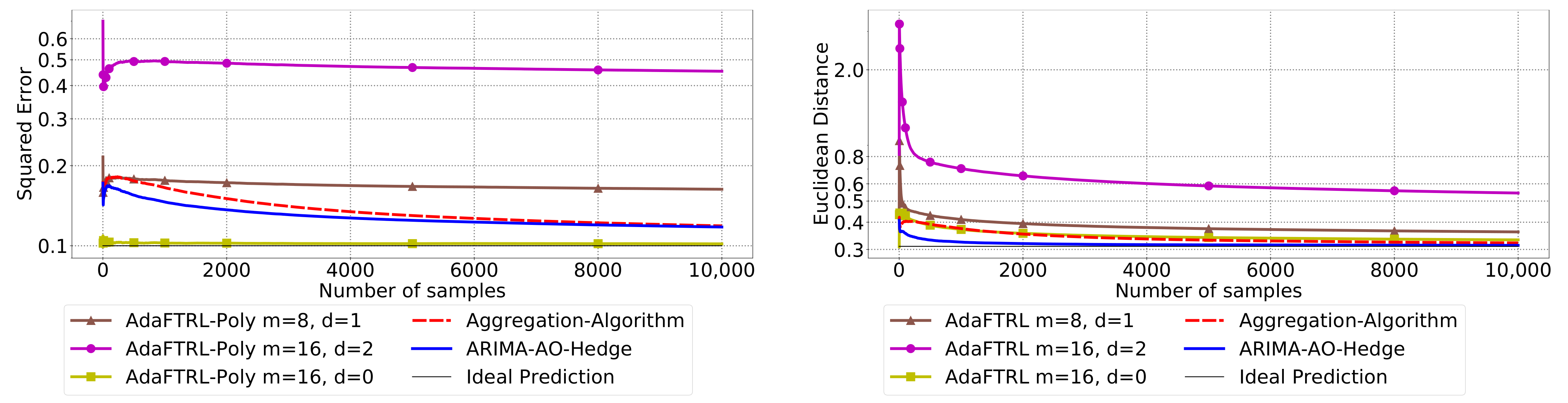
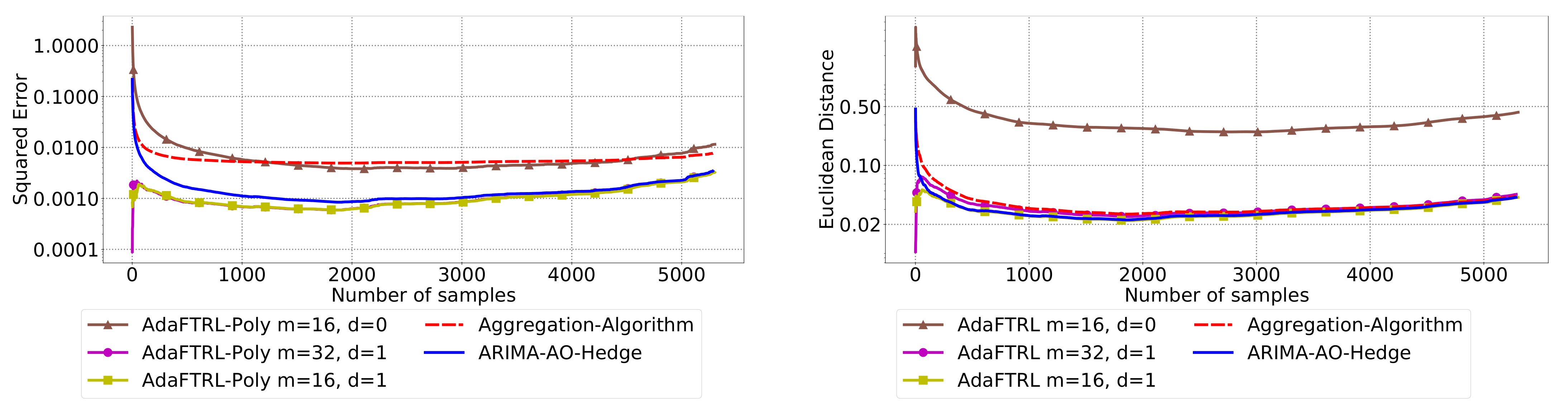
5.3. Experiments for Online Model Selection

The performance of the two-level framework and Algorithm 3 for online model selection is demonstrated in Figure 7, Figure 8, Figure 9, Figure 10, Figure 11 and Figure 12. We simultaneously maintain 96 $AR\left(m\right)$ models of d-th-order differencing for $m=1,\dots 32$ and $d=0,\dots 2$, which are updated by Algorithms 1 and 2 for squared error and Euclidean distance, respectively. The predictions generated by the AR models are aggregated using Algorithm 3 and the aggregation algorithm (AA) introduced in [13] with learning rate set to $\sqrt{T}$. We compare the average losses incurred by the aggregated predictions with those incurred by the best AR model. To show the impact of m and d, we also plot the average loss of some other sub-optimal AR models.

Figure 7. Model selection in setting 1.

Figure 8. Model selection in setting 2.

Figure 9. Model selection in setting 3.

Figure 10. Model selection for stock data.

Figure 11. Model selection for Google Flu.

Figure 12. Model Selection for electricity demand.

In all settings, AO-Hedge outperforms AA, although the differences are very slight in some of the experiments. We would like to stress again that the choice of the hyperparameters has a great impact on the performance of the AR model. In settings 1–3, the AR model with 0-th-order differencing has the best performance, although the data are generated using $d=1$, which suggests that the prior knowledge about the data generation may not be helpful for the model selection in all cases. The experimental results also show that AO-Hedge has a performance similar to the best AR model.

6. Conclusions

We proposed algorithms for fitting ARIMA models in an online manner without requiring prior knowledge or tuning hyperparameters. We showed that the cumulative regret of our method grows sublinearly with the number of iterations and depends on the values of the time series. The comparison study on both synthetic and real-world datasets suggests that the proposed algorithms have a performance on par with the well-tuned state-of-the-art algorithms.

There are still several remaining issues that we want to address in future research. Firstly, it would be interesting to also develop a parameter-free algorithm for the cointegrated vector ARMA model. Secondly, we believe that the strong assumption on the $\beta$ coefficient can be relaxed for multi-dimensional time series by generalizing Lemma 2 in [7]. Furthermore, we are also interested in applying online learning to other time series models such as the (generalized) ARCH model [30]. Finally, the proposed algorithms need to be empirically analyzed using more real-world datasets and loss functions, and compared with more recent predictive models such as recurrent neural networks and the models combining neural networks and ARIMA models [31].