Convergence and Numerical Solution of a Model for Tumor Growth

Abstract

In this paper, we show the application of the meshless numerical method called “Generalized Finite Diference Method” (GFDM) for solving a model for tumor growth with nutrient density, extracellular matrix and matrix degrading enzymes, [recently proposed by Li and Hu]. We derive the discretization of the parabolic–hyperbolic–parabolic–elliptic system by means of the explicit formulae of the GFDM. We provide a theoretical proof of the convergence of the spatial–temporal scheme to the continuous solution and we show several examples over regular and irregular distribution of points. This shows the feasibility of the method for solving this nonlinear model appearing in Biology and Medicine in complicated and realistic domains.

1. Introduction

Cancer includes a large group of diseases that can start in almost any tissue or organ of the body when a cluster of cells starts to grow out of control, going beyond their usual boundaries to invade adjoining areas of the body and spread to other parts of the body. The latter process is known as metastasis and is the main cause of death from cancer. In this process, the ECM (extracellular matrix) composition plays an essential role [1,2]. The ECM is mostly made up of water, fibrous proteins such as collagen, elastin, laminin and proteoglycans. Collagen structure is very important to maintain the ECM function and its degradation by proteases can facilitate the invasion of cancer cells through the basal membrane [3]. Matrix-degrading enzymes (MDE) that break down the ECM can lead to invasion, where either individual or collections of cancerous cells can escape or separate from the tumor and migrate through the surrounding tissue. Thus these cells can also enter through the blood or lymphatic vessels and travel to distant locations which can develop into metastasis. Tumor cells also modify the behavior of the neighboring cells, so that they can serve as nutrient donors for cancer cell proliferation and spreading. Hence, an alteration in the nutrient density within the tumor microenvironment has been associated with malignancy progression and death [4].

Understanding how the mechanical microenvironment regulates cancer cell development that ends in metastasis represents a newly developing study model. The research related to this new model could lead to discovering better anti-metastasis therapeutics.

Over the last few years, mathematical modeling has played an essential role in Cancer research. Particularly, an increasing number of mathematical models describing tumour growth have been developed.

To describe the process and the related mechanism, we study a mathematical model for the influence of the extracellular matrix (ECM) on tumour evolution in terms of a system of partial differential equations, i.e., parabolic equations and a hyperbolic equation for nutrient density, MDE and ECM concentration. Moreover, it contains a non-constant coefficient $\mu \left(E\right)$ and allows for the movement of ECM fibres. The model is more reasonable and presents a realistic scenario, nonetheless it leads to a more difficult problem to analyse.

In this paper, we propose a model that describes the evolution with tumor microenvironment involving nutrient density, extracellular matrix and matrix degrading enzymes, which satisfy a coupled system of PDEs as follows:

$$\left\{\begin{array}{cc}c{\displaystyle \frac{\partial \sigma }{\partial t}}=\mathsf{\Delta }\sigma -\nu \sigma ,\hfill & \overrightarrow{x}\in \Omega ,t>0,\hfill \\ {\displaystyle \frac{\partial E}{\partial t}}+div(E·\overrightarrow{V})=-\gamma mE+\varphi \left(E\right),\hfill & \overrightarrow{x}\in \Omega ,t>0,\hfill \\ {\displaystyle \frac{\partial m}{\partial t}}=D\mathsf{\Delta }m+\alpha -\beta m,\hfill & \overrightarrow{x}\in \Omega ,t>0,\hfill \\ \overrightarrow{V}=-f\left(E\right)\nabla p,\hfill & \overrightarrow{x}\in \Omega ,\hfill \\ div\overrightarrow{V}=g\left(E\right)(\sigma -\overline{\sigma }),\hfill & \overrightarrow{x}\in \Omega ,\hfill \end{array}\right.$$

(1)

with boundary conditions

$$\left\{\begin{array}{cc}\sigma =const.,\hfill & \overrightarrow{x}\in \partial \Omega ,\hfill \\ {\displaystyle \frac{\partial E}{\partial \overrightarrow{n}}}=0,\hfill & \overrightarrow{x}\in \partial \Omega ,\hfill \\ {\displaystyle \frac{\partial m}{\partial \overrightarrow{n}}}=0,\hfill & \overrightarrow{x}\in \partial \Omega ,\hfill \\ p=const.,\hfill & \overrightarrow{x}\in \partial \Omega \hfill \end{array}\right.$$

(2)

and initial conditions: ${\sigma }_0\left(\overrightarrow{x}\right)$, $E_0\left(\overrightarrow{x}\right)$, $m_0\left(\overrightarrow{x}\right)$, $p_0\left(\overrightarrow{x}\right)$. A range of values for the parameters of the problem can be found in [5,6] as well as in [1].

The first diffusion equation in (1) describes the evolution of the nutrient $\sigma$ within the tumor, c is the ratio of the nutrient diffusion time scale to the tumor growth (e.g., tumor doubling) time scale and $\nu \sigma$ describes the rate of consumption by the tumor. For the obtaining of the second equation in (1), it is taken into account that the concentration of the ECM in the system is governed by contributions from three factors: haptotaxis, degrading and production.

E is the extracellular matrix, $\overrightarrow{V}$ represents the velocity of proliferating cells, the term $div(E·\overrightarrow{V})$ is the movement of ECM owing to the cell proliferation $\overrightarrow{V}$, $-\gamma mE$ represents the degrading of ECM by MDE, where m is the concentration of MDE and $\varphi \left(E\right)$ is a positive term representing reorganization of ECM. Since the growth rate of ECM is smaller when the ECM is denser, $\varphi \left(E\right)$ is a positive monotone decreasing function of E.

It is well-known that the matrix degrading enzymes (MDE) is produced by the tumor to degrade ECM so that the cells can escape. In the MDE’s equation in (1) $\mathsf{\Delta }m$ represents diffusion, D is the constant diffusion coefficient, $\alpha$ is a constant production rate by the tumor and $-\beta m$ represents natural decay. The fourth and fifth equations in (1) are deduced by employing the Darcy’s law and the conservation of mass: p the pressure within the tumor resulting from this proliferation, the coefficient $f\left(E\right)$ depends on the density of the porous medium, representing a mobility that reflects the combined effects of cell-cell and cell-matrix adhesion, i.e., $f\left(E\right)$ depends on the amount of ECM present in the tumor. In the last equation $S=g\left(E\right)(\sigma -\overline{\sigma })$ is a linear approximation for the proliferation S, where $g\left(E\right)\sigma$ represents the growth rate and $g\left(E\right)\overline{\sigma }$ is the death rate from apoptosis, $g\left(E\right)$ is a function of the ECM concentration. Hence, it yields $div\overrightarrow{V}=S$.

Operating with the fourth and fifth equations of (1), the system can be rewritten:

$$\left\{\begin{array}{cc}c{\displaystyle \frac{\partial \sigma }{\partial t}}=\mathsf{\Delta }\sigma -\nu \sigma ,\hfill & \overrightarrow{x}\in \Omega ,t>0,\hfill \\ {\displaystyle \frac{\partial E}{\partial t}}-f\left(E\right)\nabla E·\nabla p+Eg\left(E\right)(\sigma -\overline{\sigma })=-\gamma mE+\varphi \left(E\right),\hfill & \overrightarrow{x}\in \Omega ,t>0,\hfill \\ {\displaystyle \frac{\partial m}{\partial t}}=D\mathsf{\Delta }m+\alpha -\beta m,\hfill & \overrightarrow{x}\in \Omega ,t>0,\hfill \\ 0=\mathsf{\Delta }p+{\displaystyle \frac{g\left(E\right)}{f\left(E\right)}}(\sigma -\overline{\sigma })-{\displaystyle \frac{f^{\prime }\left(E\right)}{f\left(E\right)}}\nabla E·\nabla p,\hfill & \overrightarrow{x}\in \Omega .\hfill \end{array}\right.$$

(3)

In the system under consideration, c, $\mu$, $\gamma$, D $\alpha$, $\beta$, $\overline{\sigma }$ are constants, as we have previously detailed. The functions f and g are decreasing, strictly positive and bounded. The function $\varphi$ is positive and decreasing.

The importance of models such as the above, which present a high degree of plausability, lies in their application in sciences such as biology and medicine. Their high nonlinearity, as well as the use of complicated and non-uniform domains, makes necessary the implementation of meshless methods. The Generalized Finite Difference Method (GFDM) is a meshless numerical method based on the Taylor expansion and moving least squares. This method allows us to find the discrete solution of the above system over non-uniform grids. The GFDM provides a simple discretization of the spatial derivatives at some point in terms of the values of the solution at the surrounding ones. These aspects (as well as the small number of points per star) have meant that the method has recently been used widely in [7,8] and is currently expanding [9].

The paper has the following structure: we show the fundamentals of the GFDM for completeness in Section 2. Section 3 is devoted to the proof of the convergence of the discrete solution to the continuous one of the system. We perform in the fourth section three examples with different geometries. We present in the last section some conclusions.

2. Fundamentals of the GFDM

Let $\Omega \subset {\mathbb{R}}^2$ be a bounded domain and

$$M=\{{\mathbf{x}}_1,\dots ,{\mathbf{x}}_N\}\subset \Omega$$

a discretization of the domain $\Omega$ with N points. Each point of the discretization M is denoted as a node.

For each one of the nodes of the domain $\Omega$, $E_s$-star is defined as a set of selected points $E_s=\{{\mathbf{x}}_0;{\mathbf{x}}_1,\dots ,{\mathbf{x}}_s\}\subset M$ with the central node ${\mathbf{x}}_0\in M$ and ${\mathbf{x}}_i(i=1,\dots ,s)\in M$ is a set of points located in the neighbourhood of ${\mathit{x}}_{\mathbf{0}}$. In order to select the points, different criteria as four quadrants or distance [10], can be used.

Consider an $E_s$-star with the central node ${\mathbf{x}}_0$, where $(x_0,y_0)$ are the coordinates of the central node, $(x_i,y_i)$ are the coordinates of the $i^{th}$ node in the $E_s$-star, and $h_i=x_i-x_0$ and $k_i=y_i-y_0$.

If $U_0=U\left({\mathbf{x}}_0\right)$ is the value of the function at the central node of the star and $U_i=U\left({\mathbf{x}}_i\right)$ are the function values at the rest of the nodes, with $i=1,\dots ,s$, then, according to the Taylor series expansion:

$$U_i=U_0+h_i{\displaystyle \frac{\partial U_0}{\partial x}}+k_i{\displaystyle \frac{\partial U_0}{\partial y}}+{\displaystyle \frac{1}{2}}\left(h_i^2{\displaystyle \frac{{\partial }^2{U}_0}{\partial x^2}}+k_i^2{\displaystyle \frac{{\partial }^2{U}_0}{\partial y^2}}+2h_i{k}_i{\displaystyle \frac{{\partial }^2{U}_0}{\partial x\partial y}}\right)+\dots ,.$$

(4)

with $i=1,\dots ,s$. We define:

$${{\mathbf{c}}_{\mathbf{i}}}^T=\left\{h_i,k_i,\frac{h_i^2}{2},\frac{k_i^2}{2},h_i{k}_i\right\},$$

(5)

$${\mathit{D}}^T=\left\{\frac{\partial u_0}{\partial x},\frac{\partial u_0}{\partial y},\frac{{\partial }^2{u}_0}{\partial x^2},\frac{{\partial }^2{u}_0}{\partial y^2},\frac{{\partial }^2{u}_0}{\partial x\partial y}\right\}.$$

(6)

If in (4) the higher than second order terms are ignored, a second order approximation for the function $U_i$ is obtained. We denote it by $u_i$. It is then possible to define the function $B\left(u\right)$ as

$${\displaystyle B\left(u\right)=\sum _{i=1}^s{\left[(u_0-u_i)+h_i\frac{\partial u_0}{\partial x}+k_i\frac{\partial u_0}{\partial y}+\frac{1}{2}(h_i^2\frac{{\partial }^2{u}_0}{\partial x^2}+k_i^2\frac{{\partial }^2{u}_0}{\partial y^2}+2h_i{k}_i\frac{{\partial }^2{u}_0}{\partial x\partial y})\right]}^2{w}_i^2,}$$

(7)

where $w_i=w(h_i,k_i)$ are positive symmetrical weighting functions decreasing in magnitude as the distance to the center increases [10], of decreasing monotonically in magnitude as the distance to the center of the weighting function increases (see also Levin [11] for more details of this election).

Some weighting functions as potential ${\displaystyle \frac{1}{dis{t}^n}}$ or exponential $exp(-n\left(dis{t}^2\right))$ can be used [12], where $n\in \mathbb{N}$. We minimize the norm given by (7) with respect to the partial derivatives by considering the following linear system

$$\mathit{A}(h_i,k_i,w_i)\mathit{D}=\mathit{b}(h_i,k_i,w_i,u_0,u_i),$$

(8)

where

$$\mathit{A}=\left(\begin{array}{cccc}{h}_1& h_2& \dots & h_s\\ k_1& k_2& \dots & k_s\\ ⋮& ⋮& ⋮& ⋮\\ h_1{k}_1& h_2{k}_2& \dots & h_s{k}_s\end{array}\right)\left(\begin{array}{cccc}{\omega }_1^2& & & \\ & {\omega }_2^2& & \\ & & \dots & \\ & & & {\omega }_s^2\end{array}\right)\left(\begin{array}{cccc}{h}_1& k_1& \dots & h_1{k}_1\\ h_2& k_2& \dots & h_2{k}_2\\ ⋮& ⋮& ⋮& ⋮\\ h_s& k_s& \dots & h_s{k}_s\end{array}\right)$$

(9)

and

$$\begin{array}{cc}\hfill {\mathit{b}}^T=& {\displaystyle \{\sum _{i=1}^s(-u_0+u_i)h_i{w}_i^2,\sum _{i=1}^s(-u_0+u_i)k_i{w}_i^2,\sum _{i=1}^s(-u_0+u_i)\frac{h_i^2}{2}{w}_i^2,}\hfill \\ & {\displaystyle \sum _{i=1}^s(-u_0+u_i)\frac{k_i^2}{2}{w}_i^2,\sum _{i=1}^s(-u_0+u_i)h_i{k}_i{w}_i^2\}.}\hfill \end{array}$$

Positive definiteness of $\mathit{A}$ and the consistency of the approximation is proved in [13]. Thus, spatial derivatives using GFD [12,13] are denoted by

$$\left\{\begin{array}{c}{\displaystyle {\displaystyle \frac{\partial u(x_0,y_0,n\mathsf{\Delta }t)}{\partial x}}=-{\lambda }_{10}{u}_0^n+\sum _{i=1}^s{\lambda }_{1i}{u}_i^n+\mathcal{O}(h_i^2,k_i^2),}\hfill \\ {\displaystyle {\displaystyle \frac{\partial u(x_0,y_0,n\mathsf{\Delta }t)}{\partial y}}=-{\lambda }_{20}{u}_0^n+\sum _{i=1}^s{\lambda }_{2i}{u}_i^n+\mathcal{O}(h_i^2,k_i^2),}\hfill \\ {\displaystyle {\displaystyle \frac{{\partial }^{2}u(x_0,y_0,n\mathsf{\Delta }t)}{\partial x^2}}+{\displaystyle \frac{{\partial }^{2}u(x_0,y_0,n\mathsf{\Delta }t)}{\partial y^2}}=-{\lambda }_0{u}_0^n+\sum _{i=1}^s{\lambda }_i{u}_i^n+\mathcal{O}(h_i^2,k_i^2),}\hfill \end{array}\right.$$

(10)

with

$${\displaystyle {\lambda }_{10}=\sum _{i=1}^s{\lambda }_{1i},{\lambda }_{20}=\sum _{i=1}^s{\lambda }_{2i},{\lambda }_0=\sum _{i=1}^s{\lambda }_i.}$$

Finally, the time derivative is approximated as follows

$$\frac{\partial u}{\partial t}({\mathbf{x}}_0,n\mathsf{\Delta }t)=\frac{u({\mathbf{x}}_0,(n+1)\mathsf{\Delta }t)-u({\mathbf{x}}_0,n\mathsf{\Delta }t)}{\mathsf{\Delta }t}+\mathcal{O}\left(\mathsf{\Delta }t\right).$$

(11)

GFD Scheme for System (3)

Let $\widehat{\sigma }$, $\widehat{m}$, $\widehat{E}$ be aproximated solution of the system (3), that can be discretized as:

$$\left\{\begin{array}{c}{\displaystyle \frac{{\widehat{\sigma }}_0^{n+1}-{\widehat{\sigma }}_0^n}{\mathsf{\Delta }t}}={\displaystyle \frac{1}{c}}\left({\displaystyle -{\lambda }_0{\widehat{\sigma }}_0^n+\sum _{i=1}^s{\lambda }_i{\widehat{\sigma }}_i^n}\right)-\nu {\widehat{\sigma }}_0^n,\hfill \\ \overrightarrow{V}=-\overline{\mu }\left({\widehat{E}}_0^n\right)\left({\displaystyle \frac{\partial p}{\partial x}}{|}_0^n,{\displaystyle \frac{\partial p}{\partial y}}{|}_0^n\right),\hfill \\ div\overrightarrow{V}=\mu \left({\widehat{E}}_0^n\right)({\widehat{\sigma }}_0^n-\overline{\sigma }),\hfill \\ {\displaystyle \frac{{\widehat{E}}_0^{n+1}-{\widehat{E}}_0^n}{\mathsf{\Delta }t}}+div(\widehat{E}·\overrightarrow{V})=-\gamma \widehat{m}\widehat{E}+\varphi \left(\widehat{E}\right),\hfill \\ {\displaystyle \frac{{\widehat{m}}_0^{n+1}-{\widehat{m}}_0^n}{\mathsf{\Delta }t}}=D\left({\displaystyle -{\lambda }_0{\widehat{m}}_0^n+\sum _{i=1}^s{\lambda }_i{\widehat{m}}_i^n}\right)+\alpha -\beta {\widehat{m}}_0^n.\hfill \end{array}\right.$$

(12)

Using the relation

$$div\left(E·\overrightarrow{V}\right)=\nabla E·\overrightarrow{V}+Ediv\left(\overrightarrow{V}\right)=\nabla E·\overrightarrow{V}+E\mu \left(E\right)(\sigma -\overline{\sigma }),$$

(13)

we get

$$\begin{array}{cc}\hfill {\displaystyle \frac{{\widehat{E}}_0^{n+1}-{\widehat{E}}_0^n}{\mathsf{\Delta }t}}& {\displaystyle -\mu \left({\widehat{E}}_0^n\right)\left(-{\lambda }_{10}{\widehat{E}}_0^n+\sum _{i=1}^s{\lambda }_{1i}{\widehat{E}}_i^n\right){\displaystyle \frac{\partial p}{\partial x}}{|}_0^n}\hfill \\ & {\displaystyle -\mu \left({\widehat{E}}_0^n\right)\left(-{\lambda }_{20}{\widehat{E}}_0^n+\sum _{i=1}^s{\lambda }_{2i}{\widehat{E}}_i^n\right){\displaystyle \frac{\partial p}{\partial y}}{|}_0^n+{\widehat{E}}_0^n\mu \left({\widehat{E}}_0^n\right)({\widehat{\sigma }}_0^n-\overline{\sigma })}\hfill \\ & =-\gamma {\widehat{m}}_0^n{\widehat{E}}_0^n+\varphi \left({\widehat{E}}_0^n\right),\hfill \end{array}$$

(14)

$$\begin{array}{c}\hfill \left\{\begin{array}{c}{\displaystyle {\widehat{\sigma }}_0^{n+1}={\widehat{\sigma }}_0^n\left[1-{\displaystyle \frac{\mathsf{\Delta }t}{c}}\left({\lambda }_0+\nu \right)\right]+{\displaystyle \frac{\mathsf{\Delta }t}{c}}\sum _{i=1}^s{\lambda }_i{\widehat{\sigma }}_i^n,}\hfill \\ {\displaystyle {\widehat{m}}_0^{n+1}={\widehat{m}}_0^n\left[1-\mathsf{\Delta }t\left(D{\lambda }_0+\beta \right)\right]+D\mathsf{\Delta }t\sum _{i=1}^s{\lambda }_i{\widehat{m}}_i^n+\alpha \mathsf{\Delta }t,}\hfill \\ \overrightarrow{V}=-\overline{\mu }\left(\widehat{E_0^n}\right)\left({\displaystyle \frac{\partial p}{\partial x}}{|}_0^n{\displaystyle \frac{\partial p}{\partial y}}{|}_0^n\right),\hfill \\ {\widehat{E}}_0^{n+1}={\widehat{E}}_0^n\left[1-\mathsf{\Delta }t\left(\mu \left({\widehat{E}}_0^n\right)({\widehat{\sigma }}_0^n-\overline{\sigma })+\gamma {\widehat{m}}_0^n\right)\right]+\mathsf{\Delta }t(\mu \left({\widehat{E}}_0^n\right)\left({\displaystyle -{\lambda }_{10}{\widehat{E}}_0^n+\sum _{i=1}^s{\lambda }_{1i}{\widehat{E}}_i^n}\right){\displaystyle \frac{\partial p}{\partial x}}{|}_0^n\hfill \\ +\mathsf{\Delta }t\mu \left({\widehat{E}}_0^n\right)\left({\displaystyle -{\lambda }_{20}{\widehat{E}}_0^n+\sum _{i=1}^s{\lambda }_{2i}{\widehat{E}}_i^n}\right){\displaystyle \frac{\partial p}{\partial y}}{|}_0^n+\mathsf{\Delta }t\varphi \left({\widehat{E}}_0^n\right).\hfill \end{array}\right.\end{array}$$

(15)

3. Convergence

Some basic and previous results are needed in order to obtain the proof of the conditional convergence of the methods. For completeness, we reproduce them:

Lemma 1

([14]). Let be a matrix $\mathcal{N}\in {\mathfrak{M}}_{n\times n}\left(\mathbb{R}\right)$. If there exists some matrix norm verifying $\parallel \mathcal{N}\parallel <1,$ then

$$\underset{k\to \infty }{lim}{\mathcal{N}}^k=\mathbf{0}.$$

Lemma 2

([14]). Assume $\mathcal{N}\in {\mathfrak{M}}_{n\times n}\left(\mathbb{R}\right)$, then the following issues are equivalent:

(i) 

${\displaystyle \underset{k\to \infty }{lim}{\mathcal{N}}^k=\mathbf{0},}$

(ii) 

$\rho \left(\mathcal{N}\right)<1$,

where $\rho (·)$ stands for the spectral radius.

Our numerical convergence result is the following.

Theorem 1.

Let σ, m, E be the exact solution of (3), and μ and p are differentiable functions. If

$$\begin{array}{cc}& {\displaystyle •\sum _{i=1}^s\left|{\lambda }_i\right|-{\lambda }_0-\nu <0,}\hfill \\ & {\displaystyle •D(\sum _{i=1}^s|{\lambda }_i|-{\lambda }_0)-\beta <0}\hfill \\ & •|B_2|+F_1+F_2-B_1<0,\hfill \end{array}$$

then the GFD explicit scheme (15) is convergent if

$$\mathsf{\Delta }t\le 2min\left\{{\displaystyle \frac{c}{{\displaystyle \sum _{i=1}^s\left|{\lambda }_i\right|+{\lambda }_0+\nu }}},{\displaystyle \frac{1}{B_1+\left|B_2\right|+F_1+F_3}},{\displaystyle \frac{1}{{\displaystyle {\lambda }_0+\sum _{i=1}^s{\lambda }_i}}}\right\},$$

where

$$\begin{array}{cc}\hfill B_1:=& [\left({\displaystyle {\lambda }_{10}\mu +{\lambda }_{10}\widehat{E_0^n}{\mu }^{\prime }+{\mu }^{\prime }\sum _{i=1}^s{\lambda }_{1i}{E}_i^n}\right){\displaystyle \frac{\partial p}{\partial x}}{|}_0^n+\left({\displaystyle -{\lambda }_{20}\mu +{\lambda }_{20}\widehat{E_0^n}{\mu }^{\prime }+{\mu }^{\prime }\sum _{i=1}^s{\lambda }_{2i}{E}_i^n}\right){\displaystyle \frac{\partial p}{\partial y}}{|}_0^n\hfill \\ \hfill & +\mu {\sigma }_0^n+{\mu }^{\prime }{\widehat{E}}_0^n{\widehat{\sigma }}_0^n+\mu \overline{\sigma }+{\mu }^{\prime }{\widehat{E}}_0^n+\gamma {\widehat{m}}_0^n],\hfill \\ \hfill B_2:& =({\displaystyle \frac{\partial p}{\partial x}}{|}_0^n{\displaystyle \sum _{i=1}^s{\lambda }_{1i}{\xi }_i^n}+{\displaystyle \frac{\partial p}{\partial y}}{|}_0^n\left.{\displaystyle \sum _{i=1}^s{\lambda }_{2i}{\xi }_i^n}\right),\hfill \\ \hfill F_1:& =\left|\mu {\widehat{E}}_0^n\right|\mathsf{\Delta }t,\hfill \\ \hfill F_2:& =\left|\gamma E_0^n\right|\mathsf{\Delta }t.\hfill \end{array}$$

(16)

Proof. 

We call ${\rho }_j^n={\widehat{\sigma }}_j^n-{\sigma }_j^n$, ${\eta }_j^n={\widehat{m}}_j^n-m_j^n$, ${\xi }_j^n={\widehat{E}}_j^n-E_j^n$. Let us take the difference between the expressions of the numerical solution given by the GFD scheme (15) and the expression for the exact solution of (3). Since the function $\mu \left(E\right)$ is differentiable, we apply the Mean Value Theorem and by operating, we obtain the following:

$$\begin{array}{cc}\hfill {\rho }_0^{n+1}& {\displaystyle ={\rho }_0^n\left[1-\frac{\mathsf{\Delta }t}{c}\left({\lambda }_0+\nu \right)\right]+\frac{\mathsf{\Delta }t}{c}\sum _{i=1}^s{\lambda }_i{\rho }_i^n}\hfill \\ \hfill {\eta }_0^{n+1}& {\displaystyle ={\eta }_0^n\left[1-\mathsf{\Delta }t\left(D{\lambda }_0+\beta \right)\right]+D\mathsf{\Delta }t\sum _{i=1}^s{\lambda }_i{\eta }_i^n}\hfill \\ \hfill {\xi }_0^{n+1}& {\displaystyle ={\xi }_0^n\{1-\mathsf{\Delta }t[{\displaystyle \frac{\partial p}{\partial x}}{|}_0^n\left(\mu {\lambda }_{10}+{\mu }^{\prime }{\lambda }_{10}{\widehat{E}}_0^n+{\mu }^{\prime }\sum _{i=1}^s{\lambda }_{1i}{E}_i^n\right)}\hfill \\ \hfill & {\displaystyle +{\displaystyle \frac{\partial p}{\partial y}}{|}_0^n\left.\left(\mu {\lambda }_{20}+{\mu }^{\prime }{\lambda }_{20}{\widehat{E}}_0^n+{\mu }^{\prime }\sum _{i=1}^s{\lambda }_{2i}{E}_i^n\right)+\mu {\sigma }_0^n+{\mu }^{\prime }{\widehat{E}}_0^n{\widehat{\sigma }}_0^n+\mu \overline{\sigma }+\gamma {\widehat{m}}_0^n\right]\}}\hfill \\ \hfill & {\displaystyle +\mathsf{\Delta }t{\displaystyle \frac{\partial p}{\partial x}}{|}_0^n\sum _{i=1}^s{\lambda }_{1i}{\xi }_i^n+\mathsf{\Delta }t{\displaystyle \frac{\partial p}{\partial y}}{|}_0^n\sum _{i=1}^s{\lambda }_{2i}{\xi }_i^n-\mathsf{\Delta }t\mu {\widehat{E}}_0^n{\rho }_0^n-\mathsf{\Delta }t\gamma {\widehat{E}}_0^n{\eta }_0^n.}\hfill \end{array}$$

(17)

We now take bounds and call ${\displaystyle {\tilde{\rho }}^n=\underset{i=0,\dots ,s}{max}\left\{\right|{\tilde{\rho }}_i^n\left|\right\}}$ (the same applies for ${\tilde{\xi }}^n$ and ${\tilde{\eta }}^n$). Then, we have

$$\begin{array}{cc}\hfill {\tilde{\rho }}^{n+1}& {\displaystyle \le {\tilde{\rho }}^n\left[\left|1-\frac{\mathsf{\Delta }t}{c}\left({\lambda }_0+\nu \right)\right|+\frac{\mathsf{\Delta }t}{c}\sum _{i=1}^s\left|{\lambda }_i\right|\right]=A_1{\tilde{\rho }}^n}\hfill \\ \hfill .{\tilde{\eta }}^{n+1}& {\displaystyle \le {\tilde{\eta }}^n\left[\left|1-\mathsf{\Delta }t\left(D{\lambda }_0+\beta \right)\right|+D\mathsf{\Delta }t\sum _{i=1}^s\left|{\lambda }_i\right|\right]=C_1{\tilde{\eta }}^n}\hfill \\ \hfill .{\tilde{\xi }}^{n+1}& \le {\tilde{\xi }}^n\left[\left|1-\mathsf{\Delta }t{B}_1\right|+\mathsf{\Delta }t\left|B_2\right|\right]+{\tilde{\rho }}_0^n\mathsf{\Delta }t\left|\mu {\widehat{E}}_0^n\right|\hfill \\ \hfill & +{\tilde{\eta }}_0^n\mathsf{\Delta }t\left|\gamma E_0^n\right|=F_1{\tilde{\rho }}^n+F_2{\tilde{\eta }}^n+F_3{\tilde{\xi }}^n.\hfill \end{array}$$

(18)

We rewrite (18) in matrix form, in the following sense

$$\left(\begin{array}{c}{\tilde{\rho }}^{n+1}\\ {\tilde{\eta }}^{n+1}\\ {\tilde{\xi }}^{n+1}\end{array}\right)\le \left(\begin{array}{ccc}{A}_1& 0& 0\\ 0& C_1& 0\\ F_1& F_2& F_3\end{array}\right)\left(\begin{array}{c}{\tilde{\rho }}^n\\ {\tilde{\eta }}^n\\ {\tilde{\xi }}^n\end{array}\right)$$

(19)

In order to guarantee the convergence of the scheme we use Lemmas 1 and 2 and we impose that its norm, for some matrix norm, is strictly less than 1. Take for instance the maximum of the sums by rows (infinity norm), then the condition is equivalent to

$$max\left\{A_1,C_1,F_1+F_2+F_3\right\}<1.$$

(20)

Thus

$${\displaystyle A_1<1\iff \left|1-\frac{\mathsf{\Delta }t}{c}\left({\lambda }_0+\nu \right)\right|<1-\frac{\mathsf{\Delta }t}{c}\sum _{i=1}^s\left|{\lambda }_i\right|,}$$

(21)

the inequality (21) is equivalent to

$$\left\{\begin{array}{c}{\displaystyle -1+\frac{\mathsf{\Delta }t}{c}({\lambda }_0+\nu )<1-\frac{\mathsf{\Delta }t}{c}\sum _{i=1}^s\left|{\lambda }_i\right|,}\hfill \\ {\displaystyle 1-\frac{\mathsf{\Delta }t}{c}({\lambda }_0+\nu )<1-\frac{\mathsf{\Delta }t}{c}\sum _{i=1}^s\left|{\lambda }_i\right|,}\hfill \end{array}\right.\iff \left\{\begin{array}{c}{\displaystyle \mathsf{\Delta }t<\frac{2c}{{\displaystyle {\lambda }_0+\nu +\sum _{i=1}^s\left|{\lambda }_i\right|}},}\hfill \\ {\displaystyle \sum _{i=1}^s\left|{\lambda }_i\right|-{\lambda }_0-\nu <0.}\hfill \end{array}\right.$$

(22)

Moreover, if we impose $C_1<1$, it yields

$${\displaystyle C_1<1\iff \left|1-\mathsf{\Delta }t\left(D{\lambda }_0+\beta \right)\right|<1-D\mathsf{\Delta }t\sum _{i=1}^s\left|{\lambda }_i\right|,}$$

(23)

the inequality (23) is equivalent to

$$\left\{\begin{array}{c}{\displaystyle -1+\mathsf{\Delta }t(D{\lambda }_0+\beta )<1-D\mathsf{\Delta }t\sum _{i=1}^s\left|{\lambda }_i\right|,}\hfill \\ {\displaystyle 1-\mathsf{\Delta }t(D{\lambda }_0+\beta )<1-D\mathsf{\Delta }t\sum _{i=1}^s\left|{\lambda }_i\right|.}\hfill \end{array}\right.\iff \left\{\begin{array}{c}{\displaystyle \mathsf{\Delta }t<\frac{2}{{\displaystyle D{\lambda }_0+\beta +D\sum _{i=1}^s\left|{\lambda }_i\right|}},}\hfill \\ {\displaystyle D\left({\displaystyle \sum _{i=1}^s\left|{\lambda }_i\right|-{\lambda }_0}\right)-\beta <0.}\hfill \end{array}\right.$$

(24)

For the last term in (20), we have

$$F_1+F_2+F_3<1\iff |1-\mathsf{\Delta }t{B}_1|<1-\mathsf{\Delta }t(|B_2|+F_1+F_2),$$

(25)

the inequality (25) is equivalent to

$$\left\{\begin{array}{c}-1+\mathsf{\Delta }t{B}_1<1-\mathsf{\Delta }t\left(\right|B_2|+F_1+F_2)\hfill \\ \\ 1-\mathsf{\Delta }t{B}_1<1-\mathsf{\Delta }t\left(\right|B_2|+F_1+F_2)\hfill \end{array}\right.\iff \left\{\begin{array}{c}{\displaystyle \mathsf{\Delta }t<\frac{2}{B_1+\left|B_2\right|+F_1+F_2}}\hfill \\ \\ \left(\right|B_2|+F_1+F_2-B_1)<0\hfill \end{array}\right.$$

(26)

 □

4. Numerical Examples

In this section we solve system (5) for the following parameters

$$\varphi \left(E\right)=1-E,f\left(E\right)=g\left(E\right)={\displaystyle \frac{1.25}{1+E}},$$

$$c=0.0001,\mu =1.25,D=3,\gamma =5,\alpha =2,\beta =0.5,\overline{\sigma }=0.7,k=1,$$

and the boundary conditions:

$$\left\{\begin{array}{cc}\sigma =1,\hfill & \overrightarrow{x}\in \partial \Omega ,\hfill \\ {\displaystyle \frac{\partial E}{\partial \overrightarrow{n}}}=0,\hfill & \overrightarrow{x}\in \partial \Omega ,\hfill \\ {\displaystyle \frac{\partial m}{\partial \overrightarrow{n}}}=0\hfill & \overrightarrow{x}\in \partial \Omega ,\hfill \\ p=1,\hfill & \overrightarrow{x}\in \partial \Omega .\hfill \end{array}\right.$$

(27)

We set as initial conditions

$$\left\{\begin{array}{cc}{\sigma }_0\left(\overrightarrow{x}\right)=2,\hfill & \overrightarrow{x}\in \Omega ,\hfill \\ E_0\left(\overrightarrow{x}\right)=0.12,\hfill & \overrightarrow{x}\in \Omega ,\hfill \\ m_0\left(\overrightarrow{x}\right)=4,\hfill & \overrightarrow{x}\in \Omega ,\hfill \\ p_0\left(\overrightarrow{x}\right)=1,\hfill & \overrightarrow{x}\in \Omega .\hfill \end{array}\right.$$

(28)

We test the procedure above in the three clouds of points of Figure 1 (square $[0,1]\times [0,1]$ with regular distribution of nodes, circle with centre at $(0,0)$ and radius unity with both regular and irregular distributions) with 575 nodes. The criterion used to choose the nodes in the star is the distance, with eight nodes in each star, and the weighting function is $\omega ={\displaystyle \frac{1}{dis{t}^2}}$.

Figure 1. Clouds of points.

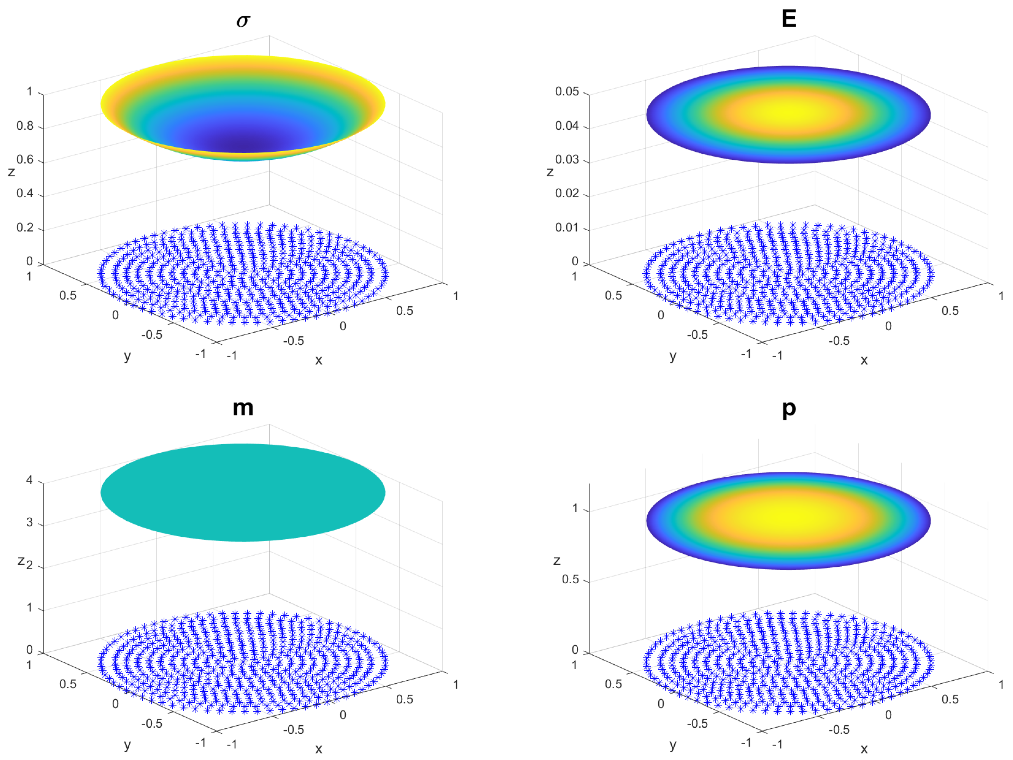
We solve numerically, using GFDM, system (5) with boundary conditions (27) and initial conditions (28) in the three discretised domains (clouds of points) represented in Figure 1. For each cloud of points and for time values of 2, 5 and 10 s, the graphs of the functions $\sigma$, E, m and p have been obtained. In all the graphs, the discretised domain has been represented in the $x-y$ plane and in the z-axis the values obtained for the previous mentioned functions, i.e., $\sigma$, E, m and p.

4.1. Example 1: Square

We plot in Figure 2, Figure 3 and Figure 4 the results obtained from the application of the GFDM to system (5) with the previous parameters for times $t=2,$ 5 and 10 s.

Figure 2. Graphs of the functions: $\sigma$, E, m and p for $t=2$ s.

Figure 3. Graphs of the functions: $\sigma$, E, m and p for $t=5$ s.

Figure 4. Graphs of the functions: $\sigma$, E, m and p for $t=10$ s.

4.2. Example 2: Circle (Regular)

Figure 5, Figure 6 and Figure 7 shows the numerical solutions given by the GFDM for times $t=2,$ 5 and 10 s.

Figure 5. Graphs of the functions: $\sigma$, E, m and p for $t=2$ s.

Figure 6. Graphs of the functions: $\sigma$, E, m and p for $t=5$ s.

Figure 7. Graphs of the functions: $\sigma$, E, m and p for $t=10$ s.

4.3. Example 3: Circle (Irregular)

Finally, we test the method using the third irregular cloud of Figure 1. We present in Figure 8, Figure 9 and Figure 10, for times $t=2,$ 5 and 10 s respectively, the plot of the discrete solution of system (5).

Figure 8. Graphs of the functions: $\sigma$, E, m and p for $t=2$ s.

Figure 9. Graphs of the functions: $\sigma$, E, m and p for $t=5$ s.

Figure 10. Graphs of the functions: $\sigma$, E, m and p for $t=10$ s.

5. Conclusions

We have propounded a meshless numerical scheme for the recently published model (1) in [8]. Convergence of the explicit formulae is obtained under some restrictions on the time step, $\mathsf{\Delta }t$, depending on the distribution of the nodes and the parameters of the problem. Finally, we have applied the method for solving three cases over regular and irregular domains, showing that the GFDM can be a powerful tool for implementing realistic examples of this important model of tumor growth.