Analysis, Evaluation and Exact Tracking of the Finite Precision Error Generated in Arbitrary Number of Multiplications

Abstract

In the present paper, a novel approach is introduced for the study, estimation and exact tracking of the finite precision error generated and accumulated during any number of multiplications. It is shown that, as a rule, this operation is very “toxic”, in the sense that it may force the finite precision error accumulation to grow arbitrarily large, under specific conditions that are fully described here. First, an ensemble of definitions of general applicability is given for the rigorous determination of the number of erroneous digits accumulated in any quantity of an arbitrary algorithm. Next, the exact number of erroneous digits produced in a single multiplication is given as a function of the involved operands, together with formulae offering the corresponding probabilities. In case the statistical properties of these operands are known, exact evaluation of the aforementioned probabilities takes place. Subsequently, the statistical properties of the accumulated finite precision error during any number of successive multiplications are explicitly analyzed. A method for exact tracking of this accumulated error is presented, together with associated theorems. Moreover, numerous dedicated experiments are developed and the corresponding results that fully support the theoretical analysis are given. Eventually, a number of important, probable and possible applications is proposed, where all of them are based on the methodology and the results introduced in the present work. The proposed methodology is expandable, so as to tackle the round-off error analysis in all arithmetic operations.

1. Introduction

All contemporary computing machines store both integer and floating-point numbers with a finite number of digits. This piece of fixed-sized data that is handled as a unity by the instruction set or the processor’s hardware is called finite word; the number of bits that form this piece of data, is frequently called “finite word length” or “employed precision”. In addition, on the hardware level, a computer performs fundamental operations, using a finite word length. Nowadays, dedicated software programs have been developed, which perform operations with a finite number of digits, the value of which is chosen by the programmer and/or the user, the only limitation being the memory and time constraints. We shall also use for this number of digits the term “finite word length” or “employed precision”.

Due to the fact that the precision with which all arithmetic operations are made is always limited, a numerical error is, as a rule, accumulated during the execution of most algorithms. In particular, in various algorithms and corresponding applications, the obtained results may be totally erroneous and/or unreliable due to the aforementioned reasons, which are inherent to all computing machines. We stress that this problem exists even when an arbitrarily large finite word length is employed for the execution of the algorithm, as it will become evident from the analysis introduced in the present paper. For this reason, we will use the term “finite precision error” for this numerical error; various authors and researchers also use the term “quantization error”, “round-off error” or other equivalent terms.

Consequently, a number of articles address the associated issues and the problems they generate. Thus, for example, authors in [1] study the finite precision error in the least mean square (LMS) adaptive algorithm and they show that the error’s mean squared value is inversely proportional to the adaptation step size μ. Reference [2] introduces a fast algorithm for exponentially weighted least squares Kalman filtering, which suffers less from finite precision error drawbacks, intrinsic to this class of algorithms. Reference [3] presents algorithms for accurately converting floating-point numbers to decimal representation. Article [4] studies the finite precision effects on the execution of the Lanczos algorithm for solving the standard non-symmetric eigenvalue problem. The authors of [5] study round-off error propagation in an algorithm which computes the orthonormal basis of a Krylov subspace with Householder orthonormal matrices. Authors in [6] study the propagation of round-off error near the periodic orbits of a discretized linear area-preserving map. The round-off error probability distribution, considered as a function of time, is shown to be a calculable algebraic number. In [7] it is shown that there are theoretically convergent schemes that solve non-linear partial differential equations, which can produce numerical steady state solutions that do not correspond to steady state solutions of the boundary value problem. In [8], it is pointed out that the convergence of Gegenbauer polynomials at the endpoints is affected by round-off error; the article proposes both parameter optimization and reduction of the round-off error for the Gegenbauer reconstruction method. In [9], a set of specific semantics is introduced which describes the propagation of round-off error during a calculation. The authors of [10] give an estimation of the round-off error generated in long-time integration in a number of standard, nonlinear systems. Authors in [11] introduce an algorithm for the computation of the orthogonal Fourier–Mellin moments which is of linear complexity and is resistant to finite precision error effects. Reference [12] proposes a method for dealing with the instability of the digital frequency synthesis (DFS), caused by the round-off error. Article [13] presents bounds for round-off error, generated in various algorithms. Moreover, another approach is presented in [14], according to which, the evolution of round-off error in chaotic maps is treated as an additive noise to the expected exact solutions; the introduced method spots a threshold below which global errors may be ignored. Article [15] studies the round-off error generated during computation of Hardy’s multiquadric and its related interpolators and proposes the use of arbitrary precision arithmetics to circumvent the associated finite precision error problems. Authors of [16] propose a fast, resistant to finite precision error method for evaluation of high order Zernike moments. Article [17] proposes a method for an improved scaling of finite precision error analysis. Finally, in [18,19], a preliminary form of the approach introduced here is presented.

In the present paper, we introduce a novel approach for studying and evaluating the finite precision error generated during the operation of multiplication. It is shown that, as a rule, this operation is very “toxic”, in the sense that it may force the finite precision error accumulation to grow arbitrarily large. The exact amount of the generated number of erroneous digits added or subtracted to the result (product) of this operation is given. Consequently, the probabilities the number of erroneous digits of the product differ by k from the maximum number of erroneous digits of the operands are explicitly computed. In the process of doing so, a set of general definitions is given, applicable to all operations performed with finite word length by a computing machine. Then, the accumulation of erroneous digits after an arbitrary number of successive multiplications is extensively analyzed. Statistical properties of this accumulated error are stated that allow for exact error prediction when the distribution of the associated operands are given. In addition, a number of theoretical results are introduced, which allow for the exact tracking of the generated and accumulated finite precision error during any number of multiplications in general. Numerous experimental results are presented, which fully support the presented theoretical analysis. We stress that the introduced methodology is expandable, so as to tackle all arithmetic operations.

2. A Set of Basic Definitions, Notations and Abbreviations

The entire analysis will be mainly made in the decimal arithmetic system, only because this system is far more familiar to most users. However, all results referred to in the present work hold perfectly well for the binary system too, or any other radix; the corresponding analysis and deductions may be obtained by means of a quite straightforward and slight modification of the approach introduced here.

In any arithmetic system, we assume that all numbers are expressed in scientific/canonical form. Thus, any number $x$ is written as $mantissa·{10}^{\tau }$, in the decimal arithmetic system, where $\left|mantissa\right|\in \left[1,\left.10\right), \tau \in \mathbb{Z}\right.$; in the binary system, the same number is expressed as $mantissa·2^{\tau }$, where $\left|mantissa\right|\in \left[1,\left.2\right), \tau \in \mathbb{Z}\right.$. Independently of the employed radix, we will use the symbols $man\left(x\right)$ and $E\left(x\right)$ for the mantissa and the exponent of any quantity $x$ respectively. We shall demonstrate in the following that the analysis introduced here based on the decimal radix offers accurate results and prediction for the multiplication(s) performed by computing machines.

Abbreviations 1.

We will use the acronym e. d. d. in place of “erroneous decimal digits” and c. d. d. for “correct decimal digits”. In general, abbreviation “d. d.” stands for “decimal digits”. The abbreviation f. p. e. stands for “finite precision error”. The symbols$\#edd\left(x\right)$and$\#cdd\left(x\right)$stand for the number of e. d. d. accumulated in quantity$x$, due to f. p. e., and its number of c. d. d. respectively.

Notation 1.

The expressions the algorithm “has failed” or it “has been destroyed due to f. p. e.” mean that the algorithm in hand offers completely unreliable results, at a certain iteration.

Suppose that any two numbers $\alpha$ and $\beta$ are given, both written in canonical form. In order to unambiguously verify if these two numbers share a common number of initial digits (i.e., stem of digits), starting from the most significant one, we shall employ the following:

Definition 1.

Consider two numbers,$\alpha ,\beta$of the same sign, written in scientific form, with the same number,$n$, of decimal digits in the mantissa:

$$\alpha =man\left(\alpha \right)·{10}^{\tau },\beta =man\left(\beta \right)·{10}^{\rho }$$

where$\tau ={\rm E}\left(\alpha \right)$and$\rho ={\rm E}\left(\beta \right)$. Let us assume, without any loss of generality, that$\tau \ge \rho$holds. Then, these two numbers share the first$\mu ,\mu \in \mathbb{N}$digits (they have the first$\mu$digits in common) if and only if:

$$\left|\alpha -\beta \right|=w·{10}^{\tau -\mu },w\in \left[1,\right.\left.10\right).$$

Consequently,$\alpha$and$\beta$differ in the last$\lambda ,\lambda \in \mathbb{N}$digits if and only if:

$$\left|\alpha -\beta \right|=z·{10}^{\tau -\left(n-\lambda \right)},z\in \left[1,\right.\left.10\right).$$

(2.1)

Evidently, in the binary system, the two numbers share the first$\mu ,\mu \in \mathbb{N}$bits if and only if

$$\left|\alpha -\beta \right|=w·2^{E\left(\alpha \right)-\mu },w\in \left[1,\right.\left.2\right),$$

(2.2)

where$n$is the finite word length, while they differ in the last$\lambda ,\lambda \in \mathbb{N}$digits if and only if

$$\left|\alpha -\beta \right|=z·2^{E\left(a\right)-\left(n-\lambda \right)},z\in \left[1,\right.\left.2\right).$$

(2.3)

If the aforementioned relation offers a negative$\lambda$, then, by definition,$\lambda =0$, namely$\alpha$and$\beta$are identical as far as all their$n$digits are concerned.

Now, we shall give a couple of examples in order to clarify the content of Definition 1.

Example 1.

$$n_1=4.269587962\mathbf{400597}·{10}^4$$

$$n_2=4.269587962\mathbf{393951}·{10}^4$$

A simple inspection might lead someone to deduce that these two numbers differ by six (6) decimal digits. Actually and according to Definition 1, the following holds:

$$\tau =\rho =4$$

$$n=16$$

where the absolute difference is$\left|n_1-n_2\right|=6.6459·{10}^{-8}$

Hence,

$$\tau -\left(n-k\right)=-8\iff k=4$$

Therefore, the two aforementioned numbers differ in four (4) decimal digits, contrary to a probable initial expectation.

Example 2.

According to Definition 1, the two numbers with 32 decimal digits in the mantissa,

$$n_1=6.98765432123456789\mathbf{77777777777777}·{10}^1,$$

$$n_2=6.98765432123456789\mathbf{01523451234533}·{10}^1,$$

differ by 14 decimal digits, shown in bold, since$\tau =\rho =1,n=32$, while their absolute difference is$\left|n_1-n_2\right|=7.6254326543244·{10}^{-17}$; hence,$\tau -\left(n-k\right)=-5\iff k=14$.

Additionally, the two numbers$n_1=1.112324567422342·{10}^4$and$n_2=1.112324567421112·{10}^4$differ by 4 decimal digits in the mantissa, since$\tau =\rho =4,n=16$and$\left|n_1-n_2\right|=1.230000634677708·{10}^{-8}$; therefore,$\tau -\left(n-k\right)=-8\iff k=4$.

Similarly, the two numbers$n_1=1.00000000·{10}^{\tau }$and$n_2=9.99999999·{10}^{\tau -1}$do not differ at all, since$\left|n_1-n_2\right|=9.999999717180685·{10}^{-10}$; hence$\tau -\left(n-k\right)=-10\iff k=-1-\tau <0.$

Suppose, moreover, that all operations were made with infinite precision; then, let an arbitrary quantity $\alpha$ have the value ${\tilde{a}}^c$, where superscript $c$ indicates the ideally correct value of $\alpha$. Next, suppose that the very same quantity $\alpha$ is calculated in a computing machine which performs the same operations as in the infinite case, using $n$ digits in the mantissa; suppose that this machine generates the representation ${\alpha }_n$ for the specific quantity $a$. Then, a rigorous relation between ${\alpha }_n$ and ${\tilde{a}}^c$ is obtained via the following:

Definition 2.

Let us assume that we restrict the infinite precision quantity${\tilde{a}}^c$to its first$n$digits, obtaining quantity$a^c$. Let us also assume that comparison of${\alpha }_n$and$a^c$by means of Definition 1, manifests that these two quantities differ by${\lambda }_{\alpha }$digits. Then, we deduce that quantity${\alpha }_n$has the first${\lambda }_c=\left(n-{\lambda }_{\alpha }\right)$digits correct and all its other digits erroneous. The aforementioned statement holds for both the binary system, which is the base of contemporary computing machines, as well as for the decimal radix.

A number of practical examples associated with the above Definition, will be given in Section 6.

It is known that a mantissa represented by a number of bits, say $\nu , \nu \in \mathbb{N}$, in a computing machine is approximated in the decimal radix by a number $n$ of d. d., pretty close to the nearest integer of $\nu ·{log}_{10}2$. Since $\nu ·{log}_{10}2$ is, as a rule, not an integer, then the number of correct digits of a quantity’s decimal representation may fluctuate by one digit at most.

3. Generation of Finite Precision Error in a Single Multiplication and Corresponding Probabilities

This Section presents a solution to the following problem: consider two arbitrary numbers, say ${\alpha }_n$, ${\beta }_n$ found in a computing machine that uses a finite word length of $n$ decimal digits in the mantissa. Moreover, suppose due to an ensemble of previous calculations ${\alpha }_n$ has been computed with ${\lambda }_{\alpha }$ erroneous decimal digits (e. d. d.) in its mantissa, while ${\beta }_n$ with ${\lambda }_{\beta }$ e. d. d. in the mantissa. In addition, consider that multiplication ${\gamma }_n={\alpha }_n{\beta }_n$ is executed in this computing machine. Then, so far, it has been an open question to determine the exact number of e. d. d. with which ${\gamma }_n$ is evaluated; moreover, the corresponding probabilities that ${\gamma }_n$ is computed with a specific number of e. d. d. must be evaluated.

3.1. Bounds and Evaluation of the Finite Precision Error Produced in a Single Multiplication

Consider any two quantities $\alpha ,\beta$ having ${\tilde{a}}^c \mathrm{and} {\tilde{\beta }}^c$ ideally correct digits, should all operations and representations be made with infinite precision. Next, suppose that quantities $\alpha$ and $\beta$ have been evaluated in a computing machine using $n$ d. d. in the mantissa; we let the representations of these two numbers in this computing machine be $a_n$ and ${\beta }_n$, respectively. In addition, following Definition 2, we let the restriction of ${\tilde{a}}^c \mathrm{and} {\tilde{\beta }}^c$ in this machine be ${\alpha }^c,{\beta }^c$ respectively. We would like to emphasize that the difference between $a_n$ and $a^c$ is the following: quantity ${\alpha }_n$ may have been evaluated with finite precision error, due to previous calculations. On the contrary, $a^c$ is free of finite precision error since it is always considered to be a restriction of the ideally correct value of ${\tilde{a}}^c$ in $n$ decimal digits.

Consider, moreover, the product $\gamma =\alpha ·\beta$, executed both with infinite precision yielding product ${\gamma }^c={\alpha }^c·{\beta }^c$, as well as in a computing machine using $n$ digits in the mantissa, generating ${\gamma }_n={\alpha }_n·{\beta }_n$. In addition, suppose that, due to previous calculations, ${\alpha }_n$ has been computed with ${\lambda }_{\alpha }$ erroneous decimal digits (e. d. d.), ($\iff {\lambda }_a^c=n-{\lambda }_{\alpha }$ correct decimal digits), while ${\beta }_n$ with ${\lambda }_{\beta }$ e. d. d. ($\iff$ ${\lambda }_{\beta }^c=n-{\lambda }_{\beta }$ c. d. d.) due to the fact that all operations have been made with a finite word length. We note, as it will become evident in the following analysis, that the finite precision error generated in the multiplication process is located only in the mantissae of the involved terms. Hence, we may assume that ${\alpha }_n$, ${\beta }_n$, ${\alpha }^c$ and ${\beta }^c$ are plain mantissae, namely that $E\left({\alpha }_n\right)={\rm E}\left({\beta }_n\right)=\tau =0$. In order to study the finite precision error generated in the computation of the product $\gamma$, we distinguish a number of cases, which are analytically presented below; in addition, a concise presentation of all these cases takes place in Table 1 and Table 2, positioned in the end of the present sub-section. Thus:

Table 1. This refers to Case 1, with ${\lambda }_{\alpha }^c={\lambda }_{\beta }^c={\lambda }^c$. The first column under the title “sub-cases”, the eventual values of $M_1=\left|{\alpha }_{n}x+{\beta }_{n}y\right|$ are shown. In Line 3, in the right of the same title, the possible values of the product $\left|man\left({\alpha }_n\right)man\left({\beta }_n\right)\right|$ are presented. The obtained number of correct decimal digits (c. d. d.) of product ${\gamma }_n=a_n{\beta }_n$ is shown in bold in each corresponding square.

$\mathbf{Case}\mathbf{1}\mathbf{:}\mathbf{Number}\mathbf{of}\mathbf{c}\mathbf{.}\mathbf{d}\mathbf{.}\mathbf{d}\mathbf{.}\mathbf{of}\mathbf{Product}{\mathit{\gamma }}_{\mathit{n}}$$\mathbf{When}{\mathit{\lambda }}_{\mathit{\alpha }}^{\mathit{c}}\mathbf{=}{\mathit{\lambda }}_{\mathit{\beta }}^{\mathit{c}}\mathbf{=}{\mathit{\lambda }}^{\mathit{c}}\mathbf{.}$
$\mathbf{Let}{\mathit{M}}_{\mathbf{1}}\mathbf{=}\left|{\mathit{\alpha }}_{\mathit{n}}\mathit{x}\mathbf{+}{\mathit{\beta }}_{\mathit{n}}\mathit{y}\right|\mathbf{.}$
Sub-Cases	$\mathbf{(}\mathbf{1}\mathbf{.}\mathbf{i}\mathbf{)}\left|\mathit{m}\mathit{a}\mathit{n}\left({\mathit{\alpha }}_{\mathit{n}}\right)\mathit{m}\mathit{a}\mathit{n}\left({\mathit{\beta }}_{\mathit{n}}\right)\right|\mathbf{<}\mathbf{10}$	$\mathbf{(}\mathbf{1}\mathbf{.}\mathbf{ii}\mathbf{)}\left|\mathit{m}\mathit{a}\mathit{n}\left({\mathit{\alpha }}_{\mathit{n}}\right)\mathit{m}\mathit{a}\mathit{n}\left({\mathit{\beta }}_{\mathit{n}}\right)\right|\mathbf{\ge }\mathbf{10}$
(a)$100\le M_1<\mathrm{UB}$	${\lambda }^c-2$	${\lambda }^c-1$
(b)$10\le M_1<100$	${\lambda }^c-1$	${\lambda }^c$
(c)$1\le M_1<10$	${\lambda }^c$	${\lambda }^c+1$
(d)${10}^{-1}\le M_1<1$	${\lambda }^c+1$	${\lambda }^c+2$
(e)${10}^{-k}\le M_1<{10}^{-\left(k-1\right)},$ $k=2,3,4$	${\lambda }^c+k$	${\lambda }^c+k+1$

Table 2. It refers to Case 2, where ${\lambda }_{\alpha }^c\ne {\lambda }_{\beta }^c$ and in particular ${\lambda }_{\alpha }^c>{\lambda }_{\beta }^c$, without any loss of generality. The first column under the title “sub-cases”, the eventual values of $M_2=\left|{\alpha }_{n}x+{\beta }_{n}y·{10}^{-\left({\lambda }_a^c-{\lambda }_{\beta }^c\right)}\right|$ are shown. In Line 3, in the right of the same title, the possible values of the product $\left|man\left({\alpha }_n\right)man\left({\beta }_n\right)\right|$ are presented. The obtained number of correct decimal digits (c. d. d.) of product ${\gamma }_n=a_n{\beta }_n$ is shown in bold in each corresponding square.

$\mathbf{Case}\mathbf{2}\mathbf{:}\mathbf{Number}\mathbf{of}\mathbf{c}\mathbf{.}\mathbf{d}\mathbf{.}\mathbf{d}\mathbf{.}\mathbf{of}\mathbf{Product}{\mathit{\gamma }}_{\mathit{n}}$$\mathbf{When}{\mathit{\lambda }}_{\mathit{\alpha }}^{\mathit{c}}\mathbf{>}{\mathit{\lambda }}_{\mathit{\beta }}^{\mathit{c}}\mathbf{.}$
$\mathbf{Let}{\mathit{M}}_{\mathbf{2}}\mathbf{=}\left|{\mathit{\alpha }}_{\mathit{n}}\mathit{x}\mathbf{+}{\mathit{\beta }}_{\mathit{n}}\mathit{y}\mathbf{·}{\mathbf{10}}^{\mathbf{-}\left({\mathit{\lambda }}_{\mathit{a}}^{\mathit{c}}\mathbf{-}{\mathit{\lambda }}_{\mathit{\beta }}^{\mathit{c}}\right)}\right|.$
Sub-Cases	$\mathbf{(}\mathbf{2}\mathbf{.}\mathbf{i}\mathbf{)}\left|\mathit{m}\mathit{a}\mathit{n}\left({\mathit{\alpha }}_{\mathit{n}}\right)\mathit{m}\mathit{a}\mathit{n}\left({\mathit{\beta }}_{\mathit{n}}\right)\right|\mathbf{<}\mathbf{10}$	$\mathbf{(}\mathbf{2}\mathbf{.}\mathbf{ii}\mathbf{)}\left|\mathit{m}\mathit{a}\mathit{n}\left({\mathit{\alpha }}_{\mathit{n}}\right)\mathit{m}\mathit{a}\mathit{n}\left({\mathit{\beta }}_{\mathit{n}}\right)\right|\mathbf{\ge }\mathbf{10}$
(a)$100\le M_1$	${\lambda }_{\beta }^c-2$	${\lambda }_{\beta }^c-1$
(b)$10\le M_1<100$	${\lambda }_{\beta }^c-1$	${\lambda }_{\beta }^c$
(c)$1\le M_1<10$	${\lambda }_{\beta }^c$	${\lambda }_{\beta }^c+1$
(d)${10}^{-1}\le M_1<1$	${\lambda }_{\beta }^c+1$	${\lambda }_{\beta }^c+2$
(e)${10}^{-k}\le M_1<{10}^{-\left(k-1\right)},$ $k=2,3,4$	${\lambda }_{\beta }^c+k$	${\lambda }_{\beta }^c+k+1$

Case 1. Quantities ${\alpha }_n$ and ${\beta }_n$ share the same number of correct decimal digits $\left({\lambda }_a^c={\lambda }_{\beta }^c\right)$.

Therefore, according to Definition 2, it holds that

$$\left|{\alpha }_n-a^c\right|=z·{10}^{0-\left(n-{\lambda }_a\right)},z\in \left[1,\right.\left.10\right),$$

from which we deduce that we can express quantities ${\alpha }^c$ and ${\beta }^c$ as follows:

$${\alpha }^c={\alpha }_n+y·{10}^{-{\lambda }_a^c}{\beta }^c={\beta }_n+x·{10}^{-{\lambda }_{\beta }^c},$$

(3.1)

where $x$ and $y$ are the signed mantissae of the finite precision error. Taking (3.1) into consideration, we may write:

$${\gamma }^c={\alpha }^c·{\beta }^c\stackrel{\left(3.1\right)}{=}{\alpha }_n{\beta }_n+{\alpha }_{n}x·{10}^{-{\lambda }_{\beta }^c}+{\beta }_{n}y·{10}^{-{\lambda }_a^c}+xy·{10}^{-\left({\lambda }_a^c+{\lambda }_{\beta }^c\right)}.$$

Since, by hypothesis, ${\lambda }_a^c={\lambda }_{\beta }^c={\lambda }^c$, the above expression becomes

$${\gamma }^c={\alpha }_n{\beta }_n+\left({\alpha }_{n}x+{\beta }_{n}y\right)·{10}^{-{\lambda }^c}+xy·{10}^{-2{\lambda }^c}$$

(3.2)

Thus, according to Definition 2, the finite precision error (f. p. e.) with which product ${\gamma }_n$ has been evaluated is

$${\epsilon }_{\gamma }=\left({\alpha }_{n}x+{\beta }_{n}y\right)·{10}^{-{\lambda }^c}+xy·{10}^{-2{\lambda }^c}.$$

(3.3)

We point out that the subsequent analysis may use (3.3) with slight, straightforward modifications; in fact, in practice, it is sufficient to keep the first-order terms when ${\lambda }^c\ge 3$, since term $xy·{10}^{-2{\lambda }^c}$ is practically negligible. Should the algorithm tend to fail, i.e., if ${\lambda }^c<3$, then, ${\epsilon }_{\gamma }$ of (3.3) can be used in the subsequent analysis, in a very straightforward manner. To compute the number of erroneous decimal digits (e. d. d.) of ${\gamma }_n$, it is absolutely necessary to distinguish the cases $\left|man\left({\alpha }_n\right)man\left({\beta }_n\right)\right|<10$ and $\left|man\left({\alpha }_n\right)man\left({\beta }_n\right)\right|\ge 10$, for reasons that will become evident in the following. In fact:

Case 1.i. It refers to inequality

$$\left|man\left({\alpha }_n\right)man\left({\beta }_n\right)\right|<10.$$

(3.4)

Immediately below we will show that, in this case, the maximum number of additional erroneous decimal digits generated in the multiplication ${\gamma }_n={\alpha }_n·{\beta }_n$ is 2. Indeed, here, since we have assumed that all involved quantities have zero exponents, the product ${\alpha }_n{\beta }_n$, is given by ${\alpha }_n{\beta }_n=man\left({\alpha }_n\right)man\left({\beta }_n\right)=man\left({\alpha }_n{\beta }_n\right)$; now, (3.2) becomes

$${\gamma }^c={\alpha }^c{\beta }^c=man\left({\alpha }_n{\beta }_n\right)+\left({\alpha }_{n}x+{\beta }_{n}y\right)·{10}^{-{\lambda }^c}$$

(3.5)

using the aforementioned first-order approximation. Hence, given that $\left|man\left({\alpha }_n\right)man\left({\beta }_n\right)\right|<10$, it is rather straightforward to show that the supremum of quantity $\left|{\alpha }_{n}x+{\beta }_{n}y\right|$ may acquire is $UB=110$, since all terms, ${\alpha }_n,{\beta }_n,x,y$, are mantissae. Therefore, we distinguish the following sub-cases:

Case 1.i.a:

$$100\le \left|{\alpha }_{n}x+{\beta }_{n}y\right|<UB.$$

(3.6)

Then, ${\alpha }_{n}x+{\beta }_{n}y=man\left({\alpha }_{n}x+{\beta }_{n}y\right)·{10}^2$, which implies that

$$man\left({\alpha }^c{\beta }^c\right)=man\left({\alpha }_n{\beta }_n\right)+man\left({\alpha }_{n}x+{\beta }_{n}y\right)·{10}^{-\left({\lambda }^c-2\right)}.$$

(3.7)

The above relation (3.7) implies that

$$\left|man\left({\alpha }^c{\beta }^c\right)-man\left({\alpha }_n{\beta }_n\right)\right|=\left|man\left({\alpha }_{n}x+{\beta }_{n}y\right)\right|·{10}^{-\left({\lambda }^c-2\right)},$$

Which according to Definition 2 shows that quantity ${\gamma }_n={\alpha }_n{\beta }_n$ has been computed with two less correct decimal digits, namely with $\left({\lambda }^c-2\right)$ correct decimal digits (c. d. d.) or equivalently with two additional erroneous decimal digits than those of the operands ${\alpha }_n$ and ${\beta }_n$.

Case 1.i.b:

$$10\le \left|{\alpha }_{n}x+{\beta }_{n}y\right|<100.$$

(3.8)

In this sub-case, ${\alpha }_{n}x+{\beta }_{n}y=man\left({\alpha }_{n}x+{\beta }_{n}y\right)·10$, which implies that

$${\gamma }^c=man\left({\alpha }_n{\beta }_n\right)+man\left({\alpha }_{n}x+{\beta }_{n}y\right)·{10}^{-\left({\lambda }^c-1\right)}.$$

(3.9)

Consequently, Definition 2, implies that ${\gamma }_n$ has been computed with one less c. d. d. than ${\alpha }_n$ and ${\beta }_n$.

Case 1.i.c:

$$1\le \left|{\alpha }_{n}x+{\beta }_{n}y\right|<10.$$

(3.10)

Now, ${\alpha }_{n}x+{\beta }_{n}y=man\left({\alpha }_{n}x+{\beta }_{n}y\right)$, implying that

$${\gamma }^c=man\left({\alpha }_n{\beta }_n\right)+man\left({\alpha }_{n}x+{\beta }_{n}y\right)·{10}^{-{\lambda }^c}.$$

(3.11)

Together with Definition 2, this means that ${\gamma }_n$ has the same number of c. d. d. with ${\alpha }_n$ and ${\beta }_n$, namely ${\lambda }^c$.

Case 1.i.d:

$${10}^{-1}\le \left|{\alpha }_{n}x+{\beta }_{n}y\right|<1.$$

(3.12)

Here it holds that ${\alpha }_{n}x+{\beta }_{n}y=man\left({\alpha }_{n}x+{\beta }_{n}y\right)·{10}^{-1}$, implying that

$${\gamma }^c=man\left({\alpha }_n{\beta }_n\right)+man\left({\alpha }_{n}x+{\beta }_{n}y\right)·{10}^{-\left({\lambda }^c+1\right)}.$$

(3.13)

Consequently, one may deduce that the number of ${\gamma }_n$’s erroneous decimal digits (e. d. d.) has been reduced by one.

Case 1.i.e. This constitutes a generalization of Case 1.i.d.; in fact, now, we assume that the following inequality holds:

$${10}^{-k}\le \left|{\alpha }_{n}x+{\beta }_{n}y\right|<{10}^{-\left(k-1\right)},k=2,3,4.$$

(3.14)

In this, more general case, it holds that ${\alpha }_{n}x+{\beta }_{n}y=man\left({\alpha }_{n}x+{\beta }_{n}y\right)·{10}^{-k}$, therefore,

$${\gamma }^c=man\left({\alpha }_n{\beta }_n\right)+man\left({\alpha }_{n}x+{\beta }_{n}y\right)·{10}^{-\left({\lambda }^c+k\right)}.$$

(3.15)

Hence, the number of correct decimal digits (c. d. d.) of ${\gamma }_n$ has been increased by $k$. The same approach may be applied for $k\ge 5$; however, we will show that the corresponding probabilities are negligible in practice.

Case 1.ii, which concerns inequality

$$\left|man\left({\alpha }_n\right)man\left({\beta }_n\right)\right|\ge 10.$$

(3.16)

Since ${\alpha }_n, {\beta }_n, x, y$ are mantissae, $\left|{\alpha }_{n}x+{\beta }_{n}y\right|<200$ holds. Therefore, we distinguish the following cases:

Case 1.ii.a:

$$100\le \left|{\alpha }_{n}x+{\beta }_{n}y\right|<200.$$

(3.17)

In this case, ${\alpha }_{n}x+{\beta }_{n}y=man\left({\alpha }_{n}x+{\beta }_{n}y\right)·{10}^2$, which implies that

$${\gamma }^c=man\left({\alpha }_n{\beta }_n\right)+man\left({\alpha }_{n}x+{\beta }_{n}y\right)·{10}^{-\left({\lambda }^c-2\right)}.$$

(3.18)

However, ${\alpha }_n{\beta }_n=man\left({\alpha }_n\right)man\left({\beta }_n\right)=man\left({\alpha }_n{\beta }_n\right)·10\Rightarrow {\alpha }^c{\beta }^c=man\left({\alpha }^c{\beta }^c\right)·10$, if the algorithm has not failed, which means that $E\left({\alpha }^c{\beta }^c\right)=E\left({\alpha }_n{\beta }_n\right)$. Thus, (3.18) now reads:

$$\begin{gathered} {\gamma }^c={\alpha }^c{\beta }^c=man\left({\alpha }^c{\beta }^c\right)·10=man\left({\alpha }_n{\beta }_n\right)·10+\left({\alpha }_{n}x+{\beta }_{n}y\right)·{10}^{-{\lambda }^c} \\ =man\left({\alpha }_n{\beta }_n\right)·10+man\left({\alpha }_{n}x+{\beta }_{n}y\right)·{10}^2·{10}^{-{\lambda }^c}\iff \\ man\left({\alpha }^c{\beta }^c\right)=man\left({\alpha }_n{\beta }_n\right)+man\left({\alpha }_{n}x+{\beta }_{n}y\right)·{10}^{-\left({\lambda }^c-1\right)}\Rightarrow \\ \left|man\left({\alpha }^c{\beta }^c\right)-man\left({\alpha }_n{\beta }_n\right)\right|=\left|man\left({\alpha }_{n}x+{\beta }_{n}y\right)\right|·{10}^{-\left({\lambda }^c-1\right)}. \end{gathered}$$

(3.19)

The above equality (3.19), together with Definition 2 dictates that ${\gamma }_n$ has been evaluated with $\left({\lambda }^c-1\right)$ correct decimal digits (c. d. d.). Even though (3.6) and (3.17) are quite similar, now, the number of erroneous decimal digits (e. d. d.) of ${\gamma }_n$ has been reduced by one, due to the right shift the computing machine has performed, to represent ${\gamma }_n$ in its canonical form.

Case 1.ii.b:

$$10\le \left|{\alpha }_{n}x+{\beta }_{n}y\right|<100.$$

(3.20)

In this case, ${\alpha }_{n}x+{\beta }_{n}y=man\left({\alpha }_{n}x+{\beta }_{n}y\right)·10$ holds. However, now, once more, provided that the algorithm has not failed, one obtains ${\alpha }_n{\beta }_n=man\left({\alpha }_n{\beta }_n\right)·10$ and ${\alpha }^c{\beta }^c=man\left({\alpha }^c{\beta }^c\right)·10.$ Hence,

$$\begin{gathered} {\gamma }^c={\alpha }^c{\beta }^c=man\left({\alpha }^c{\beta }^c\right)\cdot 10=\left(man\left({\alpha }_n{\beta }_n\right)+man\left({\alpha }_{n}x+{\beta }_{n}y\right)·{10}^{-{\lambda }^c}\right)·10 \\ \iff man\left({\alpha }^c{\beta }^c\right)=man\left({\alpha }_n{\beta }_n\right)+man\left({\alpha }_{n}x+{\beta }_{n}y\right)·{10}^{-{\lambda }^c}. \end{gathered}$$

(3.21)

Definition 2 indicates that ${\gamma }_n$ has been evaluated with ${\lambda }^c$ c. d. d. (i.e., with no additional finite precision error (f. p. e.)).

Case 1.ii.c:

$$1\le \left|{\alpha }_{n}x+{\beta }_{n}y\right|<10.$$

(3.22)

Now it holds that ${\alpha }_{n}x+{\beta }_{n}y=man\left({\alpha }_{n}x+{\beta }_{n}y\right)$. Supposing that the algorithm has not failed, one deduces

$$\begin{gathered} {\gamma }^c={\alpha }^c{\beta }^c=man\left({\alpha }^c{\beta }^c\right)·10=man\left({\alpha }_n{\beta }_n\right)·10+man\left({\alpha }_{n}x+{\beta }_{n}y\right)·{10}^{-{\lambda }^c} \\ \iff man\left({\alpha }^c{\beta }^c\right)=man\left({\alpha }_n{\beta }_n\right)+man\left({\alpha }_{n}x+{\beta }_{n}y\right)·{10}^{-\left({\lambda }^c+1\right)}\Rightarrow \\ \left|man\left({\alpha }^c{\beta }^c\right)-man\left({\alpha }_n{\beta }_n\right)\right|=\left|man\left({\alpha }_{n}x+{\beta }_{n}y\right)\right|·{10}^{-\left({\lambda }^c+1\right)}. \end{gathered}$$

(3.23)

The later implies that quantity ${\alpha }_n{\beta }_n$ has been computed with an additional correct decimal digit, i.e., that the multiplication operation has relaxed the finite precision error (f. p. e.) by one decimal digit.

Case 1.ii.d:

$${10}^{-k}\le \left|{\alpha }_{n}x+{\beta }_{n}y\right|<{10}^{-\left(k-1\right)},k=1,2,3,4.$$

(3.24)

In this case, it holds that ${\alpha }_{n}x+{\beta }_{n}y=man\left({\alpha }_{n}x+{\beta }_{n}y\right)·{10}^{-k}$, hence,

$$\begin{gathered} {\gamma }^c=man\left({\alpha }^c{\beta }^c\right)·10=man\left({\alpha }_n{\beta }_n\right)·10+man\left({\alpha }_{n}x+{\beta }_{n}y\right)·{10}^{-\left({\lambda }^c+k\right)}\iff \\ man\left({\alpha }^c{\beta }^c\right)=man\left({\alpha }_n{\beta }_n\right)+man\left({\alpha }_{n}x+{\beta }_{n}y\right)·{10}^{-\left({\lambda }^c+k+1\right)}. \end{gathered}$$

(3.25)

Consequently, the number of correct decimal digits (c. d. d.) of product ${\gamma }_n$ has been increased by $k+1$ in this case.

Case 2. ${\alpha }_n$ and ${\beta }_n$ have been calculated with different number of correct decimal digits $\left({\lambda }_a^c\ne {\lambda }_{\beta }^c·{\lambda }_{\alpha }\ne {\lambda }_{\beta }\right)$ Without any loss of generality, we may assume that ${\lambda }_{\alpha }⟨{\lambda }_{\beta }\iff {\lambda }_a^c⟩{\lambda }_{\beta }^c$. Consequently, once more it holds that:

$$\begin{gathered} {\alpha }^c={\alpha }_n+y·{10}^{-{\lambda }_a^c}{\beta }^c={\beta }_n+x·{10}^{-{\lambda }_{\beta }^c}\Rightarrow \\ {\gamma }^c={\alpha }^c·{\beta }^c={\alpha }_n{\beta }_n+{\alpha }_{n}x·{10}^{-{\lambda }_{\beta }^c}+{\beta }_{n}y·{10}^{-{\lambda }_a^c}+xy·{10}^{-\left({\lambda }_a^c+{\lambda }_{\beta }^c\right)}. \end{gathered}$$

(3.26)

As in Case 1, we will use a first-order approximation in (3.26).

Again, the introduced analysis may be extended in a straightforward manner to incorporate the higher order term, too; however, as it will become clear from the subsequent sections, the accuracy improvement is negligible, given also the dramatic increase in complexity. Thus, we may safely assume that ${\gamma }^c={\alpha }_n{\beta }_n+{\alpha }_{n}x·{10}^{-{\lambda }_{\beta }^c}+{\beta }_{n}y·{10}^{-{\lambda }_a^c}·{\alpha }^c{\beta }^c={\alpha }_n{\beta }_n+\left({\alpha }_{n}x+{\beta }_{n}y·{10}^{-\left({\lambda }_a^c-{\lambda }_{\beta }^c\right)}\right)·{10}^{-{\lambda }_{\beta }^c}$. After setting $\delta ={\lambda }_a^c-{\lambda }_{\beta }^c\ge 1$, we obtain:

$${\alpha }^c{\beta }^c={\alpha }_n{\beta }_n+\left({\alpha }_{n}x+{\beta }_{n}y·{10}^{-\delta }\right)·{10}^{-{\lambda }_{\beta }^c}.$$

(3.27)

We must now repeat the analysis previously made in connection with Case 1, by letting $\left({\alpha }_{n}x+{\beta }_{n}y·{10}^{-\delta }\right)$ play the role of ${\alpha }_{n}x+{\beta }_{n}y$ and ${\lambda }_{\beta }^c$ play the role of ${\lambda }^c$. Hence, we again distinguish the cases $\left|man\left({\alpha }_n\right)man\left({\beta }_n\right)\right|<10$ and $\left|man\left({\alpha }_n\right)man\left({\beta }_n\right)\right|\ge 10$, thus getting:

Case 2.i:$\left|man\left({\alpha }_n\right)man\left({\beta }_n\right)\right|<10$

Case 2.i.a:

$$100\le \left|{\alpha }_{n}x+{\beta }_{n}y·{10}^{-\delta }\right|.$$

(3.28)

In this case, $man\left({\alpha }^c{\beta }^c\right)=man\left({\alpha }_n{\beta }_n\right)+man\left({\alpha }_{n}x+{\beta }_{n}y·{10}^{-\delta }\right)·{10}^{-\left({\lambda }_{\beta }^c-2\right)}$.

Namely, product ${\gamma }_n$ is computed with two additional erroneous decimal digits (e. d. d.) than ${\lambda }_{\beta }$.

Case 2.i.b:

$$10\le \left|{\alpha }_{n}x+{\beta }_{n}y·{10}^{-\delta }\right|<100.$$

(3.29)

Now $man\left({\alpha }^c{\beta }^c\right)=man\left({\alpha }_n{\beta }_n\right)+man\left({\alpha }_{n}x+{\beta }_{n}y·{10}^{-\delta }\right)·{10}^{-\left({\lambda }_{\beta }^c-1\right)}$ which means that product ${\gamma }_n$ is calculated with one additional erroneous decimal digits (e. d. d.) than ${\beta }_n$.

Case 2.i.c:

$$1\le \left|{\alpha }_{n}x+{\beta }_{n}y·{10}^{-\delta }\right|<10.$$

(3.30)

Here, it holds that $man\left({\alpha }^c{\beta }^c\right)=man\left({\alpha }_n{\beta }_n\right)+man\left({\alpha }_{n}x+{\beta }_{n}y·{10}^{-\delta }\right)·{10}^{-{\lambda }_{\beta }^c}$.

Hence, product ${\gamma }_n$ is calculated with no additional e. d. d. when compared to ${\beta }_n$, namely ${\lambda }_{\beta }$.

Case 2.i.d:

$${10}^{-k}\le \left|{\alpha }_{n}x+{\beta }_{n}y·{10}^{-\delta }\right|<{10}^{-\left(k-1\right)},k=1,2,3.$$

(3.31)

In this case, $man\left({\alpha }^c{\beta }^c\right)=man\left({\alpha }_n{\beta }_n\right)+man\left({\alpha }_{n}x+{\beta }_{n}y·{10}^{-\delta }\right)·{10}^{-\left({\lambda }_{\beta }^c+k\right)}$.

Then, ${\gamma }_n$ is computed with $k$ less e. d. d. than ${\lambda }_{\beta }=\max \left\{{\lambda }_{\alpha },{\lambda }_{\beta }\right\}$. The same approach may be applied for $k\ge 4$, however, the probability that such a case holds, is negligible in practice.

Case 2.ii:$\left|man\left({\alpha }_n\right)man\left({\beta }_n\right)\right|\ge 10$

For this case, we distinguish the following sub-cases:

Case 2.ii.a:

$$100\le \left|{\alpha }_{n}x+{\beta }_{n}y·{10}^{-\delta }\right|<200.$$

(3.32)

In this case we obtain $man\left({\alpha }^c{\beta }^c\right)=man\left({\alpha }_n{\beta }_n\right)+man\left({\alpha }_{n}x+{\beta }_{n}y·{10}^{-\delta }\right)·{10}^{-\left({\lambda }_{\beta }^c-1\right)}$.

The above equation dictates that product ${\gamma }_n$ has been evaluated with $\left({\lambda }_{\beta }^c-1\right)$ correct decimal digits (c. d. d.).

Case 2.ii.b:

$$10\le \left|{\alpha }_{n}x+{\beta }_{n}y·{10}^{-\delta }\right|<100.$$

(3.33)

Then, $man\left({\alpha }^c{\beta }^c\right)=man\left({\alpha }_n{\beta }_n\right)+man\left({\alpha }_{n}x+{\beta }_{n}y·{10}^{-\delta }\right)·{10}^{-{\lambda }_{\beta }^c}$. Consequently, Definition 2 implies that ${\gamma }_n$ has exactly the same number of erroneous decimal digits (e. d. d.) as ${\beta }_n$.

Case 2.ii.c:

$$1\le \left|{\alpha }_{n}x+{\beta }_{n}y·{10}^{-\delta }\right|<10.$$

(3.34)

Now $man\left({\alpha }^c{\beta }^c\right)=man\left({\alpha }_n{\beta }_n\right)+man\left({\alpha }_{n}x+{\beta }_{n}y·{10}^{-\delta }\right)·{10}^{-\left({\lambda }_{\beta }^c+1\right)}$. Therefore, quantity ${\alpha }_n{\beta }_n$ has been computed with an additional c. d. d., as compared to ${\lambda }_{\beta }^c$.

Case 2.ii.d:

$${10}^{-k}\le \left|{\alpha }_{n}x+{\beta }_{n}y·{10}^{-\delta }\right|<{10}^{-\left(k-1\right)},k=1,2,3.$$

(3.35)

Here, it holds that $man\left({\alpha }^c{\beta }^c\right)=man\left({\alpha }_n{\beta }_n\right)+man\left({\alpha }_{n}x+{\beta }_{n}y·{10}^{-\delta }\right)·{10}^{-\left({\lambda }_{\beta }^c+k+1\right)}$. Hence, the number of c. d. d. of $\gamma$ is greater by $\left(k+1\right)$ than ${\lambda }_{\beta }^c=\min \left\{{\lambda }_{\alpha }^c,{\lambda }_{\beta }^c\right\}$.

3.2. Probabilities for Obtaining a Specific Number of Erroneous Digits in the Execution of a Single Multiplication

We once more adopt the distinction in cases made in Section 3.1, which are presented in Table 1 and Table 2 below, in a very concise manner. In fact,

Case 1: ${\lambda }_a={\lambda }_{\beta }=\lambda$.

Moreover, in connection with Case 2 (${\lambda }_{\alpha }^c\ne {\lambda }_{\beta }^c$), we cite the following Table 2:

Consider any multiplication of two numbers ${\alpha }_n$ and ${\beta }_n$ sharing the same number $\lambda$ of e. d. d. Thus, quantity ${\gamma }_n={\alpha }_n{\beta }_n$ is computed with $\lambda +\xi$ e. d. d. If $\xi >0$, ${\gamma }_n$ is computed with $\xi$ additional e. d. d., while if $\xi <0$, ${\gamma }_n$ is computed with $\xi$ less e. d. d. Then, following Section 3.1, $\xi$ is a random variable, independent of $\lambda$. Therefore, the probabilities for obtaining a specific value of $\xi$ are independent of $\lambda$; this suggests the use of the following notation:

Notation 2.

Let${\gamma }_n={\alpha }_n{\beta }_n$; then, quantity${\gamma }_n$is computed with$\lambda +\xi$e. d. d.,$\xi =2,1,0,-1,-2,\dots$. We denote the corresponding probabilities by$P^{EQ}\left(\xi ;{\alpha }_n,{\beta }_n\right)$.

As before, ${\alpha }_n$ and ${\beta }_n$ are mantissae and $x,y$ are the mantissae of the f. p. e. stochastic part. Hence, for the evaluation of $P^{EQ}\left(\xi ;{\alpha }_n,{\beta }_n\right)$, it is necessary to know the joint probability density function (pdf) of the random variables $X,Y$, which express the f. p. e. of the mantissae $x,y$ respectively; we shall symbolize this joint pdf as $f_{XY}\left(x,y\right)$. We shall give the general formulae of the sought-for probabilities for a generic pdf. Later on, we shall specify a class of pdfs encountered in practice, we shall calculate the corresponding probabilities and present the associated numeric results. At this point, since $\left|x\right|,\left|y\right|\in \left[1,10\right)$, we form the square shown in Figure 1, where every mantissae couple $\left(x,y\right)$ corresponds to a certain point of the sub-domain

$$J=\left(A{\Lambda }_1{{\rm T}}_1{\Lambda }_{8}A\right)\cup \left({\rm B}{\Lambda }_3{{\rm T}}_2{\Lambda }_{2}B\right)\cup \left(\Gamma {\Lambda }_5{{\rm T}}_3{\Lambda }_4\Gamma \right)\cup \left(\Delta {\Lambda }_7{{\rm T}}_4{\Lambda }_6\Delta \right)$$

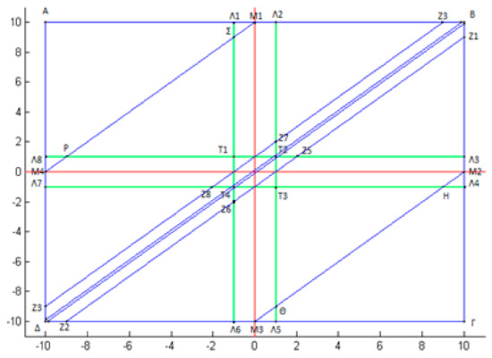
Figure 1. Geometric representation of all pairs of finite precision error mantissae $\left(x,y\right)$. Since these pairs do not belong to the cross ${\Lambda }_1{\Lambda }_2{{\rm T}}_2{\Lambda }_3{\Lambda }_4{{\rm T}}_3{\Lambda }_5{\Lambda }_6{{\rm T}}_4{\Lambda }_7{\Lambda }_8{{\rm T}}_1{\Lambda }_1$, the corresponding joint probability function is restricted within $J=\left(A{\Lambda }_1{{\rm T}}_1{\Lambda }_{8}A\right)\cup \left({\rm B}{\Lambda }_3{{\rm T}}_2{\Lambda }_{2}B\right)\cup \left(\Gamma {\Lambda }_5{{\rm T}}_3{\Lambda }_4\Gamma \right)\cup \left(\Delta {\Lambda }_7{{\rm T}}_4{\Lambda }_6\Delta \right)$.

We point out that the joint probability $f_{XY}\left(x,y\right)$ is a conditional pdf, where $\left(x,y\right)\in J$, in the sense that it satisfies relation ${{\displaystyle \iint }}_J{f}_{XY}\left(x,y\right)dxdy=1$. If the initial pdf $f_{XY}^I\left(x,y\right)$ is defined in a superset of $J$, then, we restrict it to $J$ by means of the conditional probability rule. Notice that the points of the “cross” $C={\Lambda }_1{\Lambda }_2{{\rm T}}_2{\Lambda }_3{\Lambda }_4{{\rm T}}_3{\Lambda }_5{\Lambda }_6{{\rm T}}_4{\Lambda }_7{\Lambda }_8{{\rm T}}_1{\Lambda }_1$ do not belong to $J$, since $x$ and $y$ are mantissae. We again distinguish the sub-cases introduced in Section 3.1.

Case 1.i: $\left|man\left({\alpha }_n\right)man\left({\beta }_n\right)\right|<10$, namely relation (3.4).

Case 1.i.a: $100\le \left|{\alpha }_{n}x+{\beta }_{n}y\right|<UB$, which is (3.6).

In order to determine the sub-domain of $J$, where inequality (3.6) holds, we assume, first, that both ${\alpha }_n,{\beta }_n$ are positive mantissae and we draw the straight lines:

$$E_{100}:{\alpha }_{n}x+{\beta }_{n}y=100,E_{ub}:{\alpha }_{n}x+{\beta }_{n}y=UB.$$

Let $P_a^i$ be the set of points $\left(x,y\right)$ of $J$ that lie between $E_{100}$ and $E_{ub}$, where superscript $i$ and subscript $a$ express the last two letters of the Case in hand. Further, consider the straight lines:

$$E_{-100}:{\alpha }_{n}x+{\beta }_{n}y=-100,E_{-ub}:{\alpha }_{n}x+{\beta }_{n}y=-UB.$$

Let $N_a^i$ be the set of points $\left(x,y\right)$ of $J$ lying between $E_{-100}$ and $E_{-ub}$ and $D_a^i=P_a^i\cup N_a^i$; $D_a^i$ includes all points of $J$ satisfying (3.6). Then, probability $P^{EQ}\left\{\left(x,y\right)\in D_a^i\right\}={{\displaystyle \iint }}_{D_a^i}{f}_{XY}\left(x,y\right)dxdy$. However, in this case only, according to the analysis of Section 3.1, ${\gamma }_n={\alpha }_n{\beta }_n$ is computed with $\xi =2$ additional e. d. d. than $\lambda$. Hence,

$$P^{EQ}\left(2;{\alpha }_n,{\beta }_n\right)=\underset{D_a^i}{{\displaystyle \iint }}{f}_{XY}\left(x,y\right)dxdy.$$

(3.36)

Case 1.i.b: $10\le \left|{\alpha }_{n}x+{\beta }_{n}y\right|<100$, namely inequality (3.8).

For an arbitrary pair of multiplication operands $\left({\alpha }_n,{\beta }_n\right)$, consider, now, the straight lines:

$$E_{10}:{\alpha }_{n}x+{\beta }_{n}y=10\mathrm{and}{E}_{-10}:{\alpha }_{n}x+{\beta }_{n}y=-10.$$

Let $P_b^i$ be the set of points $\left(x,y\right)\in J$ lying between $E_{100}$ and $E_{10}$ and $N_b^i$ be the set of points $\left(x,y\right)\in J$ lying between $E_{-100}$ and $E_{-10}$. $D_b^i=P_b^i\cup N_b^i$ is the entire ensemble of points in $J$ satisfying (3.8), depicted in magenta in Figure 2. Then, probability

$$P^{EQ}\left\{\left(x,y\right)\in D_b^i\right\}\equiv P^{EQ}\left(1;{\alpha }_n,{\beta }_n\right)=\underset{D_b^i}{{\displaystyle \iint }}{f}_{XY}\left(x,y\right)dxdy.$$

(3.37)

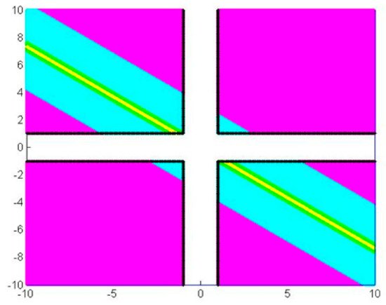
Figure 2. Depiction of the various sub-domains of $J$, which give rise to different numbers of erroneous decimal digits of ${\gamma }_5={\alpha }_5{\beta }_5$, where $\left|man\left({\alpha }_5\right)man\left({\beta }_5\right)\right|<10$. In this example, we have selected ${\alpha }_5=2.3912$ and ${\beta }_5=3.2578$; consequently: (a) the sub-region generating one additional e. d. d. is depicted in magenta, (b) the sub-domain that does not increase the f. p. error is shown in cyan (c) the sub-region relaxing the e. d. d. number by one is depicted in green and (d) the one relaxing the number of e. d. d. by two is shown in yellow. Sub-domains that represent an even greater relaxation of the f. p. e. are too small to appear.

Case 1.i.c: $1\le \left|{\alpha }_{n}x+{\beta }_{n}y\right|<10$, that is (3.10).

Next, in accordance with the previous analysis, we draw the straight lines:

$$E_1:{\alpha }_{n}x+{\beta }_{n}y=1\mathrm{and}{E}_{-1}:{\alpha }_{n}x+{\beta }_{n}y=-1.$$

Then, $P_c^i$ is the sub-domain of $J$ bounded by $E_1$ and $E_{10}$, while $N_c^i$ is the sub-region bounded by $E_{-1}$ and $E_{-10}$. Setting $D_c^i=P_c^i\cup N_c^i$ (cyan area in Figure 2), the probability that a pair $\left(x,y\right)$ of error mantissae satisfies (3.10) is:

$$P^{EQ}\left\{\left(x,y\right)\in D_c^i\right\}\equiv P^{EQ}\left(0;{\alpha }_n,{\beta }_n\right)={{\displaystyle \iint }}_{D_c^i}{f}_{XY}\left(x,y\right)dxdy.$$

(3.38)

Finally, concerning the remaining Case 1.i.d, it holds that:

Case 1.i.d: ${10}^{-k}\le \left|{\alpha }_{n}x+{\beta }_{n}y\right|<{10}^{1-k},k=1,2,3$, namely the condition (3.14).

With a similar reasoning, we define the lines $$\begin{gathered} E_{0.1}:{\alpha }_{n}x+{\beta }_{n}y={10}^{-1},E_{0.01}:{\alpha }_{n}x+ \\ {\beta }_{n}y={10}^{-2},E_{0.001}:{\alpha }_{n}x+{\beta }_{n}y={10}^{-3},E_{-0.1}:{\alpha }_{n}x+{\beta }_{n}y= \\ -{10}^{-1},E_{-0.01}:{\alpha }_{n}x+{\beta }_{n}y=-{10}^{-2},E_{-0.001}:{\alpha }_{n}x+{\beta }_{n}y=-{10}^{-3} \end{gathered}$$ which in turn give rise to the sub-domains $D_{d1}^i$, $D_{d2}^i$ and $D_{d3}^i$. Sub-domains $D_{d1}^i$ and $D_{d2}^i$ are depicted in green and yellow respectively in Figure 2. Eventually, the corresponding probabilities are

$$\begin{array}{c}{P}^{EQ}\left\{\left(x,y\right)\in D_{d1}^i\right\}\equiv P^{EQ}\left(-1;{\alpha }_n,{\beta }_n\right)={{\displaystyle \iint }}_{D_{d1}^i}{f}_{XY}\left(x,y\right)dxdy\\ P^{EQ}\left\{\left(x,y\right)\in D_{d2}^i\right\}\equiv P^{EQ}\left(-2;{\alpha }_n,{\beta }_n\right)={{\displaystyle \iint }}_{D_{d2}^i}{f}_{XY}\left(x,y\right)dxdy\\ P^{EQ}\left\{\left(x,y\right)\in D_{d3}^i\right\}\equiv P^{EQ}\left(-3;{\alpha }_n,{\beta }_n\right)={{\displaystyle \iint }}_{D_{d3}^i}{f}_{XY}\left(x,y\right)dxdy.\end{array}$$

(3.39)

Case 1.ii: $\left|man\left({\alpha }_n\right)man\left({\beta }_n\right)\right|\ge 10$, specifically inequality (3.16).

This case may be treated as Case 1.i; however, here, as stated in Section 3.1, the computing machine performs a right shift in order to restore the product ${\gamma }_n={\alpha }_n{\beta }_n$ in its canonical form. Therefore, product ${\gamma }_n$ is computed with a number of e.d.d. reduced by one with respect to the previous Case 1.i. Thus, briefly, we note the following:

Case 1.ii.a: $100\le \left|{\alpha }_{n}x+{\beta }_{n}y\right|<200$, which is (3.17).

Once again, lines $E_{100}$ and $E_{ub}$, confine $P_a^{ii}\subset J$, and lines $E_{-100}$ and $E_{-ub}$, confine $N_a^{ii}\subset J$. Let, again, ${\mathcal{D}}_a^{ii}=P_a^{ii}\cup N_a^{ii}$ (shown in magenta in Figure 3, for a specific pair of multiplication operands $\left({\alpha }_n,{\beta }_n\right)$). When $\left(x,y\right)\in {\mathcal{D}}_a^{ii}$, product ${\gamma }_n$ is computed with exactly one additional e. d. d. with probability

$$P^{EQ}\left\{\left(x,y\right)\in {\mathcal{D}}_a^{ii}\right\}\equiv P^{EQ}\left(1;{\alpha }_n,{\beta }_n\right)={{\displaystyle \iint }}_{{\mathcal{D}}_a^{ii}}{f}_{XY}\left(x,y\right)dxdy.$$

(3.40)

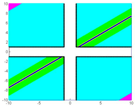
Figure 3. Depiction of the various sub-domains of $J$, which give rise to different numbers of erroneous decimal digits of ${\gamma }_5={\alpha }_5{\beta }_5$, where $\left|man\left({\alpha }_5\right)man\left({\beta }_5\right)\right|\ge 10$. In this example, we have selected ${\alpha }_5=4.6812$ and ${\beta }_5=-6.3178$: therefore (a) the sub-domain generating one additional e. d. d. is depicted in magenta, (b) the sub-region that does not increase the f. p. error is shown in cyan, (c) the sub-domain relaxing the e. d. d. number by one is depicted in green, (d) the one relaxing the number of e. d. d. by two is shown in yellow, while (e) the one relaxing the number of e. d. d. by three is depicted in blue. The sub-domains that represent an even greater relaxation of the f. p. e. are too small to appear.

Case 1.ii.b: $10\le \left|{\alpha }_{n}x+{\beta }_{n}y\right|<100$, i.e., (3.20).

We draw the straight lines $E_{100},E_{10}$ to obtain $P_b^{ii}$, lines $E_{-100},E_{-10}$ to confine $N_b^{ii}$ and we let ${\mathcal{D}}_b^{ii}=P_b^{ii}\cup N_b^{ii}$ (shown in cyan in Figure 3). The probability is

$$P^{EQ}\left(0;{\alpha }_n,{\beta }_n\right)\equiv P^{EQ}\left\{\left(x,y\right)\in {\mathcal{D}}_b^{ii}\right\}={{\displaystyle \iint }}_{{\mathcal{D}}_b^{ii}}{f}_{XY}\left(x,y\right)dxdy.$$

(3.41)

Case 1.ii.c: $1\le \left|{\alpha }_{n}x+{\beta }_{n}y\right|<10$, that is condition (3.22).

We select points $\left(x,y\right)\in J$ lying between $E_{10}$ and $E_1$, forming $P_c^{ii}$ and points $\left(x,y\right)\in J$ lying between $E_{-10}$ and $E_{-1}$, forming $N_c^{ii}$; again, we let ${\mathcal{D}}_c^{ii}=P_c^{ii}\cup N_c^{ii}$ (green area in Figure 3). Now, the probability that f. p. e. is relaxed by one digit is

$$P^{EQ}\left\{\left(x,y\right)\in {\mathcal{D}}_c^{ii}\right\}\equiv P^{EQ}\left(-1;{\alpha }_n,{\beta }_n\right)={{\displaystyle \iint }}_{{\mathcal{D}}_c^{ii}}{f}_{XY}\left(x,y\right)dxdy.$$

(3.42)

Case 1.ii.d: ${10}^{-k}\le \left|{\alpha }_{n}x+{\beta }_{n}y\right|<{10}^{-\left(k-1\right)},k=1,2$, namely the condition (3.24).

Along very similar lines we define sub-domains of $J$, ${\mathcal{D}}_{d1}^{ii}$ and ${\mathcal{D}}_{d2}^{ii}$ (shown in yellow and blue respectively in Figure 3 for a specific pair of operands $\left({\alpha }_n,{\beta }_n\right)$ and $n=5$). We eventually evaluate

$$\begin{array}{c}{P}^{EQ}\left\{\left(x,y\right)\in {\mathcal{D}}_{d1}^{ii}\right\}\equiv P^{EQ}\left(-2;{\alpha }_n,{\beta }_n\right)={{\displaystyle \iint }}_{{\mathcal{D}}_{d1}^{ii}}{f}_{XY}\left(x,y\right)dxdy\\ P^{EQ}\left\{\left(x,y\right)\in {\mathcal{D}}_{d2}^{ii}\right\}\equiv P^{EQ}\left(-3;\alpha ,\beta \right)={{\displaystyle \iint }}_{{\mathcal{D}}_{d2}^{ii}}{f}_{XY}\left(x,y\right)dxdy.\end{array}$$

(3.43)

Case 2: ${\lambda }_a\ne {\lambda }_{\beta }$.

Suppose that without any loss of generality ${\lambda }_a<{\lambda }_{\beta }$ $\left(\iff {\lambda }_a^c>{\lambda }_{\beta }^c\right)$ and that ${\lambda }_{\gamma }$ is the number of erroneous d. d. with which product ${\gamma }_n={\alpha }_n{\beta }_n$; let, moreover, $\xi ={\lambda }_{\gamma }-{\lambda }_{\beta }$.

Notation 3.

In this case, the f. p. error also depends on$\delta$(see Section 3.1). Hence, for the corresponding probability, we use the notation$P^{UN}\left(\xi ,\delta ;{\alpha }_n,{\beta }_n\right)$, where as always, without any loss of generality, we assume that${\alpha }_n$and${\beta }_n$are mantissae and that${\lambda }_a<{\lambda }_{\beta }$. If the opposite inequality${\lambda }_{\alpha }>{\lambda }_{\beta }$holds, then we use the notation$P^{UN}\left(\xi ,\delta ;{\beta }_n,{\alpha }_n\right)$.

We once more consider straight lines $E_{100}^{\delta },E_{-100}^{\delta },E_{10}^{\delta },E_{-10}^{\delta },E_1^{\delta },E_{-1}^{\delta },E_{0.1}^{\delta },E_{-0.1}^{\delta },E_{0.01}^{\delta },E_{-0.01}^{\delta },E_{0.001}^{\delta },E_{-0.001}^{\delta }$, which confine the corresponding sub-domains of $J$: ${\mathcal{G}}_a^i,{\mathcal{G}}_b^i,{\mathcal{G}}_c^i,{\mathcal{G}}_{d1}^i,{\mathcal{G}}_{d2}^i,{\mathcal{G}}_{d3}^i,{\mathcal{G}}_a^{ii},{\mathcal{G}}_b^{ii},{\mathcal{G}}_c^{ii},{\mathcal{G}}_{d1}^{ii},{\mathcal{G}}_{d2}^{ii}$. The probabilities that a pair of mantissae $\left(x,y\right)$ lies in one of the aforementioned domains are:

Case 2.i: $\left|man\left({\alpha }_n\right)man\left({\beta }_n\right)\right|<10$, namely condition (3.4).

Case 2.i.a: $100\le \left|{\alpha }_{n}x+{\beta }_{n}y{10}^{-\delta }\right|$, i.e., (3.28).

$$P^{UN}\left\{\left(x,y\right)\in G_{\alpha }^i\right\}={{\displaystyle \iint }}_{G_{\alpha }^i}{f}_{XY}\left(x,y\right)dxdy=P^{UN}\left(2,\delta ;a_n,{\beta }_n\right)$$

(3.44)

Case 2.i.b: $10\le \left|{\alpha }_{n}x+{\beta }_{n}y·{10}^{-\delta }\right|<100$, that corresponds to (3.29)

$$P^{UN}\left\{\left(x,y\right)\in G_b^i\right\}={{\displaystyle \iint }}_{G_b^i}{f}_{XY}\left(x,y\right)dxdy=P^{UN}\left(1,\delta ;a_n,{\beta }_n\right).$$

(3.45)

Case 2.i.c: $1\le \left|{\alpha }_{n}x+{\beta }_{n}y·{10}^{-\delta }\right|<10$, which is the one of (3.30)

$$P^{UN}\left\{\left(x,y\right)\in G_c^i\right\}\equiv {{\displaystyle \iint }}_{G_c^i}{f}_{XY}\left(x,y\right)dxdy=P^{UN}\left(0,\delta ;{\alpha }_n,{\beta }_n\right).$$

(3.46)

Case 2.i.d:${10}^{-k}\le \left|{\alpha }_{n}x+{\beta }_{n}y·{10}^{-\delta }\right|<{10}^{-\left(k-1\right)},k=1,2,3$, i.e. (3.31)

$$\begin{array}{c}{P}^{UN}\left\{\left(x,y\right)\in G_{d1}^i\right\}\equiv P^{UN}\left(-1,\delta ;{\alpha }_n,{\beta }_n\right)={{\displaystyle \iint }}_{G_{d1}^i}{f}_{XY}\left(x,y\right)dxdy\\ P^{UN}\left\{\left(x,y\right)\in G_{d2}^i\right\}\equiv P^{UN}\left(-2,\delta ;{\alpha }_n,{\beta }_n\right)={{\displaystyle \iint }}_{G_{d2}^i}{f}_{XY}\left(x,y\right)dxdy\\ P^{UN}\left\{\left(x,y\right)\in G_{d3}^i\right\}\equiv P^{UN}\left(-3,\delta ;{\alpha }_n,{\beta }_n\right)={{\displaystyle \iint }}_{G_{d3}^i}{f}_{XY}\left(x,y\right)dxdy.\end{array}$$

(3.47)

Case 2.ii:$\left|man\left({\alpha }_n\right)man\left({\beta }_n\right)\right|\ge 10\left(3.16\right).$

Case 2.ii.a: $100\le \left|{\alpha }_{n}x+{\beta }_{n}y·{10}^{-\delta }\right|<200$, i.e., the inequality of (3.32).

$$P^{UN}\left\{\left(x,y\right)\in {\mathcal{G}}_a^{ii}\right\}\equiv P^{UN}\left(1,\delta ;{\alpha }_n,{\beta }_n\right)={{\displaystyle \iint }}_{{\mathcal{G}}_a^{ii}}{f}_{XY}\left(x,y\right)dxdy.$$

(3.48)

Case 2.ii.b:$10\le \left|{\alpha }_{n}x+{\beta }_{n}y·{10}^{-\delta }\right|<100$, that corresponds to (3.33)

$$P^{UN}\left\{\left(x,y\right)\in {\mathcal{G}}_b^{ii}\right\}\equiv P^{UN}\left(0,\delta ;{\alpha }_n,{\beta }_n\right)={{\displaystyle \iint }}_{{\mathcal{G}}_b^{ii}}{f}_{XY}\left(x,y\right)dxdy.$$

(3.49)

Case 2.ii.c:$1\le \left|{\alpha }_{n}x+{\beta }_{n}y·{10}^{-\delta }\right|<10$, namely inequality (3.34)

$$P^{UN}\left\{\left(x,y\right)\in {\mathcal{G}}_c^{ii}\right\}\equiv P^{UN}\left(-1,\delta ;{\alpha }_n,{\beta }_n\right)={{\displaystyle \iint }}_{{\mathcal{G}}_c^{ii}}{f}_{XY}\left(x,y\right)dxdy.$$

(3.50)

Case 2.ii.d:${10}^{-k}\le \left|{\alpha }_{n}x+{\beta }_{n}y·{10}^{-\delta }\right|<{10}^{-\left(k-1\right)},k=1,2,3$, i.e. the case of (3.35)

$$\begin{array}{c}{P}^{UN}\left\{\left(x,y\right)\in {\mathcal{G}}_{d1}^{ii}\right\}\equiv P^{UN}\left(-2,\delta ;{\alpha }_n,{\beta }_n\right)={{\displaystyle \iint }}_{{\mathcal{G}}_{d1}^{ii}}{f}_{XY}\left(x,y\right)dxdy\\ P^{UN}\left\{\left(x,y\right)\in {\mathcal{G}}_{d2}^{ii}\right\}\equiv P^{UN}\left(-3,\delta ;{\alpha }_n,{\beta }_n\right)={{\displaystyle \iint }}_{{\mathcal{G}}_{d2}^{ii}}{f}_{XY}\left(x,y\right)dxdy.\end{array}$$

(3.51)

3.3. Experimental Confirmation of the Previous Theoretical Results

In order to test the validity of the analysis and the results of previous Section 3.1 and Section 3.2, we have performed the following experiment:

First, we have chosen a set ${\Sigma }^{16}$ consisting of 100,000 couples of randomly chosen mantissae $\left({\alpha }_{16}^i,{\beta }_{16}^i\right)$, having $n=16$ d. d. in the mantissa. We assume that these numbers are all correct, concerning the first 16 d. d.

We have “contaminated” all $\left({\alpha }_{16}^i,{\beta }_{16}^i\right)$, each one with a different error obtained from a normal population, with various values $\sigma$ of the std. In fact, for each $\sigma$, we have produced 25,000 normally distributed error values $\left({\theta }_{\alpha ,i}^N,{\theta }_{\beta ,i}^N\right)$ that will play the role of f. p. e. of ${\alpha }_{16}^i$ and ${\beta }_{16}^i$, should all operations had been made with $n=16$ d. d. precision and the set of contaminated pairs $\left({\tilde{\alpha }}_{16}^i,{\tilde{\beta }}_{16}^i\right)=\left({\alpha }_{16}^i+{\theta }_{\alpha ,i}^N,{\beta }_{16}^i+{\theta }_{\beta ,i}^N\right)$. In addition, we have extended ${\tilde{\alpha }}_{16}^i$ and ${\tilde{\beta }}_{16}^i$ into a representation of $n=64$ d. d., by simply zeroing all decimal digits from the seventeenth one up to 64-th digit.

We have performed all multiplications ${\tilde{\gamma }}_{16}^i={\tilde{\alpha }}_{16}^i·{\tilde{\beta }}_{16}^i$, evidently in 16 d. d. precision, as well as multiplications ${\tilde{\gamma }}_{64}^i={\tilde{\alpha }}_{64}^i·{\tilde{\beta }}_{64}^i$, in 64 d. d. precision. Then, using Definition 2 and Theorem 5, we have obtained the number of e. d. d. of quantity ${\tilde{\gamma }}_{16}^i$, with respect to the e. d. d. of ${\tilde{\alpha }}_{16}^i$ and ${\tilde{\beta }}_{16}^i$ and the set of f. p. e. differences $\#edd\left({\tilde{\gamma }}_i^{16}\right)-max\left\{\#edd\left({\tilde{\alpha }}_{16}^i\right),\#edd\left({\tilde{\beta }}_{16}^i\right)\right\}$. Using this set, we have compared the corresponding experimental frequencies with the theoretical probabilities predicted in the present section, for various standard deviations of f. p. e. Representative results are shown in Table 3, Table 4, Table 5 and Table 6; Table 4 refers to the case where $\#edd\left({\tilde{\alpha }}_{16}^i\right)=\#edd\left({\tilde{\beta }}_{16}^i\right)$, for four arbitrarily chosen pairs $\left({\alpha }_i,{\beta }_i\right)$, shown in Table 3. On the contrary, Table 5 and Table 6 refer to the case where $\#edd\left({\tilde{\beta }}_{16}^i\right)-\#edd\left({\tilde{\alpha }}_{16}^i\right)<0$. Table 5 corresponds to the case in which $\delta =1$, while Table 6 corresponds to the one in which $\delta =2$. From both tables, the excellent agreement between theory and experiment is pretty evident.

Table 3. Four arbitrarily chosen pairs of $\left({\alpha }_{16}^i,{\beta }_{16}^i\right)$.

${\mathit{\alpha }}_{\mathbf{16}}^{\mathit{i}}$	${\mathit{\beta }}_{\mathbf{16}}^{\mathit{i}}$
${\alpha }_1=$ 1.505791937075619	${\beta }_1=$ 5.526986816293506
${\alpha }_2=$ 2.675404049994100	${\beta }_2=$ 2.778498218867048
${\alpha }_3=$ 7.946881519204984	${\beta }_3=$4.557506835434298
${\alpha }_4=$ 5.557116785741900	${\beta }_4=$ 5.549129305868777

Table 4. The theoretical probabilities $P^{EQ}\left(\xi ;{\tilde{\alpha }}_{16}^i,{\tilde{\beta }}_{16}^i\right)$ numerically evaluated, as compared to the actually observed corresponding experimental frequencies of $\xi =\#edd\left({\tilde{\gamma }}_{16}^{\mathsf{\iota }}\right)-\#edd\left({\tilde{\alpha }}_{16}^{\mathsf{\iota }}\right)$.

${\mathit{P}}^{\mathit{E}\mathit{Q}}\left(\mathit{\xi }\mathbf{;}{\tilde{\mathit{\alpha }}}_{\mathbf{16}}^{\mathit{i}}\mathbf{,}{\tilde{\mathit{\beta }}}_{\mathbf{16}}^{\mathit{i}}\right)$Verification. Normally Distributed Contamination σ = 2.2
$\left({\tilde{\mathit{\alpha }}}_{\mathbf{16}}^{\mathit{i}}\mathbf{,}{\tilde{\mathit{\beta }}}_{\mathbf{16}}^{\mathit{i}}\right)$		$\left({\tilde{\mathit{\alpha }}}_{\mathbf{16}}^{\mathbf{1}}\mathbf{,}{\tilde{\mathit{\beta }}}_{\mathbf{16}}^{\mathbf{1}}\right)$	$\left({\tilde{\mathit{\alpha }}}_{\mathbf{16}}^2\mathbf{,}{\tilde{\mathit{\beta }}}_{\mathbf{16}}^{\mathbf{2}}\right)$	$\left({\tilde{\mathit{\alpha }}}_{\mathbf{16}}^{\mathbf{3}}\mathbf{,}{\tilde{\mathit{\beta }}}_{\mathbf{16}}^{\mathbf{3}}\right)$	$\left({\tilde{\mathit{\alpha }}}_{\mathbf{16}}^{\mathbf{4}}\mathbf{,}{\tilde{\mathit{\beta }}}_{\mathbf{16}}^{\mathbf{4}}\right)$
Generation of 2 Additional e. d. d.	Theoretical Probability	0	0	0	0
	Experimental Frequency	0	0	0	0
Generation of 1 Additional e. d. d.	Theoretical Probability	0.648	0.373	${10}^{-5}$	$3.74·{10}^{-9}$
	Experimental Frequency	0.647	0.389	${10}^{-5}$	0
Generation of No Additional e. d. d.	Theoretical Probability	0.338	0.517	0.702	0.622
	Experimental Frequency	0.339	0.503	0.704	0.623
Relaxation of Product’s e. d. d. by 1	Theoretical Probability	0.012	0.099	0.264	0.325
	Experimental Frequency	0.012	0.096	0.262	0.321
Relaxation of Product’s e. d. d. by 2	Theoretical Probability	0.001	0.009	0.031	0.046
	Experimental Frequency	0.001	0.010	0.030	0.049

Table 5. The theoretical probabilities $P^{UN}\left(\xi ,1;{\tilde{\alpha }}_{16}^i,{\tilde{\beta }}_{16}^i\right)$, namely for the case where $\#edd\left({\tilde{\beta }}_{16}^i\right)-\#edd\left({\tilde{\alpha }}_{16}^i\right)=1$, numerically evaluated, as compared to the actually observed corresponding experimental frequencies of $\xi =\#edd\left({\tilde{\gamma }}_{16}^{\mathsf{\iota }}\right)-\#edd\left({\tilde{\beta }}_{16}^{\mathsf{\iota }}\right)$.

${\mathit{P}}^{\mathit{U}\mathit{N}}\left(\mathit{\xi }\mathbf{;}\mathbf{1}\mathbf{;}{\tilde{\mathit{\alpha }}}_{\mathbf{16}}^{\mathit{i}}\mathbf{,}{\tilde{\mathit{\beta }}}_{\mathbf{16}}^{\mathit{i}}\right)$Verification. Normally Distributed Contamination σ = 2.2
$\left({\tilde{\mathit{\alpha }}}_{\mathbf{16}}^{\mathit{i}}\mathbf{,}{\tilde{\mathit{\beta }}}_{\mathbf{16}}^{\mathit{i}}\right)$		$\left({\tilde{\mathit{\alpha }}}_{\mathbf{16}}^{\mathbf{1}},{\tilde{\mathit{\beta }}}_{\mathbf{16}}^{\mathbf{1}}\right)$	$\left({\tilde{\mathit{\alpha }}}_{\mathbf{16}}^{\mathbf{2}}\mathbf{,}{\tilde{\mathit{\beta }}}_{\mathbf{16}}^{\mathbf{2}}\right)$	$\left({\tilde{\mathit{\alpha }}}_{\mathbf{16}}^{\mathbf{3}}\mathbf{,}{\tilde{\mathit{\beta }}}_{\mathbf{16}}^{\mathbf{3}}\right)$	$\left({\tilde{\mathit{\alpha }}}_{\mathbf{16}}^{\mathbf{4}},{\tilde{\mathit{\beta }}}_{\mathbf{16}}^{\mathbf{4}}\right)$
Generation of 2 Additional e. d. d.	Theoretical Probability	0	0	0	0
	Experimental Frequency	0	0	0	0
Generation of 1 Additional e. d. d.	Theoretical Probability	0.008	0.127	0	0
	Experimental Frequency	0.008	0.147	0	0
Generation of No Additional e. d. d.	Theoretical Probability	0.870	0.873	0.867	0.631
	Experimental Frequency	0.872	0.853	0.870	0.633
Relaxation of Product’s e. d. d. by 1	Theoretical Probability	0.112	$2·{10}^{-4}$	0.133	0.369
	Experimental Frequency	0.110	$1·{10}^{-4}$	0.130	0.367
Relaxation of Product’s e. d. d. by 2	Theoretical Probability	0.009	0	0	$4.23·{10}^{-6}$
	Experimental Frequency	0.009	0	0	0

Table 6. The theoretical probabilities $P^{UN}\left(\xi ,2;{\tilde{\alpha }}_{16}^i,{\tilde{\beta }}_{16}^i\right)$, namely for the case where $\#edd\left({\tilde{\beta }}_{16}^i\right)-\#edd\left({\tilde{\alpha }}_{16}^i\right)=2$, numerically evaluated, as compared to the actually observed corresponding experimental frequencies of $\xi =\#edd\left({\tilde{\gamma }}_{16}^{\mathsf{\iota }}\right)-\#edd\left({\tilde{\beta }}_{16}^{\mathsf{\iota }}\right)$.

${\mathit{P}}^{\mathit{U}\mathit{N}}\left(\mathit{\xi }\mathbf{,}\mathbf{2}\mathbf{;}{\tilde{\mathit{\alpha }}}_{\mathbf{16}}^{\mathit{i}},{\tilde{\mathit{\beta }}}_{\mathbf{16}}^{\mathit{i}}\right)\mathbf{Verification}\mathbf{.}\mathbf{Normally}\mathbf{Distributed}\mathbf{Contamination}\mathsf{\sigma }\mathbf{=}\mathbf{2.2}$
$\left({\tilde{\mathit{\alpha }}}_{\mathbf{16}}^{\mathit{i}}\mathbf{,}{\tilde{\mathit{\beta }}}_{\mathbf{16}}^{\mathit{i}}\right)$		$\left({\tilde{\mathit{\alpha }}}_{\mathbf{16}}^{\mathbf{1}}\mathbf{,}{\tilde{\mathit{\beta }}}_{\mathbf{16}}^{\mathbf{1}}\right)$	$\left({\tilde{\mathit{\alpha }}}_{\mathbf{16}}^{\mathbf{2}}\mathbf{,}{\tilde{\mathit{\beta }}}_{\mathbf{16}}^{\mathbf{2}}\right)$	$\left({\tilde{\mathit{\alpha }}}_{\mathbf{16}}^{\mathbf{3}}\mathbf{,}{\tilde{\mathit{\beta }}}_{\mathbf{16}}^{\mathbf{3}}\right)$	$\left({\tilde{\mathit{\alpha }}}_{\mathbf{16}}^{\mathbf{4}}\mathbf{,}{\tilde{\mathit{\beta }}}_{\mathbf{16}}^{\mathbf{4}}\right)$
Generation of 2 Additional e. d. d.	Theoretical Probability	0	0	0	0
	Experimental Frequency	0	0	0	0
Generation of 1 Additional e. d. d.	Theoretical Probability	0.004	0.123	0	0
	Experimental Frequency	0.003	0.134	0	0
Generation of No Additional e. d. d.	Theoretical Probability	0.996	0.877	0.865	0.626
	Experimental Frequency	0.997	0.866	0.872	0.637
Relaxation of Product’s e. d. d. by 1	Theoretical Probability	0	0	0.135	0.374
	Experimental Frequency	0	0	0.128	0.363
Relaxation of Product’s e. d. d. by 2	Theoretical Probability	0	0	0	0
	Experimental Frequency	0	0	0	0

We have repeated the previous step, using uniformly distributed “contamination numbers” ${\theta }_i^U$, in the interval [${10}^{-16},{10}^{-3}]$, producing numbers ${\widehat{\alpha }}_{16}^i={\alpha }_{16}^i+{\theta }_i^U$.

By repeating all actions of previous Step 3 for the case of uniform contamination, the obtained results have confirmed an excellent agreement between theory and practice.

A set of concrete experiments and associated tables.

We have randomly chosen $25,000$ couples of mantissae terms $\left({\alpha }_{16}^i,{\beta }_{16}^i\right)$, covering all cases referred to in Section 3.1 and Section 3.2. We have embedded both ${\alpha }_{16}^i$ and ${\beta }_{16}^i$ in $64$ d. d. precision, as described previously in the present sub-section, thus forming corresponding couples $\left({\alpha }_{64}^i,{\beta }_{64}^i\right)$. We have contaminated each such pair $\left({\alpha }_{16}^i,{\beta }_{16}^i\right)$ with 25,000 normally distributed error values for various distinct values of standard deviation $\sigma$. In this way, we have generated $25,000$ corresponding contaminated pairs $\left({\tilde{\alpha }}_{16}^i,{\tilde{\beta }}_{16}^i\right)$.

We have performed all $25,000$ multiplications ${\tilde{\gamma }}_{16}^i={\tilde{\alpha }}_{16}^i·{\tilde{\beta }}_{16}^i$, as well as the associated products ${\gamma }_{64}^i={\alpha }_{64}^i·{\beta }_{64}^i$ and, finally, we have evaluated the number of erroneous decimal digits of ${\tilde{\gamma }}_{16}^i$ by comparing it with ${\gamma }_{64}^i$.

The results of this experiment for a specific value of $\sigma$ are shown in Table 3, Table 4, Table 5 and Table 6. In Table 3, four arbitrarily chosen different pairs $\left({\alpha }_{16}^i,{\beta }_{16}^i\right),i=1,2,3,4$ are presented. Table 4 refers to the case where $\#edd\left({\tilde{\alpha }}_{16}^i\right)=\#edd({\tilde{\beta }}_{16}^i$), for the corresponding contaminated pairs $\left({\tilde{\alpha }}_{16}^i,{\tilde{\beta }}_{16}^i\right)$, while Table 5 and Table 6 refer to the cases in which $\delta =1$ and $\delta =2$ respectively, where $\delta =\#edd\left({\tilde{\beta }}_{16}^i\right)-\#edd\left({\tilde{\alpha }}_{16}^i\right)$.

For all arbitrarily chosen contaminated pairs $\left({\tilde{\alpha }}_{16}^i,{\tilde{\beta }}_{16}^i\right)$, we have evaluated the theoretical probabilities introduced in Section 3.1, numerically. From all tables, the excellent agreement between theory and experiment is pretty evident. We would like to point out that this excellent agreement appears in all performed experiments, concerning $10-ths$ of different values of standard deviation $\sigma$.

4. Analysis of the Case of Many Successive Multiplications

In this section, we will compute the probability that $M$ successive multiplications generate $\lambda$ erroneous d. d. in the final product.

In fact, suppose that any two numbers, ${\gamma }_n^0$ and ${\beta }_n^0$, are multiplied in a computing machine using $n$ decimal digits (d. d.) in the mantissa; let ${\gamma }_n^1={\gamma }_n^0{\beta }_n^0$. Next, ${\gamma }_n^1$ is multiplied by an arbitrary number, say ${\beta }_n^1$, giving rise to ${\gamma }_n^2={\gamma }_n^1{\beta }_n^1$ and so on. The analysis of Section 3 indicates that a different number of erroneous d. d. emerges as it is analytically presented in Table 1 and Table 2. Therefore, in order to estimate the number of erroneous decimal digits (e. d. d.) accumulated in a result of many successive multiplications, one may employ the following:

• The mantissa $y$ of the finite precision error (f. p. e.) accumulated at an arbitrary quantity, say $\alpha$, is a random variable, already symbolized as $Y$. Therefore, when two quantities ${\alpha }_n$ and ${\beta }_n$ are multiplied with f. p. e. mantissae $x$ and $y$, then the f. p. error of the product ${\gamma }_n=a_n{\beta }_n$ is itself a random variable.
• As before, without any loss of generality, suppose that ${\lambda }_{\beta }$ is the maximum number of e. d. d. between ${\alpha }_n$ and ${\beta }_n$. Then, reminding that the symbol “$\#$” stands for cardinal number, $\#edd\left({\gamma }_n\right)$ differ from ${\lambda }_{\beta }$ by $\xi$ e. d. d. Evidently, $\xi$ is a random variable itself, having integer values $=2,1,0,-1,-2,\dots$.
• In Section 3, we have given a method for evaluating the probabilities $P^{EQ}\left(\xi ;{\alpha }_n,{\beta }_n\right)$, namely the probability that product ${\gamma }_n$ is computed with a number of erroneous decimal digits (e. d. d.) differing by ξ decimal digits from the common e. d. d. of ${\alpha }_n and {\beta }_n$. In the same section, we have also proposed a method for evaluating the probabilities $P^{UN}\left(\xi ,\delta ;{\alpha }_n,{\beta }_n\right)$, i.e., the probability that product ${\gamma }_n$ is computed with a number of e. d. d. differing by ξ decimal digits from the maximum number of e. d. d. between ${\alpha }_n and {\beta }_n$. For brevity, in the present section, we will assume that in all successive multiplications the worst case always takes place, namely that the two multiplication operands share the same number of correct decimal digits (c. d. d.). Moreover, we will momentarily simplify notation by letting $P_2=P^{EQ}\left(2;{\alpha }_n,{\beta }_n\right)$, $P_1=P^{EQ}\left(1;{\alpha }_n,{\beta }_n\right)$, $P_{-k}=P^{EQ}\left(-k;{\alpha }_n,{\beta }_n\right), k=0,1,2,\dots$.
• We have performed an extensive number of multiplications ${\gamma }_n^{i+1}={\gamma }_n^i{\beta }_n^i, i=0,1,2,\dots$, where, initially, ${\gamma }_n^0$ and ${\beta }_n^0$ are chosen uniformly from the interval $\left(-10, 10\right)$ and with $n$ d. d. precision in the mantissa. Then, the f. p. e. mantissa $x$ of the product ${\gamma }_n^{i+1}$ follows a normal distribution with zero (0) mean value and standard deviation $\sigma \in \left[1.1, 6.5\right]$. Hence, probabilities $P_j, j=2,1,0,-1,-2,\dots$ are immediately obtained via the analysis of Section 3. However, the present analysis is valid for any distribution of error mantissae that gives rise to a set of probabilities $P_j$.
• For brevity and simplicity reasons, we shall assume that the ensemble of probabilities $P_j$ remains unaltered throughout the entire successive multiplications process. Should any concern on that arise, as we will explicitly state below, a proper source code may be used in order to compute $P^{EQ}\left(\xi ;{\alpha }_n,{\beta }_n\right)$ dynamically, while the essence of the following analysis remains intact.

Subsequently, we will compute the probability that $M$ successive multiplications generate $\lambda$ erroneous d. d. in the final product ${\gamma }_n^M$. In fact, suppose that one performs $M$ successive multiplications and that $i_1$ of them produce two additional e. d. d. ($\xi =2$), $i_2$ of them produce one additional e. d. d. ($\xi =1$), $i_3$ of them produce no additional e. d. d. ($\xi =0$) and $i_k$ products “enjoyed” relaxation of the number of e. d. d. by $k$ digits ($\xi =-k$). Then, the number $\omega$ of e. d. d. with which the final product of $M$ successive multiplications is obtained, is given by $\omega ={\displaystyle \sum }_{\mu }{\xi }_{\mu }{i}_{\mu }$. We are interested in the mean value and variation of quantity $\omega$. To achieve that, we shall present a set of quite general lemmas and theorems; for this reason, for the present section only, we shall introduce an alternative, equivalent notation described below:

Notation 4.

Let$\xi$be defined as in the previous analysis above. Then, one may define events$A_1, A_2, A_3, \dots$ as follows:$A_1:\xi =2$,$A_2:\xi =1$,$A_3:\xi =0$,$A_{3+\kappa }:\xi =-\kappa , \kappa =1,2,\dots$, where events$A_{3+\kappa }$refer to error correction by$\kappa$digits.

Intimately associated with Notation 4 is the following:

Hypothesis 1.

In order to obtain proper bounds of the number $\lambda$ of e. d. d. accumulated in the final product of $M$ successive multiplications, it is sufficient to assume that at each one of these $M$ successive multiplications, the corresponding probabilities $P^{EQ}\left(\xi ;{\gamma }_n,{\beta }_n\right)$ remain constant.

Under this assumption, we let:

$$P_1=P^{EQ}\left(2;{\gamma }_n,{\beta }_n\right)=P\left(A_1\right),P_2=P^{EQ}\left(1;{\gamma }_n,{\beta }_n\right)=P\left(A_2\right),P_{3+k}=P^{EQ}\left(-\kappa ;{\gamma }_n,{\beta }_n\right)=P\left(A_{3+k}\right), k=0,1,2,\dots .$$

In order to obtain the aforementioned bounds for $\lambda$, we shall employ the subsequent quite general results.

Lemma 1.

Consider a multinomial distribution with possible outcomes $A_1, A_2, \dots ,A_N$, with corresponding probability of appearance $P_1, P_2, \dots ,P_N$. Suppose that one performs an experiment $M$ times, whose outcome is modeled by this distribution. Let the first event with outcome $A_1$ be observed $i_1$ times, the second event with outcome $A_2$ $i_2$ times and so on. Then, quantity $\omega =A_1{i}_1+\dots +A_{{\rm N}}{i}_{{\rm N}}={\displaystyle \sum }_{\mu =1}^{{\rm N}}{A}_{\mu }{i}_{\mu }$ has a mean value $\overline{\omega }$ and a variance $S_{\omega }^2$:

$$\overline{\omega }=M{{\displaystyle \sum }}_{\mu =1}^{{\rm N}}{A}_{\mu }{P}_{\mu }.$$

(4.1)

$$S_{\omega }^2={\rm M}\left({{\displaystyle \sum }}_{\mu =1}^{{\rm N}}{A}_{\mu }^2{P}_{\mu }-{{\displaystyle \sum }}_{\mu =1}^{{\rm N}}{A}_{\mu }^2{P}_{\mu }^2-2{{\displaystyle \sum }}_{i=1}^{{\rm N}}{{\displaystyle \sum }}_{j=i+1}^{{\rm N}}{A}_i{A}_j{P}_i{P}_j\right).$$

(4.2)

Proof of Lemma 1.

The probability that ω occurs is given by

$$P\left(\omega \right)=\left(\begin{array}{c}M\\ i_1\end{array}\right)P_1^{i_1}\left(\begin{array}{c}M-i_1\\ i_2\end{array}\right)P_2^{i_2}\dots P_{N-1}^{i_{N-1}}{P}_{{\rm N}}^{M-\left(i_1+i_2+\dots +i_{N-1}\right)}.$$

(4.3)

For the mean value $\overline{\omega }$: By definition:

$$\begin{gathered} \overline{\omega }={\displaystyle \sum }_{i_1}{\displaystyle \sum }_{i_2}\dots {\displaystyle \sum }_{i_N}\left[A_1{i}_1+A_2{i}_2+\dots +A_{{\rm N}}{i}_{{\rm N}}\right]P\left(\omega \right)\begin{array}{c}\left(4.3\right)\\ \iff \end{array} \\ \overline{\omega }={\displaystyle \sum }_{i_1}{\displaystyle \sum }_{i_2}\dots {\displaystyle \sum }_{i_N}{A}_1{i}_1\left(\begin{array}{c}M\\ i_1\end{array}\right)P_1^{i_1}\left(\begin{array}{c}M-i_1\\ i_2\end{array}\right)P_2^{i_2}\left(\begin{array}{c}M-i_1-i_2\\ i_3\end{array}\right)P_3^{i_3}\dots \left(\begin{array}{c}M-i_1-\dots -i_{N-2}\\ i_{N-1}\end{array}\right)P_{N-1}^{i_{N-1}}{P}_{{\rm N}}^{M-\left(i_1+i_2+\dots +i_{N-1}\right)}+\dots \\ +{\displaystyle \sum }_{i_1}{\displaystyle \sum }_{i_2}\dots {\displaystyle \sum }_{i_N}{A}_N{i}_N\left(\begin{array}{c}M\\ i_1\end{array}\right)P_1^{i_1}\left(\begin{array}{c}M-i_1\\ i_2\end{array}\right)P_2^{i_2}\left(\begin{array}{c}M-i_1-i_2\\ i_3\end{array}\right)P_3^{i_3}\dots \left(\begin{array}{c}M-i_1-\dots -i_{N-2}\\ i_{N-1}\end{array}\right)P_{N-1}^{i_{N-1}}{P}_N^{M-\left(i_1+i_2+\dots +i_{N-1}\right)} \end{gathered}$$

We treat each multiple sum separately. Therefore,

$$\begin{gathered} \overline{{\omega }_1}={\displaystyle \sum }_{i_1}{\displaystyle \sum }_{i_2}\dots {\displaystyle \sum }_{i_{N-1}}{A}_1{i}_1\left(\begin{array}{c}M\\ i_1\end{array}\right)P_1^{i_1}\left(\begin{array}{c}M-i_1\\ i_2\end{array}\right)P_2^{i_2}\dots P_{N-1}^{i_{N-1}}{P}_N^{M-\left(i_1+i_2+\dots +i_{N-1}\right)} \\ ={{\displaystyle \sum }}_{i_1=0}^M{A}_1{i}_1\left(\begin{array}{c}M\\ i_1\end{array}\right)P_1^{i_1}\dots {{\displaystyle \sum }}_{i_{N-1}=0}^{M-i_1-\dots -i_{N-2}}\left(\begin{array}{c}M-i_1-\dots -i_{N-2}\\ i_{N-1}\end{array}\right)P_{N-1}^{i_{N-1}}{P}_N^{M-i_1-\dots -i_{N-1}} \\ =A_1{P}_{1}M{{\displaystyle \sum }}_{i_1=1}^{M-1}\frac{\left(M-1\right)!}{\left(i_1-1\right)!\left(M-i_1\right)!}{P}_1^{i_1-1}\dots {{\displaystyle \sum }}_{i_{N-1}=0}^{M-i_1-\dots -i_{N-2}}\frac{\left(M-i_1-\dots -i_{N-2}\right)!}{i_{N-1}!\left(M-i_1-\dots -i_{N-1}\right)!}{P}_{N-1}^{i_{N-1}}{P}_N^{M-i_1-\dots -i_{N-1}} \end{gathered}$$

$i_{N-1}$-sum is a version of the identity

$${\left(P_1+P_2+\dots +P_{{\rm N}}\right)}^M={{\displaystyle \sum }}_{i_1=0}^M\left(\begin{array}{c}M\\ i_1\end{array}\right)P_1{}^{i_1}{\left(P_2+\dots +P_{{\rm N}}\right)}^{M-i_1.}$$

Hence,

$${\overline{\omega }}_1=A_1{P}_{1}M.$$

(4.4)

By employing the same approach, we obtain the previous relation (4.1)

$$\overline{\omega }={\overline{\omega }}_1+{\overline{\omega }}_2+\dots +{\overline{\omega }}_N\Rightarrow \overline{\omega }=M{{\displaystyle \sum }}_{\mu =1}^{{\rm N}}{A}_{\mu }{P}_{\mu }.$$

For the variance $S_{\omega }^2$: By definition:

$$S_{\omega }^2={\displaystyle \sum }_{\omega }{\omega }^{2}P\left(\omega \right)-{\overline{\omega }}^2.$$

(4.5)

By employing the previously given expression for $\omega$, we obtain:

$$\begin{gathered} S_{\omega }^2={{\displaystyle \sum }}_{i_1=0}^M\dots {{\displaystyle \sum }}_{i_{N-1}=0}^{M-i_1-\dots -i_{N-2}}{\left[A_1{i}_1+\dots +A_N{i}_N\right]}^2\cdot \left(\begin{array}{c}M\\ i_1\end{array}\right)P_1^{i_1}\dots \left(\begin{array}{c}M-i_1-\dots -i_{N-2}\\ i_{N-1}\end{array}\right)P_{N-1}^{i_{N-1}}{P}_{{\rm N}}^{M-\left(i_1+i_2+\dots +i_{N-1}\right)}- \\ {M}^2{\left({{\displaystyle \sum }}_{\mu =1}^{{\rm N}}{A}_{\mu }{P}_{\mu }\right)}^2. \end{gathered}$$

Expanding ${\left[A_1{i}_1+\dots +A_N{i}_N\right]}^2$, we obtain the partial sums:

$$\begin{gathered} s_1^2={\displaystyle \sum }_{i_1=0}^M\dots {\displaystyle \sum }_{i_{N-1}=0}^{M-i_1-\dots -i_{N-2}}{A}_1{}^2{i}_1{}^2\left(\begin{array}{c}M\\ i_1\end{array}\right)P_1^{i_1}\left(\begin{array}{c}M-i_1\\ i_2\end{array}\right)P_2^{i_2}\dots \left(\begin{array}{c}M-i_1-\dots -i_{N-2}\\ i_{N-1}\end{array}\right)P_{N-1}^{i_{N-1}}{P}_{{\rm N}}^{M-\left(i_1+i_2+\dots +i_{N-1}\right)} \\ =A_1{}^2{\displaystyle \sum }_{i_1=0}^M{i}_1{}^2\left(\begin{array}{c}M\\ i_1\end{array}\right)P_1^{i_1}\dots {\displaystyle \sum }_{i_{N-1}=0}^{M-i_1-\dots -i_{N-2}}\left(\begin{array}{c}M-i_1-\dots -i_{N-1}\\ i_N\end{array}\right)P_{N-1}^{i_{N-1}}{P}_N^{M-\left(i_1+i_2+\dots +i_{N-1}\right)}\iff \\ {s}_1^2={\displaystyle \sum }_{i_1=0}^M\dots {\displaystyle \sum }_{i_{N-1}=0}^{M-i_1-\dots -i_{N-2}}{A}_1{}^2{i}_1{}^2\left(\begin{array}{c}M\\ i_1\end{array}\right)P_1^{i_1}\left(\begin{array}{c}M-i_1\\ i_2\end{array}\right)P_2^{i_2}\dots \left(\begin{array}{c}M-i_1-\dots -i_{N-1}\\ i_N\end{array}\right)P_{N-1}^{i_{N-1}}{P}_{{\rm N}}^{M-\left(i_1+i_2+\dots +i_{N-1}\right)} \\ =A_1{}^2{{\displaystyle \sum }}_{i_1=0}^M{i}_1\left(i_1-1\right)\left(\begin{array}{c}M\\ i_1\end{array}\right)P_1^{i_1}{\left(P_2+\dots +P_N\right)}^{M-i_1}+A_1{}^2{{\displaystyle \sum }}_{i_1=0}^M{i}_1\left(\begin{array}{c}M\\ i_1\end{array}\right)P_1^{i_1}{\left(P_2+\dots +P_N\right)}^{M-i_1} \\ =A_1{}^{2}M\left(M-1\right)P_1^2{\displaystyle \sum }_{i_1=2}^{M-2}\frac{\left(M-2\right)!}{\left(i_1-2\right)!\left(M-i_1\right)!}{P}_1^{i_1-2}{\left(P_2+\dots +P_N\right)}^{M-i_1} \\ +A_1{}^2{P}_{1}M{\displaystyle \sum }_{i_1=1}^{M-1}\frac{\left(M-1\right)!}{\left(i_1-1\right)!\left(M-i_1\right)!}{P}_1^{i_1-1}{\left(P_2+\dots +P_N\right)}^{M-i_1} \end{gathered}$$

$$s_1^2=A_1{}^{2}M\left(M-1\right)P_1^2+A_1{}^2{P}_{1}M$$

Following an analogous process for the other similar terms of quantity $S_{\omega }^2$, we obtain

$$s_{\mu }^2=A_{\mu }{}^{2}M\left(M-1\right)P_{\mu }^2+A_{\mu }{}^2{P}_{\mu }M,\mu =1,2,\dots ,N$$

We now calculate the cross-product

$$\begin{gathered} s_{1,2}^2={{\displaystyle \sum }}_{i_1=0}^M\dots {{\displaystyle \sum }}_{i_{N-1}=0}^{M-i_1-\dots -i_{N-2}}2A_1{A}_2{i}_1{i}_2\left(\begin{array}{c}M\\ i_1\end{array}\right)P_1^{i_1}\left(\begin{array}{c}M-i_1\\ i_2\end{array}\right)P_2^{i_2}\dots \left(\begin{array}{c}M-i_1-\dots -i_{N-2}\\ i_{N-1}\end{array}\right)P_{N-1}^{i_{N-1}}{P}_{{\rm N}}^{M-i_1-\dots -i_{N-1}}\iff \\ {s}_{1,2}^2=2A_1{A}_2{P}_1{P}_{2}M\left(M-1\right){{\displaystyle \sum }}_{i_1=1}^{M-2}\left(\begin{array}{c}M-2\\ i_1-1\end{array}\right)P_1^{i_1-1}{{\displaystyle \sum }}_{i_2=1}^{M-i_1}\left(\begin{array}{c}M-i_1\\ i_2-1\end{array}\right)P_2^{i_2-1}{\left(P_3+\dots +P_N\right)}^{M-i_1-i_2}\iff \\ {s}_{1,2}^2=2A_1{A}_2{P}_2{P}_{1}M\left(M-1\right). \end{gathered}$$

Similarly, for the remaining cross-products, we obtain

$$s_{i,j}^2=2A_i{A}_j{P}_i{P}_{j}M\left(M-1\right),i,j=1,2,\dots ,N,i\ne j.$$

Summing up $s_{\mu }^2$ and $s_{i,j}^2$, we eventually obtain

$$S_{\omega }^2={\displaystyle \sum }_{\mu =1}^{{\rm N}}{s}_{\mu }^2+{\displaystyle \sum }_{\begin{array}{c}i,j=1\\ i<j\end{array}}^{{\rm N}}{s}_{i,j}^2-{\overline{\omega }}^2$$

$$\iff S_{\omega }^2={\rm M}\left[{\displaystyle \sum }_{\mu =1}^{{\rm N}}{A}_{\mu }^2{P}_{\mu }-{\displaystyle \sum }_{\mu =1}^{{\rm N}}{A}_{\mu }^2{P}_{\mu }^2-2{\displaystyle \sum }_{i=1}^{{\rm N}}{\displaystyle \sum }_{j=i+1}^{{\rm N}}{A}_i{A}_j{P}_i{P}_j\right].$$

□

This Lemma along with the central limit theorem, offer the following:

Lemma 2.

Suppose that one executes $M\ge 30$ successive multiplications. Then, the number of erroneous d. d. generated in the product obtained after these multiplications, $\omega ={{\displaystyle \sum }}_{\mu =1}^{{\rm N}}{A}_{\mu }{i}_{\mu }$, follows a normal distribution with mean value $\overline{\omega }$ and variance $S_{\omega }^2$ given by (4.1) and (4.2).

We will apply all the previous results to the three more important cases, described below.

Case 1. The worst case, where in all multiplications $\left|man\left({\gamma }_n^i\right)man\left({\beta }_n^i\right)\right|<10$ holds.

Case 2. The most favorable case, where $\left|man\left({\gamma }_n^i\right)man\left({\beta }_n^i\right)\right|\ge 10$ always holds.

Case 3. The general case, where the distribution of $\left|man\left({\gamma }_n^i\right)man\left({\beta }_n^i\right)\right|$ is arbitrary.

Case 1. If at each multiplication, inequality (3.4) holds, namely

$$\left|man\left({\alpha }_n\right)man\left({\beta }_n\right)\right|<10,$$

then we choose the following values around which the corresponding probabilities are more frequently encountered:

• $\xi =2$: $P^{EQ}\left(2;{\gamma }_n^i,{\beta }_n^i\right)=P_1\approx O\left({10}^{-9}\right)$ (i.e., almost negligible). We repeat that we use probabilities $P^{EQ}$ only, since we consider the worst case as far as f. p. error generation and accumulation is concerned, namely that $\#edd\left({\gamma }_n^i\right)=\#edd\left({\beta }_n^i\right)$.
• $\xi =1$: $P^{EQ}\left(1;{\gamma }_n^i,{\beta }_n^i\right)=P_2\approx 0.5530$.
• $\xi =0$: $P^{EQ}\left(0;{\gamma }_n^i,{\beta }_n^i\right)=P_3\approx 0.3934$.
• $\xi =-1$: $P^{EQ}\left(-1;{\gamma }_n^i,{\beta }_n^i\right)=P_4\approx 0.0457$.
• $\xi =-2$: $P^{EQ}\left(-2;{\gamma }_n^i,{\beta }_n^i\right)=P_5\approx 7.8·{10}^{-3}$.
• $\xi =$−3: $P^{EQ}\left(-3;{\gamma }_n^i,{\beta }_n^i\right)=P_6\approx O\left({10}^{-6}\right)$. (i.e., almost negligible).

Therefore, if $M$ such successive multiplications take place, then, the overall number $\omega ={{\displaystyle \sum }}_{\mu =1}^{{\rm N}}{A}_{\mu }{i}_{\mu }$ of generated e. d. d. follows a multinomial distribution, which may be very well approximated by a normal distribution with $\overline{\omega }=0.4917\cdot M$ and $S_{\omega }^2=0.3881\cdot M$, $M\ge 30$. Hence, quantity $z=\frac{\omega -\overline{\omega }}{S_{\omega }}$ follows a standard Gauss distribution, i.e., $z ~ N\left(0,1\right)$.

However, now, inequality $\left|man\left({\alpha }_n\right)man\left({\beta }_n\right)\right|<10$ (3.4) holds, thus, $\overline{\omega }$ is positive and inequality $\frac{\omega -\overline{\omega }}{S_{\omega }}\ge -4.2649$ holds with confidence 99.999%; coefficient $-4.2649$ corresponds to the aforementioned confidence level. With this level of significance, the accumulated number $\omega$ of erroneous d. d. in the final product, after $M$ successive multiplications, obeying inequality (3.4), satisfies relation

$$\omega \ge -4.2649S_{\omega }+\overline{\omega }.$$

(4.6)

However, in this case, the right-hand side of inequality (4.6) is always positive and, moreover, is a monotonically increasing function of $M$. Consequently, the accumulated number $\omega$ of erroneous decimal digits of every product ${\gamma }_n^i, i=1, 2, \dots , M$, tends to rapidly increase even for a particularly small number of successive multiplications $M$. This is fully supported by the contents of Table 7 and Table 8, below.

Table 7. $F_g$ is a percentage of multiplications in which inequality (3.16) holds. Thus, when $F_g<50\%$ holds, then ${\gamma }_n^i$ becomes completely erroneous after a relatively small number of multiplications, in full accordance with the theoretical predictions. These predictions are based on the results of Theorems 1, 3 and 5, refer to the lower bound of the expected e. d. d. for each $F_g$ and they are presented in the last column for confidence level $1-{10}^{-5}$. For each $F_g$ the experimental and theoretical results manifest an excellent agreement.

Percentage of Successive Multiplications Satisfying $\left|\mathit{m}\mathit{a}\mathit{n}\left( {\mathit{\alpha }}_{\mathit{n}}^{\mathit{i}}\right)\mathit{m}\mathit{a}\mathit{n}\left({\mathit{\beta }}_{\mathit{n}}^{\mathit{i}}\right)\right|\mathbf{\ge }\mathbf{10}$.	Number of Successive Multiplications after Which Product ${\mathit{\gamma }}_{\mathit{n}}^{\mathit{i}}\mathbf{=}{\mathit{\alpha }}_{\mathit{n}}^{\mathit{i}}\mathbf{·}{\mathit{\beta }}_{\mathit{n}}^{\mathit{i}}$ Was Computed with All 16 d. d. Erroneous.	Theoretical Lower Bounds for $\#\mathit{e}\mathit{d}\mathit{d}\left({\mathit{\gamma }}_{\mathit{n}}^{\mathit{i}}\right)$ Obtained via Theorems 1, 3 and 5.
0.0578	92	15.85
0.0718	89	14.00
0.0841	88	12.92
0.0926	90	12.93
0.1160	104	15.15
0.1360	107	14.40
0.1862	108	10.66
0.2310	131	11.58
0.2734	175	15.22
0.4053	328	12.90
0.4562	459	10.12
0.4591	489	11.46
0.4826	577	6.39

Table 8. Demonstration of the results of experiment associated with Case 3, described in the Section 4: 3 × 10⁵ successive multiplications ${\gamma }_n^i={\alpha }_n^i·{\beta }_n^i$ have been performed for various percentages $F_g$ of them satisfying $\left|man\left({\alpha }_n^i\right)man\left({\beta }_n^i\right)\right|\ge 10$. The obtained maximum and average numbers of e. d. d. are in full accordance with Theorems 1, 3 and 5. In fact, when $F_g>50\%$ holds, then the evaluated products manifest a considerable resistance to finite precision error. The closest to 1 $F_g$ is, the smaller the number of erroneous digits with which all ${\gamma }_n^i$ are computed, exactly as predicted by the theoretical analysis.

Percentage of Successive Multiplications Satisfying $\left|\mathit{m}\mathit{a}\mathit{n}\left({\mathit{\alpha }}_{\mathit{n}}^{\mathit{i}}\right)\mathit{m}\mathit{a}\mathit{n}\left({\mathit{\beta }}_{\mathit{n}}^{\mathit{i}}\right)\right|\mathbf{\ge }\mathbf{10}$	Maximum Number of e. d. d. with Which Product ${\mathit{\gamma }}_{\mathit{n}}^{\mathit{i}}\mathbf{=}{\mathit{\alpha }}_{\mathit{n}}^{\mathit{i}}\mathbf{·}{\mathit{\beta }}_{\mathit{n}}^{\mathit{i}}$ Has Been Computed, $\mathit{i}\mathbf{\le }\mathbf{3}\mathbf{·}{\mathbf{10}}^{\mathbf{5}}$	Average Number of e. d. d. Accumulated in All Products ${\mathit{\gamma }}_{\mathit{n}}^{\mathit{i}}\mathbf{=}{\mathit{\alpha }}_{\mathit{n}}^{\mathit{i}}\mathbf{·}{\mathit{\beta }}_{\mathit{n}}^{\mathit{i}}$ $\mathbf{,}\mathit{i}\mathbf{=}\mathbf{1}\mathbf{,}\mathbf{2}\mathbf{,}\mathbf{\dots }\mathbf{,}\mathbf{3}\mathbf{·}{\mathbf{10}}^{\mathbf{5}}$
0.5014	13	7.7761
0.5029	12	7.2217
0.5051	11	6.9437
0.5063	11	6.8764
0.5076	11	6.6435
0.5131	10	6.1244
0.5143	10	6.0928
0.5154	10	6.0165
0.5171	10	5.9189
0.5204	10	5.7784
0.5260	9	5.5140
0.5300	9	5.4266
0.5404	9	5.1647
0.5481	9	5.0070
0.5588	8	4.8098
0.5899	8	4.4619
0.6182	8	4.1856
0.7742	6	3.4101
0.8422	6	3.0055
0.8702	5	2.9013
0.8913	5	2.8306
0.9195	5	2.7292
0.9412	5	2.6463
0.9519	4	2.6105

Theorem 1.

Let us assume that a number of$M$successive multiplications${\gamma }_n^{i+1}={\gamma }_n^i{\beta }_n^i,i=0, \dots , M-1$is performed and that for every multiplication, inequality$\left|man\left({\gamma }_n^i\right)man\left({\beta }_n^i\right)\right|<10$holds. In this case, the product${\gamma }_n^i, i=1,\dots , M$is prone to serious finite precision error accumulation. We also assume that Hypothesis 1 now holds. Let, in the$N$-th iteration the number$\omega$, $\omega ={{\displaystyle \sum }}_{\mu =1}^{{\rm N}}{A}_{\mu }{i}_{\mu }$, be the number of erroneous d. d. with which quantity${\gamma }_n^N$has been evaluated. Then, it holds that

$$\omega \ge C\left(\alpha \right)·S_{\omega }+\overline{\omega },$$

(4.7)

where$\alpha$is the desired level of significance and$C\left(\alpha \right)$is the lower bound of the corresponding confidence interval.

The theorem holds for any desired level of significance$\alpha$. Due to the fact that quantity$\left(C\left(\alpha \right)·S_{\omega }+\overline{\omega }\right)$is always positive in this case and it is a monotonically increasing function of$M$, quantity$\omega =\#edd\left({\gamma }_n^N\right)$tends to increase rapidly, even for particularly small numbers of$M$.

Hypothesis 2 and Associated Notation 5.

Suppose that probabilities $P_i=P^{EQ}\left(\xi ;{\gamma }_n^i,{\beta }_n^i\right)$ do not remain constant throughout the successive multiplications, but on the contrary, they depend on the current $i-th$ multiplication. In this case, we consider the following events and the corresponding probabilities for an arbitrary multiplication, say the $i-th$ one:

$A_{1,i}=\left\{2 e.d.d. added to {\gamma }_n^i\right\}$; $P_{1,i}=P^{EQ}\left(2;{\gamma }_n^i,{\beta }_n^i\right),$

$A_{2,i}=\left\{1 e.d.d. added to {\gamma }_n^i\right\}$; $P_{2,i}=P^{EQ}\left(1;{\gamma }_n^i,{\beta }_n^i\right),$,

$A_{3,i}=\left\{no e.d.d. added to {\gamma }_n^i\right\}$; $P_{3,i}=P^{EQ}\left(0;{\gamma }_n^i,{\beta }_n^i\right),$

$A_{4,i}=\left\{reduction of {\gamma }_n^i e.d.d. by one\right\}$; $P_{4,i}=P^{EQ}\left(-1;{\gamma }_n^i,{\beta }_n^i\right)$etc.

If one adopts the above Hypothesis 2, the following result holds:

Theorem 2.

Under the conditions imposed by Hypothesis 2, one may dynamically compute the exact (up to $\pm 1$ d. d.) number of erroneous decimal digits, which are accumulated at the $i-th$, arbitrary, product ${\gamma }_n^i$, $i=1,2,\dots ,M$ by applying the method introduced in Section 3. This dynamic computation of $\#edd\left({\gamma }_n^i\right)$ can be made by a rather straightforward code based on the results of Section 3.

Case 2. Now, we assume that at each one of the $M$ successive multiplications, inequality (3.16) holds, i.e., that

$$\left|man\left({\gamma }_n\right)man\left({\beta }_n\right)\right|\ge 10.$$

Then, consider the following associated, quite representative probabilities, in accordance with the analysis of Section 3.2, Case 1.ii:

• Probability that $A_1 \left(\xi =2\right)$ occurs is $P_1=0$, since in this case equality $\xi =2$ can never occur.
• Probability that $A_2\left(\xi =1\right)$ occurs is $P_2=6.146·{10}^{-4}$.
• Probability that $A_3 \left(\xi =0\right)$ occurs is $P_3=0.7468$.
• Probability that $A_4 \left(\xi =-1\right)$ occurs is $P_4=0.2224$.
• Probability that $A_5 \left(\xi =-2\right)$ occurs is $P_5=0.02720$.
• Probability that $A_6 \left(\xi =-3\right)$ occurs is $P_6=0.002979$.

As a rule, the probabilities of events $A_6, A_7,\dots$ are pretty small, practically zero; however, the entire analysis is absolutely valid if one incorporates the (very small) corresponding probabilities in it. Hence, according to Lemma 1, $\overline{\omega }=-0.2851\cdot M$ and $S_{\omega }^2=0.2783\cdot M$.

We would like to emphasize that in this case, the mean value $\overline{\omega }$ of generated e. d. d. is negative.

Now, quantity $z=\frac{\omega -\overline{\omega }}{S_{\omega }}$ follows a standard Gauss distribution, i.e., $z~N\left(0,1\right)$. Hence, inequality $\frac{\omega -\overline{\omega }}{S_{\omega }}\le 4.2649$ holds with confidence 99.999%. With this confidence level, the accumulated number $\omega$ of e. d. d. after $M$ successive multiplications obeying (3.16), satisfies

$$\omega \le 4.2649S_{\omega }+\overline{\omega }.$$

(4.8)

Here, $4.2649S_{\omega }+\overline{\omega }$ is a monotonically decreasing function of $M$. Thus, the accumulated number $\omega$ of e. d. d. remains very close to zero, even for a very large number of multiplications. This has been fully experimentally verified as described in Section 4. Hence, the following holds:

Theorem 3.

Suppose that a number of $M$ successive multiplications ${\gamma }_n^{i+1}={\gamma }_n^i{\beta }_n^i,i=0, \dots , M-1$ is performed. For every such multiplication, let inequality $\left|man\left({\gamma }_n^i\right)man\left({\beta }_n^i\right)\right|\ge 10$ (3.16) holds. Then, for all practical purposes, these multiplications accumulate a negligible amount of f. p. error on the product ${\gamma }_n^{i+1}={\gamma }_n^i{\beta }_n^i$ for all $i=0, \dots , M.$

Moreover, the number of erroneous decimal digits (e. d. d.) accumulated in the arbitrary ${\gamma }_n^i$ product, is, as a rule, a decreasing function of $i$.

If, in addition, Hypothesis 1 is adopted, then the number$\omega$of e. d. d. accumulated in the$i$-th multiplication satisfies inequality (4.8).

The theorem holds for any desired level of significance$\alpha$, the only difference being the coefficient of$S_{\omega }$.

By a complete analogy with Theorem 2, one may adopt Hypothesis 2, in which case the following result holds:

Theorem 4.

Under the conditions imposed by Hypothesis 2, one may dynamically compute the exact (up to $\pm 1$ d. d.) number of erroneous decimal digits, which are accumulated at the $i-th$, arbitrary, product ${\gamma }_n^i$, $i=1,2,\dots ,M$ by applying the method introduced in Section 3. This dynamic computation of $\#edd\left({\gamma }_n^i\right)$ can be made by a rather straightforward code based on the results of Section 3.

Case 3. In the general case, either inequality $\left|man\left({\gamma }_n^i\right)man\left({\beta }_n^i\right)\right|\ge 10$ (3.16) or inequality $\left|man\left({\gamma }_n^i\right)man\left({\beta }_n^i\right)\right|<10$ (3.4) arbitrarily holds. Then, in order to obtain a rigorous estimation of the number of e. d. d. in each multiplication, together with the corresponding probability, one must know the statistical distribution of $\left|man\left({\gamma }_n^i\right)man\left({\beta }_n^i\right)\right|$, as compared to ten (10). In general, these distributions may highly depend on the algorithm in hand. However, in order to obtain an estimation of the corresponding generated f. p. error, we will state the very interesting example where both $\left|man\left({\gamma }_n^i\right)\right|$ and $\left|man\left({\beta }_n^i\right)\right|$ follow a uniform distribution in the interval $\left[1,\right.\left.10\right)$. In fact, in this case, the set of $\left({\gamma }_n^i,{\beta }_n^i\right)$ in the ${\gamma }_n^i{\beta }_n^i$-plain satisfying (3.4), is the 2D domain bounded by the straight lines ${\gamma }_n^i=1$ and ${\beta }_n^i=1$ and the hyperbola ${\gamma }_n^i{\beta }_n^i=10$. Dually, the 2D domain for which the alternative inequality (3.16) holds, is the one limited by the straight lines ${\gamma }_n^i=10$, ${\beta }_n^i=10$ and the same hyperbola. Then, we follow the results of Section 3 and we use the graphical representation associated with the square of Figure 1 for the probability density function $f_{XY}^{UN}\left(x,y\right)=\frac{1}{81}$, defined on this square except the cross. Consequently, in a rather straightforward manner, we obtain $P\left\{\left|man\left({\gamma }_n^i\right)man\left({\beta }_n^i\right)\right|<10\right\}=\frac{1}{81}{{\displaystyle \int }}_1^{10}\frac{10}{{\beta }_n^i}d{\beta }_n^i=\frac{1}{81}{\left[10\ln \left({\beta }_n^i\right)\right]}_1^{10}\cong 0.7157$.

In case that there is no discernible distribution of $\left|man\left({\gamma }_n^i\right)man\left({\beta }_n^i\right)\right|$ within the course of the algorithm, we may dynamically calculate the finite precision error accumulation for every product in order to estimate the accumulation of the finite precision error in the algorithm in general, as described in Theorems 2 and 4; we remind that Theorem 2 refers to the worst case in which $\left|man\left({\gamma }_n^i\right)man\left({\beta }_n^i\right)\right|<10$ always holds, while Theorem 4 is connected to the dual inequality (3.16), which is most favorable from the point of view of generation of finite precision error during multiplication. In any case, the following holds:

Theorem 5.

Suppose again that during $M$ successive multiplications ${\gamma }_n^{i+1}={\gamma }_n^i{\beta }_n^i,i=0, \dots , M-1$ and that for a fraction, say $F_g$, of these multiplications, inequality (3.16) holds, while for the other fraction $F_s=1-F_g$ of them inequality (3.4) holds. Then, concerning the f. p. error accumulation in the products ${\gamma }_n^i, i=1, \dots , M$, the following two cases hold:

(i) 

if $F_g>0.5$, product ${\gamma }_n^i$ tends to behave as described in Case 2, i.e., the overall number of e. d. d. of ${\gamma }_n^i, i=1, \dots , M$ is restrained. The closer to 1 fraction $F_g$ is, the greater the restriction of the number of e. d. d. accumulated in products ${\gamma }_n^i$ (see Table 8).

(ii) 

If $F_g<0.5$, the accumulated f. p. error in the products ${\gamma }_n^i$ is amplified. The closer to 0 $F_g$ is, the more rapidly the f. p. e. accumulated in products ${\gamma }_n^i$ grows (Table 7).

The theoretical approach and the associated results introduced in the present Section 4, have been fully confirmed experimentally, as it will be described in Section 6 of the present work.

5. Comparing the Finite Precision Error Generation and Accumulation during Execution of the Same Algorithm Including Successive Multiplications, with Different Finite Word Length/Precision

We shall begin by giving a brief description of the goal of the present section: consider an algorithm $\mathcal{A}$, involving multiplications at each iteration. We execute $\mathcal{A}$ first with $n$ decimal digits in the mantissa (say $n\ge 7$) and simultaneously with $m$ decimal digits (d. d.) in the mantissa, where we assume that $m\ge 2n+7$, using exactly the same input in both cases. Consider any quantity $\gamma$ of $\mathcal{A}$ and let ${\gamma }_n^i$ be the value of this quantity at the $i-\mathrm{th}$ iteration of $\mathcal{A}$, where all calculations are made with precision of $n$ d. d. in the mantissa. Similarly, let ${\gamma }_m^i$ be the value of this quantity at the same iteration of $\mathcal{A}$, when all operations are made with precision of $m$ d. d. In the present section, we will compare the number of erroneous d. d. with which any such two quantities ${\gamma }_n^i,{\gamma }_m^i$ are calculated and, in particular, for the difference $\Delta =\left|\#edd\left({\gamma }_n^i\right)-\#edd\left({\gamma }_m^i\right)\right|$.

In Section 4 we have concluded that, independently of the finite word length, the number of e. d. d. of any product $\gamma$ follows a normal distribution if the number of successive multiplications which generated $\gamma$, is greater than or equal to 30. Thus, the difference in the number of e. d. d. between ${\gamma }_n^i$ and ${\gamma }_m^i$ also follows a normal distribution with mean value zero and a variance that can be immediately estimated from the results of Section 4. Hence, one may deduce:

Theorem 6.

Suppose that an algorithm $\mathcal{A}$ including an arbitrary number of successive multiplications, is executed in parallel with two different finite word lengths corresponding to $n$ and $m$ decimal digits (d. d.). Let the two representations of an arbitrary quantity $\gamma$ of $\mathcal{A}$ be ${\gamma }_n$ and ${\gamma }_m$ respectively, in these two finite word lengths. Consider the random variable

$$\Lambda =\left\{number of e. d. d. accumulated in {\gamma }_m\right\}-\left\{number of e. d. d. accumulated in {\gamma }_n\right\}.$$

(5.1)

$\Lambda$follows a normal distribution with mean value zero and variance$2S_{\omega }^2$, where$S_{\omega }^2$is given in (4.2). Let$F_{m,n}\left(t\right)$be the cumulative distribution function of$\Lambda$’s normal distribution. Then, the probability that$\Delta =\left|\Lambda \right|$is greater than$\zeta$d. d. (where, clearly,$\zeta \ge 0$) is given by

$$P\left(\Delta >\zeta \right)=2\left(1-F_{m,n}\left(\zeta \right)\right).$$

(5.2)

Corollary 1.

Based on the analysis introduced in Section 3 and Section 4, one may deduce in a quite straightforward manner that the probabilities that ${\gamma }_n^i$ and ${\gamma }_m^i$ differ in absolute value by $\Delta \ge 7$ decimal digits, is practically zero. This holds true for arbitrarily large number $M$ of successive multiplications executed in A.

Theorem 7.

As in Theorem 6, we let $\mathcal{A}$ be executed in parallel with the two different finite word lengths $n$ and $m$, where $m>2n+7$. Then, for an arbitrary quantity $\gamma$ of $\mathcal{A}$, the following hold:

1. 

We project ${\gamma }_m$ to $n$ d. d. in the mantissa, obtaining a restricted representation ${\tilde{\gamma }}_n$ of ${\gamma }_m.$ We compare ${\gamma }_n$ and ${\tilde{\gamma }}_n$ by means of Definitions 1 and 2. If the obtained result is $\kappa$ e. d. d. $(\kappa <n)$, then we deduce that precisely the last $\kappa$ digits of ${\gamma }_n$ are erroneous.

2. 

We also deduce that ${\gamma }_m$ has at most $\kappa +7$ e. d. d. or, equivalently, that the first $m–\kappa –7$ d. d. of ${\gamma }_m$ are correct.

3. 

As long as $\kappa <n$ holds, then, ${\tilde{\gamma }}_n$ is a fully correct representation of $\gamma$ with $n$ d. d.

6. Experiments That Fully Support the Theoretical Analysis

In this section, we shall introduce a number of experiments that have been specifically designed by the authors, in order to test the validity and the reliability of the theoretical analysis and results presented in the previous sections.

6.1. Description of a First Class of Experiments That Confirm the Theoretical Approach

Aiming at testing methodology and the associated theoretical results introduced in Section 3 and Section 4, we have proceeded as follows: first, we have selected a set $S_n$ of ${10}^6$ randomly chosen floating point numbers having 16 decimal digits (d. d.) in the mantissa (subscript $n$ stands for 16); the elements of this set come from a uniform distribution. All numbers were expressed in scientific form.

Next, we have extended each number $a_n$ of $S_n$ into a 40 d. d. representation, in scientific form, setting the last 24 d. d. of each number’s mantissa to zero. Thus, we have obtained floating point numbers $a_m$ forming set $S_m$ ($m=40$).

Subsequently, we have chosen an arbitrary, momentarily fixed value of $F_g$ in the interval $\left[0, 1\right]$. We have performed $F_g·{10}^9$ multiplications with $n=16$ d. d., for which the multiplication operands ${\alpha }_n, {\beta }_n$ satisfied (3.16). Next, we have performed $\left(1-F_g\right)·{10}^9$ multiplications with 16 d. d. word length, where the opposite inequality, (3.4), namely that the mantissa of the product terms have absolute value smaller than 10, holds. We have ensured that no repetition of any multiplication occurred.

The very same multiplications have been repeated with 40 d. d. precision, among the corresponding numbers $a_m\in S_m$. Suppose that two numbers ${\alpha }_n$, ${\beta }_n\in S_n$, when multiplied, generate ${\gamma }_n^1$ with finite precision error (f. p. e.) $x_n^1\ge 0$, while ${\gamma }_m^1$ is generated with f. p. e. $x_m^1\ge 0$. These errors have been computed via Definition 2 and Theorems 5 and 6 introduced in Section 5. More specifically:

(i)

We have restricted ${\gamma }_m^1$ into $n=16$ d. d., thus obtaining the number ${\tilde{\gamma }}_n^1$.

(ii)

According to Theorem 6, ${\tilde{\gamma }}_n^1$ is a correct representation of product $\gamma$ having $n=16$ decimal digits in its mantissa.

(iii)

We have compared ${\gamma }_n^1$ and ${\tilde{\gamma }}_n^1$ using Definitions 1 and 2, i.e., by forming their difference $\left|{\gamma }_n^1-{\tilde{\gamma }}_n^1\right|$. In this way, we have obtained the exact number of erroneous decimal digits (e. d. d.) with which quantity ${\gamma }_n^1$ has been evaluated.

By merging the obtained products ${\gamma }_n^1 \mathrm{and} {\gamma }_m^1$ in two distinct ensembles, we have formed two new sets, $S_n^1, S_m^1$, being in a natural biunivocal relation (${\gamma }_n^1, {\gamma }_m^1$).

Moreover, for the same value $F_g$, we have performed $F_g·{10}^9$ multiplications between ${\alpha }_n^1, {\beta }_n^1\in S_n^1$, satisfying (3.16), as well as $\left(1-F_g\right)·{10}^9$ multiplications where (3.4) holds, obtaining ${10}^9$ products ${\gamma }_n^2$. Again, during the aforementioned process, no repetition of any multiplication occurred. The very same multiplications have been performed with 40 decimal digits precision, between corresponding elements of set $S_m^1$, obtaining products ${\gamma }_m^2$. The erroneous d. d. of ${\gamma }_n^1$ have been computed using ${\gamma }_m^1$, as described above based on the results of Section 2 and Section 5. We let products ${\gamma }_n^2$ and ${\gamma }_m^2$ form sets $S_n^2$ and $S_m^2$ respectively, maintaining the natural biunivocal relation (${\gamma }_n^2, {\gamma }_m^2$).

We continued in this way, forming sets ($S_n^3,S_m^3)$,$\dots , \left(S_n^i,S_m^i\right)$, etc. with the same factor $F_g$. In all these cases we evaluated the number of e. d. d. with which products ${\gamma }_n^i$, are computed as it has been previously described in connection with ${\gamma }_n^1$ and ${\gamma }_m^1$. In addition, whenever an exponent exceeded a large absolute value (e.g., 50) during the previous process, it was set to zero, since the exponent ${10}^{\tau }, \tau \in \mathbb{Z},$ of the scientific form plays no role in the f. p. e. generation and accumulation in the multiplication process in general. We have taken this action, in order to avoid possible effects of overflow or underflow in consecutive multiplications, since these easily spotted problems have nothing to do with the present study. However, we have kept the overall exponent of each product by simple recursive additions.

We have repeated the aforementioned experiment for various values of $F_g$, where always $F_g\in \left[0,1\right]$. At this point, we have distinguished two additional sub-cases: (a) $F_g<0.5$ and (b) $F_g>0.5$.

Sub-case (a) is quite analogous to Case 1, for which inequality (3.4) holds permanently. Specifically, the obtained products ${\gamma }_n^i={\alpha }_n^i{\beta }_n^i$, have been calculated with all digits erroneous after a relatively small number of iterations, as shown in Table 7. The smaller fraction $F_g$, the more serious the f. p. error is.

On the contrary, Sub-case (b) is quite similar to Case 2, in the sense that products ${\gamma }_n^i={\alpha }_n^i{\beta }_n^i$ manifested substantially smaller f. p. e. accumulation, as Table 8 manifests. In full accordance with the theoretical analysis, the smaller $F_g$, the smaller the accumulated f. p. e. in ${\gamma }_n^i$ is.

6.2. A Second Class of Experiments for Testing the Theoretical Analysis Concerning Successive Multiplications

Case 1. All Successive Multiplications Satisfy Inequality (3.4), $\left|man\left({\alpha }_n^i\right)man\left({\beta }_n^i\right)\right|<10$ $\left(\iff F_g\cong 0\right)$.

In connection to it, we have performed the following experiment: we have implemented an artificial algorithm, which forces all successive multiplications to satisfy (3.4). The flow chart of this algorithm is the following:

Starting from an arbitrary number ${\beta }_0\in \left[1,\left.10\right)\right.$, we express it with a certain number $n$ of decimal digits (d. d.), as well as with $m=2n+10$ d. d. We then multiply ${\beta }_0$ by itself in both precisions. In case ${\beta }_0^2$ exceeds ten, then we subtract a properly selected positive integer $c_0$, from ${\beta }_0$ in both precisions; we do so, in order that $1\le {\beta }_0^2<10$ now holds. We stress that $c_0$ is adequately selected to be an integer in order that its subtraction from the initial ${\beta }_0$ does not add any e. d. d. to ${\beta }_0$; in all performed experiments, we ensured this by checking the number of e. d. d. of the difference $\left({\beta }_0-c_0\right)$, via Definition 2. By comparing product ${\beta }_0^2$ in both precisions, we calculate the erroneous decimal digits (e. d. d.) of ${\beta }_0^2$ in the $n$ digits precision. Next, we set the exponent of ${\beta }_0^2$ equal to zero, in order to avoid overflow or underflow and we let the obtained mantissa of ${\beta }_0^2$ be a new number, ${\beta }_1$, expressed in both precisions. Then, we repeat the previous actions by letting ${\beta }_1$ play the role of ${\beta }_0$ and we evaluate and store the number of e. d. d. with which ${\beta }_1^2$ is computed, after ensuring that ${\beta }_1^2\in \left[1,\left.10\right)\right.$, via a proper subtraction ${\beta }_1-c_1$, as before. We continue this process until the obtained ${\beta }_i^2$ is calculated in the $n$ digits precision with all its digits erroneous, while we have ensured that ${\beta }_i^2\in \left[1,\left.10\right)\right.$.

We have executed this algorithm for 1000 different initial values of ${\beta }_0$, always belonging to the interval $\left[1,\left.10\right)\right.$. The obtained maximum number of iterations for which ${\beta }_i^2$ was totally erroneous is shown in Table 9 for various values of precision $n$. Thus, we obtain the particularly important result that ${\beta }_i^2$ is totally erroneous after an impressively small number of iterations, in comparison to the employed precision, in full accordance with the theory and in particular with Theorem 1 of Section 4.

Table 9. Table demonstrating the number of iterations after which the output of the algorithm described in Case 1 of the present Section, offered totally erroneous results, for various employed finite word lengths $n$. The results are in full accordance with the theoretical analysis presented in the previous sub-sections. The experimentally observed results are in excellent agreement with the content of Theorem 1 of Section 4.

Employed Precision in Decimal Digits	Number of Iterations after Which All Digits of ${\mathit{\beta }}_{\mathit{i}}^{\mathbf{2}}$ Were Erroneous, Independently of the Choice of ${\mathit{\beta }}_{\mathbf{0}}$
16	61
64	249
128	484
256	967
512	1915
1024	3843
2048	7670
4096	15,285

Case 2. All Successive Multiplications Satisfied $\left|man\left({\alpha }_n^i\right)man\left({\beta }_n^i\right)\right|\ge 10\left(\iff F_g\cong 1\right)$.

We have, again, performed an additional experiment, in which we have written an artificial algorithm, that forces all successive multiplications to satisfy $\left|man\left({\alpha }_n^i\right)man\left({\beta }_n^i\right)\right|\ge 10$. Indeed, this algorithm is quite similar to the one described in connection with Case 1 above and it has the following flow chart:

Starting, again, from an arbitrary number ${\beta }_0\in \left[1,\left.10\right)\right.$, we express it in both $n$ and $m=2n+10$ d. d. precision. We then execute ${\beta }_0\cdot {\beta }_0$ in both precisions. In case ${\beta }_0^2$ is smaller than ten, then we add a properly selected positive integer $c_0$ to ${\beta }_0$ in both precisions, so as ${\beta }_0^2\ge 10$. We stress that ${\beta }_0+c_0$ never manifests any e. d. d. By comparing product ${\beta }_0^2$ in both precisions, we calculate and store the $n$-precision number’s e. d. d., again by means of Definition 2 and Theorem 5. Next, we set the exponent of ${\beta }_0^2$ to zero, once more to avoid overflow or underflow and we let the obtained mantissa of ${\beta }_0^2$ be a new number ${\beta }_1$ expressed in both precisions. Next, we repeat the previous actions by letting ${\beta }_1$ play the role of ${\beta }_0$ and we store and evaluate the number of e. d. d. with which number ${\beta }_1^2$ is computed, after ensuring that ${\beta }_1^2\in \left[1,\left.10\right)\right.$ by adding a proper $c_1$ to ${\beta }_1$, if necessary. We repeated this process for an arbitrarily large number of iterations, while monitoring the f. p. error of ${\beta }_1^2$.

We have executed this algorithm ${10}^{10}$ times in 16 and 42 d. d. precision for 1000 initial values of ${\beta }_0$, always belonging to the interval $\left[1,\left.10\right)\right.$. The experiment has shown that the number of erroneous decimal digits with which ${\beta }_1^2$ has been calculated never exceeded two (2), while the mean value of these e. d. d. remained always pretty close to zero, even for the larger numbers of iterations of the algorithm, in full accordance with Theorem 3.

6.3. Description of a Third Experiment That Fully Supports the Theoretical Results regarding the Case of Successive Multiplications with a Varying Word Length

We have experimentally tested the correctness of Theorem 7 of Section 5, by performing $M$ successive multiplications as described in Section 4. However, now, each multiplication has been executed three times with 16, 40 and 128 d. d. in the mantissa. In this way for each product $\gamma$ we have obtained three representations, ${\gamma }_{16},{\gamma }_{40}$ and ${\gamma }_{128}$ in parallel. Next, we have restricted ${\gamma }_{40}$ to 16 d. d., obtaining representation ${\tilde{\gamma }}_{16}$ as described before. Similarly, we have projected ${\gamma }_{128}$ to both 16 and 40 d. d., obtaining the corresponding representations ${\widehat{\gamma }}_{16}$ and ${\widehat{\gamma }}_{40}$. Eventually, we have compared ${\gamma }_{16}$ with ${\tilde{\gamma }}_{16}$ and ${\widehat{\gamma }}_{16}$ by means of Definitions 1 and 2; we have also compared ${\tilde{\gamma }}_{16}$ with ${\widehat{\gamma }}_{16}$ and ${\gamma }_{40}$ with ${\widehat{\gamma }}_{40}$ via the same method. The obtained results are shown in Table 10 and fully justify the aforementioned Theorems of Section 5, but also of Section 4.

Table 10. Comparison of the number of erroneous decimal digits (e. d. d.) accumulated in all the intermediate results of 10⁸ successive multiplications. All these multiplications have been executed in parallel, with 16, 40 and 128 d. d. in the mantissa. All obtained experimental results fully support the theoretical analysis introduced in Section 5 and in particular the content of Theorems 6 and 7.

Minimum Erroneous Decimal Digits Difference Between 16 and 40 Decimal Digits Representation.	−3
Maximum Erroneous Decimal Digits Difference Between 16 and 40 Decimal Digits Representation	3
Mean Erroneous Decimal Digits Difference Between 16 and 40 Decimal Digits Representation	−0.0945
Maximum Number of Erroneous Decimal Digits in the 16 Decimal Digits Representation	12
Maximum Number of Erroneous Decimal Digits in the 40 Decimal Digits Representation	32

7. Eventual Applications Associated with the Present Work

In the section in hand, we shall present and highlight an ensemble of possible and probable applications, which will be based in the analysis and methodology introduced here. Thus:

• In certain applications, like the ones that will be described below, it is preferable and/or necessary to use finite elements methods, which employ polynomials of high order to approximate the considered function on each element, usually called “higher order basis functions”. In this approach, if the higher order basis functions are of order $n$, then one must use elements consisting of $\left(n+1\right)$ nodes; moreover, one frequently uses the following basis functions ([20]):

  $$\widehat{{\psi }_i}\left(\xi \right)=\frac{\left(\xi -{\xi }_1\right)\dots \left(\xi -{\xi }_j\right)\dots \left(\xi -{\xi }_{i-1}\right)\left(\xi -{\xi }_{i+1}\right)\dots \left(\xi -{\xi }_{n+1}\right)}{\left({\xi }_i-{\xi }_1\right)\dots \left({\xi }_i-{\xi }_j\right)\dots \left({\xi }_i-{\xi }_{i-1}\right)\left({\xi }_i-{\xi }_{i+1}\right)\dots \left({\xi }_i-{\xi }_{n+1}\right)},$$

  (7.1)

  where (a) $i$ is the cardinal number of the node in hand, $i=1,2,\dots ,n+1$, (b) $j$ represents the cardinal number of the other nodes of the specific element, hence $j=1,2,3,\dots ,n+1, j\ne i$, (c) $\xi$ is the independent variable of the polynomial basis function and (d) evidently ${\xi }_j$, $j=1,2,3,\dots ,n+1$ is the value that this variable acquires on the $j-th$ element of the node in hand.

It is rather clear that both the nominator and the denominator in relation (7.1) are results of successive multiplications.

However, even in the case of second order basis functions, one employs the basis functions:

$$\widehat{{\psi }_1}\left(\xi \right)=\frac{1}{2}\xi \left(\xi -1\right),\widehat{{\psi }_2}\left(\xi \right)=1-{\xi }^2,\widehat{{\psi }_3}\left(\xi \right)=\frac{1}{2}\xi \left(\xi +1\right),$$

(7.2)

which includes multiplications. Consequently, the entire previous analysis may be applied immediately, so that together with $\widehat{{\psi }_i}\left(\xi \right), i=1,2,\dots ,n+1$ computation, the user may know the exact number of erroneous decimal digits with which this quantity has been evaluated, each time. Clearly, in case that the numerical value of such a basis function for a certain $\xi$ is highly or even totally “contaminated”, then the user may immediately receive a corresponding signal.

Therefore, more specifically, this method can be applied to the subsequent applications:

• In research associated with the modelling of the fatigue of materials employed in the rail-wheel system ([21,22]).
• In the study of rail corrugation ([23,24]).
• In the study of the influence of bending on the value of friction coefficient ([25]).
• In tackling important classes of contact problems in elatostatics ([26,27]).
• In the investigation and analysis of the spatial stress-strain states of a pipe with respect to its corrosion damage, taking into account various types of complex loading ([28]).
• In real time analysis of local damage in wear-and-fatigue tests, whenever finite elements methods are required/applied ([29]).

It is worthwhile noticing that in many of the aforementioned studies the involved models frequently include multiplications; consequently the approach introduced in the present manuscript may also be proved helpful in associated numerical experiments.

B.

The sequence of powers of a real number.

Consider a single real number, say $\beta >0$. Moreover, consider the sequence of powers of $\beta$, usually computed recursively by means of the following succession of multiplications:

$$\begin{gathered} z_0=\beta ·\beta \\ {z}_1=z_0·z_0 \\ {z}_2=z_1·z_1 \\ \dots \\ {z}_n=z_{n-1}·z_{n-1},n\in \mathbb{N}. \end{gathered}$$

Suppose that the numerical value of $\beta >0$ is such that, statistically, multiplication $z_{n-1}·z_{n-1}$, $n\in \mathbb{N}$, satisfies inequality (3.4)

$$\left|man\left(z_{n-1}\right)·man\left(z_{n-1}\right)\right|<10,$$

more frequently than the opposite one (3.16), namely

$$\left|man\left(z_{n-1}\right)·man\left(z_{n-1}\right)\right|\ge 10$$

Then, according to the previous analysis, one expects that $z_n$ will continually be evaluated with a larger number of erroneous decimal digits (e. d. d.), as $n$ grows. To verify/demonstrate that, we have employed $\beta =1.12$, we have generated sequence $z_n$ of the powers of $\beta$ by means of the aforementioned sequence of successive multiplications and we have evaluated the exact number of e. d. d. with which $z_n$ is calculated each time; the determination of the exact number of erroneous d. d. has been made as described in Section 5 and Section 6, using $n=16$ decimal digits word length and $m=40$ decimal digits precision. The associated results are depicted in Figure 4, from which it is evident that after the impressively small number of 55 iterations, the power $z_n$ is computed with all its digits erroneous.

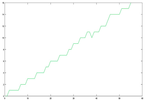
Figure 4. The evolution of the number of the erroneous decimal digits (e. d. d.) accumulated in the power ${\beta }^{2n}, \beta =1.12$, due to finite precision error. The abscissa represents the recursions’ cardinal number, while $y’y$ axis represents the number of e. d. d. Number $\beta$ has been chosen in such a way, so as inequality $\left|man\left(z_{n-1}\right)·man\left(z_{n-1}\right)\right|<10$ holds more frequently than the dual one (3.16). As a consequence, the number of e. d. d. grows rapidly, in full accordance with the analysis and the results of Section 4 and Section 6.

We must emphasize that, in order to circumvent the effects of overflow, each time we have multiplied the mantissae of $z_{n-1}$ only and not the entire number $z_{n-1}$. Equivalently, whenever the exponent of $z_n$ exceeded a rather large number, say $E\left(z_n\right)=50$, then we have divided with ${10}^{E\left(z_n\right)}$. However, we have registered the power’s exponent each time by simple recursive additions. It is important to stress that, in both these approaches the number of erroneous decimal digits accumulated in $z_n$ were identical.

C.

Continual multiplication of contaminated numbers.

Exactly the same analysis holds true, in the case that instead of multiplying $z_{n-1}$ with itself to produce $z_n$, we instead perform the sequence of multiplications:

$$\begin{gathered} z_0=x_0·y_0 \\ {z}_1=z_0·y_1 \\ \dots \\ {z}_n=z_{n-1}·y_{n-1},n\in \mathbb{N}, \end{gathered}$$

where $y_0,y_1,\dots ,y_{n-1}, n\in \mathbb{N}$ is an arbitrary sequence of contaminated numbers, to which erroneous digits are accumulated probably due to another procedure. The application (D) that follows, we believe that it will clarify the content of these statements.

D.

Finite Precision Error Accumulated in Various Fast Kalman Algorithms.

One of the most widely used filtering procedures is the Kalman one [30]. In many of these algorithmic schemes a certain scalar quantity, say ${\alpha }_m^b\left(n+1\right), m,n\in \mathbb{N}$, is updated at the $\left(n+1\right)-th$ time instant by means of a formula of the type

$$a_m^b\left(n+1\right)=\lambda ·{\alpha }_m^b\left(n\right)·J_m\left(n+1\right),$$

(7.3)

where (i) $\lambda \in ℝ$ is the so-called “forgetting factor” almost always belonging to the interval $\left[0.97,0.99\right]$ and (ii) $J_m\left(n+1\right)$ is another quantity of the algorithm, which is also computed recursively. In many applications [30], quantities ${\alpha }_m^b\left(n\right) \mathrm{and}{J}_m\left(n+1\right)$ have values such that inequality (3.4)

$$\left|man\left(z_{n-1}\right)·man\left(z_{n-1}\right)\right|<10,$$

holds very frequently, statistically. Hence, every formula of the type (7.3), tends to generate one additional erroneous decimal digit in a relatively small number of recursions; this erroneous digit is added to the value of $a_m^b\left(n+1\right)$. Subsequently, since $a_m^b\left(n+1\right)$ enters directly or indirectly, in all other formulae of the corresponding Kalman algorithms, including $J_m\left(n+1\right)$, it follows that these schemes are very frequently destroyed due to this successive-multiplication-based finite precision error, in an impressively small number of iterations [30].

Thus, for example, the faster existing Kalman algorithm (the FAEST [31]) can never converge in practice due to this type of f. p. e.

In general, the methodology introduced here allows for both the evaluation of the number of erroneous decimal digits with which all quantities in any fast Kalman algorithm are computed, as well as for finding methods of stabilizing various algorithms of this class ([32]).

8. Conclusions

In this paper, we have presented a new approach to the study of the finite precision error generation and accumulation in the multiplication process. We have initially given a strict mathematical definition of the number of correct digits of a real quantity expressed in any finite word length. We emphasize that although the analysis introduced here is made in the decimal radix, it offers accurate results and prediction of the f. p. e. generated and accumulated in any computing machine that performs an arbitrary number of multiplications, successively.

Along this new approach, we have shown the following fundamental result: suppose that one executes an arbitrary multiplication ${\gamma }_n={\alpha }_n{\beta }_n$ in a computing environment employing the equivalent of $n$ decimal digits in the mantissa. Moreover, let operands ${\alpha }_n$ and ${\beta }_n$ have $\lambda$ erroneous decimal digits at most in their mantissae. Then, the number of e. d. d. with which product ${\gamma }_n$ is calculated depends on the value of $\left|man\left({\alpha }_n\right)man\left({\beta }_n\right)\right|$. In fact, if inequality $\left|man\left({\alpha }_n\right)man\left({\beta }_n\right)\right|<10$ holds, then product ${\gamma }_n$ is calculated with at most $\lambda +2$ erroneous d. d. or with $\lambda ,\lambda -1,\lambda -2,\lambda -3$ e. d. d. In case the complementary inequality holds, then product ${\gamma }_n$ may be calculated with up to $\lambda +1$, or with $\lambda ,\lambda -\kappa ,\kappa =1,2,3,4$ e. d. d.

We have also shown that the chance of encountering one of the aforementioned cases heavily depends on the exponent of quantity $\left|{\alpha }_{n}x+{\beta }_{n}y·{10}^{-\delta }\right|$, where $x$ and $y$ are the multiplication operands’ f. p. e. mantissae and $\delta =\#edd\left({\beta }_n\right)-\#edd\left({\alpha }_n\right)$.

In order to calculate the probabilities that each one of the aforementioned cases holds, we have introduced the rectangular shaped set of points of Figure 1 and we have defined the sub-domains in which the values of the random variables $x$ and $y$ correspond, in order that product ${\gamma }_n$ is computed with a specific number of e. d. d. Then, by integration on the corresponding sub-domains, we have calculated the associated probabilities.

We have also given exact formulae for the mean value and standard deviation of the number of e. d. d. accumulated in the results of successive multiplications.

Moreover, we have established that if we perform the exact same set of successive multiplications using $n$ and $m>2n+7$ d. d., then we may easily track the number of e. d. d. accumulated in the $n$ precision results.

Finally, in order to test the validity of the introduced theoretical analysis, we have performed a number of specially developed experiments. The results of these experiments fully supported the theoretical analysis introduced here.

We emphasize that the developed novel methodology is expandable, so as to tackle the finite precision error generation and accumulation in any arithmetic operation; this will be the subject of forthcoming manuscripts.

References

- Caraiscos, C.; Liu, B. A roundoff error analysis of the LMS adaptive algorithm. IEEE Trans. Acoust. Speech Signal Process. 1984, 32, 34–41. [Google Scholar] [CrossRef]
- Moustakides, G.V. Correcting the instability due to finite precision of the fast Kalman identification algorithms. Signal Process. 1989, 18, 33–42. [Google Scholar] [CrossRef]
- Steele, G.L.; White, J.L. How to Print Floating-Point Numbers Accurately. In Proceedings of the ACM SIGPLAN 1990 Conference on Programming Language Design and Implementation, New York, NY, USA, 20–22 June 1990; pp. 112–126. [Google Scholar] [CrossRef]
- Bai, Z. Error Analysis of the Lanczos Algorithm for the Nonsymmetric Eigenvalue Problem. Math. Comput. 1994, 62, 209–226. [Google Scholar] [CrossRef]
- Arioli, M.; Fassino, C. Roundoff error analysis of algorithms based on Krylov subspace methods. Bit Numer. Math. 1996, 36, 189–205. [Google Scholar] [CrossRef]
- Lowenstein, J.H.; Vivaldi, F. Anomalous transport in a model of Hamiltonian round-off. Nonlinearity 1998, 11, 1321–1350. [Google Scholar] [CrossRef]
- Allen, E.; Burns, J.; Gilliam, D.; Hill, J.; Shubov, V. The impact of finite precision arithmetic and sensitivity on the numerical solution of partial differential equations. Math. Comput. Model. 2002, 35, 1165–1195. [Google Scholar] [CrossRef]
- Gelb, A. Parameter Optimization and Reduction of Round Off Error for the Gegenbauer Reconstruction Method. J. Sci. Comput. 2004, 20, 433–459. [Google Scholar] [CrossRef]
- Martel, M. Semantics of roundoff error propagation in finite precision calculations. High. Order Symb. Comput. 2006, 19, 7–30. [Google Scholar] [CrossRef]
- Wang, P.; Huang, G.; Wang, Z. Analysis and application of multiple-precision computation and round-off error for nonlinear dynamical systems. Adv. Atmos. Sci. 2006, 23, 758–766. [Google Scholar] [CrossRef][Green Version]
- Papakostas, G.; Karras, D.; Boutalis, Y.; Mertzios, B. Fast numerically stable computation of orthogonal Fourier–Mellin moments. IET Comput. Vis. 2007, 1, 11–16. [Google Scholar] [CrossRef]
- Kountouris, A. A randomized algorithm for controlling the round-off error accumulation in recursive digital frequency synthesis (DFS). Digit. Signal Process. 2009, 19, 534–544. [Google Scholar] [CrossRef]
- Linderman, M.D.; Ho, M.; Dill, D.L.; Meng, T.H.; Nolan, G.P. Towards program optimization through automated analysis of numerical precision. In Proceedings of the 8th annual IEEE/ACM International Symposium on Code Generation and Optimization, Toronto, ON, Canada, 24–28 April 2010; pp. 230–237. [Google Scholar] [CrossRef]
- Turchetti, G.; Vaienti, S.; Zanlungo, F. Relaxation to the asymptotic distribution of global errors due to round off. EPL Europhys. Lett. 2010, 89, 40006. [Google Scholar] [CrossRef][Green Version]
- Cheng, A.-D. Multiquadric and its shape parameter—A numerical investigation of error estimate, condition number, and round-off error by arbitrary precision computation. Eng. Anal. Bound. Elem. 2012, 36, 220–239. [Google Scholar] [CrossRef]
- Deng, A.-W.; Wei, C.-H.; Gwo, C.-Y. Stable, fast computation of high-order Zernike moments using a recursive method. Pattern Recognit. 2016, 56, 16–25. [Google Scholar] [CrossRef]
- Das, A.; Briggs, I.; Gopalakrishnan, G.; Krishnamoorthy, S.; Panchekha, P. Scalable yet Rigorous Floating-Point Error Analysis. In Proceedings of the SC20: International Conference for High Performance Computing, Networking, Storage and Analysis, Atlanta, GA, USA, 9–19 November 2020; pp. 1–14. [Google Scholar] [CrossRef]
- Papaodysseus, C.; Koukoutsis, E.; Vassilatos, C. Error propagation and methods of error correction in LS FIR filtering and l-step ahead linear prediction. IEEE Trans. Signal Process. 1994, 42, 1097–1108. [Google Scholar] [CrossRef]
- Papaodysseus, C.; Koukoutsis, E.; Triantafyllou, C. Error sources and error propagation in the Levinson-Durbin algorithm. IEEE Trans. Signal Process. 1993, 41, 1635–1651. [Google Scholar] [CrossRef]
- Becker, E.B.; Carey, G.F.; Oden, J.T.; Belytschko, T. Finite Elements, An Introduction. J. Appl. Mech. 1982, 49, 682. [Google Scholar] [CrossRef]
- Bendikiene, R.; Bahdanovich, A.; Cesnavicius, R.; Ciuplys, A.; Grigas, V.; Jutas, A.; Marmysh, D.; Nasan, A.; Shemet, L.; Sherbakov, S.; et al. Tribo-fatigue Behavior of Austempered Ductile Iron MoNiCa as New Structural Material for Rail-wheel System. Mater. Sci. 2020, 26, 432–437. [Google Scholar] [CrossRef]
- Iannitti, G.; Ruggiero, A.; Bonora, N.; Masaggia, S.; Veneri, F. Micromechanical modelling of constitutive behavior of austempered ductile iron (ADI) at high strain rate. Appl. Fract. Mech. 2017, 92, 351–359. [Google Scholar] [CrossRef]
- Liu, Q.; Zhang, B.; Zhou, Z. An experimental study of rail corrugation. Wear 2003, 255, 1121–1126. [Google Scholar] [CrossRef]
- Ahlbeck, D.R.; Daniels, L.E. Investigation of rail corrugations on the Baltimore Metro. Wear 1991, 144, 197–210. [Google Scholar] [CrossRef]
- Trzepiecinski, T.; Lemu, H.G. Effect of Lubrication on Friction in Bending under Tension Test-Experimental and Numerical Approach. Metals 2020, 10, 544. [Google Scholar] [CrossRef]
- Campos, L.; Oden, J.; Kikuchi, N. A numerical analysis of a class of contact problems with friction in elastostatics. Comput. Methods Appl. Mech. Eng. 1982, 34, 821–845. [Google Scholar] [CrossRef]
- Migórski, S.; Gamorski, P. A new class of quasistatic frictional contact problems governed by a variational–hemivariational inequality. Nonlinear Anal. Real World Appl. 2019, 50, 583–602. [Google Scholar] [CrossRef]
- Sherbakov, S. Three-Dimensional Stress-Strain State of a Pipe with Corrosion Damage Under Complex Loading. Tribol. lubr. Lubr. 2011. [Google Scholar] [CrossRef]
- Sosnovskiy, L.; Bogdanovich, A.; Yelovoy, O.; Tyurin, S.; Komissarov, V.; Sherbakov, S. Methods and main results of Tribo-Fatigue tests. Int. J. Fatigue 2014, 66, 207–219. [Google Scholar] [CrossRef]
- Papaodysseus, C.; Koukoutsis, E.; Stavrakakis, G.; Halkias, C. Exact analysis of the finite precision error generation and propagation in the FAEST and the fast transversal algorithms: A general methodology for developing robust RLS schemes. Math. Comput. Simul. 1997, 44, 29–41. [Google Scholar] [CrossRef]
- Carayannis, G.; Manolakis, D.; Kalouptsidis, N. A fast sequential algorithm for least-squares filtering and prediction. IEEE Trans. Acoust. SpeechSignal Process. 1983, 31, 1394–1402. [Google Scholar] [CrossRef]
- Boutalis, Y.; Papaodysseus, C.; Koukoutsis, E. A New Multichannel Recursive Least Squares Algorithm for Very Robust and Efficient Adaptive Filtering. J. Algorithms 2000, 37, 283–308. [Google Scholar] [CrossRef]
Publisher’s Note: MDPI stays neutral with regard to jurisdictional claims in published maps and institutional affiliations. |
© 2021 by the authors. Licensee MDPI, Basel, Switzerland. This article is an open access article distributed under the terms and conditions of the Creative Commons Attribution (CC BY) license (https://creativecommons.org/licenses/by/4.0/).