Two-Agent Preemptive Pareto-Scheduling to Minimize Late Work and Other Criteria

Abstract

In this paper, we consider three preemptive Pareto-scheduling problems with two competing agents on a single machine. In each problem, the objective function of agent A is the total completion time, the maximum lateness, or the total late work while the objective function of agent B is the total late work. For each problem, we provide a polynomial-time algorithm to characterize the trade-off curve of all Pareto-optimal points.

1. Introduction

In recent decades, scheduling with two competing agents and scheduling with late-work criterion have been two hot topics in scheduling research. However, research for the combination of the two topics has not been studied extensively. One reason for this phenomenon stems from the fact that the single-machine scheduling problem for minimizing the total late work is already NP-hard when preemption is not allowed. Given the polynomial solvability of the preemptive scheduling problem for minimizing the total late work, we study the single-machine two-agent preemptive Pareto-scheduling problems with the total late work being one of the criteria.

Problem Formulation: Consider two competing agents A and B. For each agent $X\in \{A,B\}$, let ${\mathcal{J}}^X=\{J_1^X,J_2^X,\dots ,J_{n_X}^X\}$ be the set of jobs of agent X, where ${\mathcal{J}}^A\cap {\mathcal{J}}^B=\varnothing$ and the jobs in ${\mathcal{J}}^X$ are called the X-jobs. Each job $J_j^X$ has a processing time $p_j^X>0$ and a due date $d_j^X\ge 0$ which are integrally valued. The $n=n_A+n_B$ independent jobs in ${\mathcal{J}}^A\cup {\mathcal{J}}^B$ need to be preemptively processed on a single machine. Let $P_X={\sum }_{j=1}^{n_X}{p}_j^X$ and $P=P_A+P_B$. All jobs considered in this paper are available at time zero. Our problems allow us to assume that the maximum due date of all jobs is at most P.

Let $\sigma$ be a feasible schedule which assigns the jobs for processing in pieces in the interval $[0,+\infty )$. To enhance the flexibility of analysis, we allow the existence of idle times in a feasible schedule. The completion time of job $J_j^X$ in $\sigma$ is denoted as $C_j^X\left(\sigma \right)$. The late work of $J_j^X$ in $\sigma$, denoted $Y_j^X\left(\sigma \right)$, is the amount of processing time of $J_j^X$ after its due date $d_j^X$ in $\sigma$. If $Y_j^X\left(\sigma \right)=0$, $J_j^X$ is called early in $\sigma$. If $0<Y_j^X\left(\sigma \right)<p_j^X$, $J_j^X$ is called partially early in $\sigma$. If $Y_j^X\left(\sigma \right)=p_j^X$, $J_j^X$ is called late in $\sigma$.

The scheduling criteria related to our research are given by $\sum C_j^A={\sum }_{j=1}^{n_A}{C}_j^A\left(\sigma \right)$ (the total completion time of the A-jobs under schedule $\sigma$), $L_{max}^A=max\{C_j^A\left(\sigma \right)-d_j^A:1\le j\le n_A\}$ (the maximum lateness of the A-jobs in schedule $\sigma$), and ${\sum }_j{Y}_j^X={\sum }_{j=1}^{n_X}{Y}_j^X\left(\sigma \right)$ (the total late work of the X-jobs under schedule $\sigma$). Then the three Pareto-scheduling problems studied in this paper are given by

$$\left\{\begin{array}{c}{1\left|\mathrm{pmtn}\right|}^{\#}(\sum C_j^A,\sum Y_j^B),\hfill \\ {1\left|\mathrm{pmtn}\right|}^{\#}(L_{max}^A,\sum Y_j^B),\hfill \\ {1\left|\mathrm{pmtn}\right|}^{\#}(\sum Y_j^A,\sum Y_j^B).\hfill \end{array}\right.$$

For each of the above three problems, we aim to find all the Pareto-optimal points of the problem and for each point a corresponding Pareto-optimal schedule. The formal definitions of Pareto-optimal point and Pareto-optimal schedule can be found in T’kindt and Billaut [1]. In this paper, the set of Pareto-optimal points forms a curve. Then we use the term trade-off curve to describe the set of Pareto-optimal points.

Literature Review: There is a huge amount of literature in scheduling with two competing agents and scheduling with late work criterion. Limited to the space of this paper, we only review some most related results.

Two-agent scheduling was first introduced by Agnetis et al. [2]. The authors proposed two important models for single-machine scheduling with two competing agents: constrained optimization model and Pareto optimization model. They studied nine problems arising from the different criteria combinations for the two agents and stated time complexity results for most of the resulting cases, where the scheduling criteria include the maximum regular cost function, the total (weighted) completion time and the number of tardy jobs. Early research on two-agent scheduling problems can also be found in Cheng et al. [3,4], Lee et al. [5], Leung et al. [6], and Ng et al. [7]. Agnetis et al. [8] applied the concept of price of fairness in resource allocation to two-agent single-machine scheduling problems, in which one agent aims at minimizing the total completion time, while the other agent wants to minimize the maximum tardiness with respect to a common due date. They further discussed the problem in which both agents wish to minimize the total completion time of their own jobs. Zhang et al. [9] studied the price of fairness in a two-agent single-machine scheduling problem in which both agents A and B want to minimize their own total completion time, and agent B has exactly two jobs.

There are few results on the two-agent scheduling problems with precedence constraints. Agnetis et al. [2] considered the two-agent problem with precedence constraints on single machine, i.e., $1\left|prec\right|f_{max}^A:f_{max}^B$ and solved this problem in polynomial time. Mor and Mosheiov [10] extended a classical single-machine scheduling problem, where the objective is to minimize maximum cost, given general job-dependent cost functions and general precedence constraints which was solved by the well-known Lawler’s Algorithm. First, they allowed the option of job rejection. Then, they studied the more general setting of two competing agents, where job rejection is allowed either for one agent or for both. They showed that both extensions can be solved in polynomial time. Gao and Yuan [11] considered the Pareto-scheduling with two agents A and B for minimizing the total completion time of A-jobs and a maximum cost of B-jobs with precedence constraints. They showed that the problem can be solved in polynomial time. More recent results on two-agent scheduling problems can be found in Agnetis et al. [12], Liu et al. [13], Oron et al. [14], Perez-Gonzalez and Framinan [15], and Yuan [16,17].

Scheduling related to late-work criterion was first studied by Blazewicz and Finke [18]. Since then, several research groups have focused on this performance measure, obtaining a set of interesting results. Potts and Van Wassenhove [19] considered a single-machine scheduling problem where the goal is minimizing the total amount of late work. They showed that the problem is NP-hard and presented a pseudo-polynomial-time algorithm. Potts and Van Wassenhove [20] further proposed a branch-bound algorithm for the same problem and presented two fully polynomial-time approximation schemes with running times $O\left(\frac{n^2}{ϵ}\right)$ and $O\left(\frac{n^3}{ϵ}\right)$, respectively. Hariri et al. [21] considered a single-machine problem of minimizing the total weighted late work. They presented an $O(nlogn)$ algorithm for the preemptive total weighted late work problem. For papers that consider scheduling problem of minimizing other total late-work criteria, the reader may refer to the survey paper of Sterna [22].

Up to now, people have done little research about the combination of two-agent scheduling with late-work criterion. Wang et al. [23] addressed a two-agent scheduling problem where the objective is to minimize the total late work of the first agent, with the restriction that the maximum lateness of the second agent cannot exceed a given value. For small-scale problem instances, they established two pseudo-polynomial dynamic programming algorithms. For medium- to large-scale problem instances, they presented a branch-and-bound algorithm. Zhang and Wang [24] presented a two-agent scheduling problem where the objective is to minimize the total weighted late work of agent A, while keeping the maximum cost of agent B cannot exceed a given bound U. They addressed the complexity of those problems, and presented the optimal polynomial-time algorithms or pseudo-polynomial-time algorithm to solve the scheduling problems, respectively. Zhang and Yuan [25] considered the same problem as above and further studied the three versions of the problem.

Our research also uses some results in the single-machine preemptive scheduling with forbidden intervals (or maintenance activities), i.e., $1,h_m\left|\mathrm{pmtn}\right|f$, where “$1,h_m$” means that there are m forbidden intervals on the single machine and “f” is the objective function to be minimized. Without reviewing this scheduling topic in detail, we only state two known results used in our discussion. Lee [26] showed that problem $1,h_m\left|\mathrm{pmtn}\right|\sum C_j$ can be solved by the preemptive SPT rule in $O(m+nlogn)$ time and problem $1,h_m\left|\mathrm{pmtn}\right|L_{max}$ can be solved by the preemptive EDD rule in $O(m+nlogn)$ time.

Our Contributions: In Section 2, we introduce some notations and definitions and present several important lemmas. In Section 3, we show that the trade-off curve of problem ${1\left|\mathrm{pmtn}\right|}^{\#}(\sum C_j^A,\sum Y_j^B)$ can be determined in $O\left(n{n}_A{n}_B\right)$ time. In Section 4, we show that the trade-off curve of problem ${1\left|\mathrm{pmtn}\right|}^{\#}(L_{max}^A,\sum Y_j^B)$ can be determined in $O\left(n{n}_A{n}_B\right)$ time. In Section 5, we show that the trade-off curve of problem ${1\left|\mathrm{pmtn}\right|}^{\#}(\sum Y_j^A,\sum Y_j^B)$ can be determined in $O(nlogn)$ time. Finally, some concluding remarks are given in Section 6.

2. Preliminaries

Let ${\mathcal{J}}^A\cup {\mathcal{J}}^B$ be the job instance to be preemptively scheduled on a single machine. The preemption assumption allows us to schedule each job in pieces. For a piece $J_{j^{\prime }}^X$ of job $J_j^X$, we use $p_{j^{\prime }}^X$ to denote the length (processing time) of $J_{j^{\prime }}^X$ and use $C_{j^{\prime }}^X\left(\sigma \right)$ to denote the completion time of $J_{j^{\prime }}^X$ in schedule $\sigma$.

In the following, we consider the Pareto-scheduling problem ${1\left|\mathrm{pmtn}\right|}^{\#}(f^A,\sum Y_j^B)$ on instance ${\mathcal{J}}^A\cup {\mathcal{J}}^B$, where $f^A$ is a regular objective function of the A-jobs or $f^A=\sum Y_j^A$. We use $\mathsf{\Omega }({\mathcal{J}}^A,{\mathcal{J}}^B)$ to denote the set of all Pareto-optimal points of this problem.

In a schedule $\sigma$ of ${\mathcal{J}}^A\cup {\mathcal{J}}^B$, each B-job $J_j^B$ is partitioned into two parts: the early part $J_j^{BE}\left(\sigma \right)$ and the late part$J_j^{BY}\left(\sigma \right)$, where $J_j^{BE}\left(\sigma \right)$ is processed before time $d_j^B$ in $\sigma$ and $J_j^{BY}\left(\sigma \right)$ is processed after time $d_j^B$ in $\sigma$. Moreover, $p_j^{BE}\left(\sigma \right)=p_j^B-Y_j^B\left(\sigma \right)$ and $p_j^{BY}\left(\sigma \right)=Y_j^B\left(\sigma \right)$ are used to denote the lengths (processing times) of $J_j^{BE}\left(\sigma \right)$ and $J_j^{BY}\left(\sigma \right)$, respectively. A part of length 0 is called a trivial part. We allow the existence of trivial parts to enhance flexibility in analysis. Then we have

$$\sum _{j=1}^{n_B}{Y}_j^B\left(\sigma \right)=\sum _{j=1}^{n_B}{p}_j^{BY}\left(\sigma \right)=P_B-\sum _{j=1}^{n_B}{p}_j^{BE}\left(\sigma \right).$$

(1)

For convenience, we renumber the B-jobs such that

$$d_1^B\le d_2^B\le \cdots \le d_{n_B}^B\le P$$

(2)

and keep this numbering throughout this paper. Let ${\sigma }_0^B=(J_1^B,J_2^B,\dots ,J_{n_B}^B)$ which schedules the B-jobs in the EDD order described in (2). From Potts and Van Wassenhove [19], the optimal value of problem $1\left|\mathrm{pmtn}\right|\sum Y_j$ on instance ${\mathcal{J}}^B$ is given by $T_{max}\left({\sigma }_0^B\right)$. Then we have the following lemma.

Lemma 1.

For each point $(f^{*},Y^{*})\in \mathsf{\Omega }({\mathcal{J}}^A,{\mathcal{J}}^B)$, we have $T_{max}\left({\sigma }_0^B\right)\le Y^{*}\le P_B$.

To make our analysis operational, we now consider an integer $Y^{*}\in [T_{max}\left({\sigma }_0^B\right),P_B]$ and present a procedure to schedule the B-jobs preemptively with a particular structure. This procedure imitates the algorithm in Hariri et al. [21] for solving problem $1\left|\mathrm{pmtn}\right|\sum w_j{Y}_j$.

Algorithm 1: For scheduling the B-jobs according to the value of $Y^{*}$.

Input: The B-jobs ${\mathcal{J}}^B$ with the EDD order in (2) and an integer $Y^{*}\in [T_{max}\left({\sigma }_0^B\right),P_B]$. Step 1: Determine the minimum index $j^{*}\in \{1,2,\dots ,n_B\}$ such that $p_1^B+p_2^B+\cdots +p_{j^{*}}^B\ge Y^{*}$. Then $p_1^B+p_2^B+\cdots +p_{j^{*}-1}^B<Y^{*}$. Please note that if $Y^{*}=0$, then we have $j^{*}=1$. We call $J_{j^{*}}^B$ the critical B-job corresponding to $Y^{*}$. Step 2: Decompose the critical B-job $J_{j^{*}}^B$ into two parts $J_{j^{*}}^{BE}$ and $J_{j^{*}}^{BY}$ such that $$p_{j^{*}}^{BY}=Y^{*}-\sum _{j=1}^{j^{*}-1}{p}_j^B \mathrm{and} p_{j^{*}}^{BE}=p_{j^{*}}^B-p_{j^{*}}^{BY}=\sum _{j=1}^{j^{*}}{p}_j^B-Y^{*}.$$ We call $J_{j^{*}}^{BE}$ and $J_{j^{*}}^{BY}$ the early part and the late part of $J_{j^{*}}^B$, respectively, corresponding to $Y^{*}$. Set ${\mathcal{J}}^{BE}\left(Y^{*}\right)=\{J_{j^{*}}^{BE},J_{j^{*}+1}^B,J_{j^{*}+2}^B,\dots ,J_{n_B}^B\}$ and ${\mathcal{J}}^{BY}\left(Y^{*}\right)=\{J_1^B,J_2^B,\dots ,J_{j^{*}-1}^B,J_{j^{*}}^{BY}\}$. Step 3: Generate a schedule ${\sigma }^{B\left(Y^{*}\right)}$ of the B-jobs ${\mathcal{J}}^B={\mathcal{J}}^{BE}\left(Y^{*}\right)\cup {\mathcal{J}}^{BY}\left(Y^{*}\right)$ in the following way: (3.1) From time $P^{*}:=P+1$, schedule the jobs (or pieces) in ${\mathcal{J}}^{BY}\left(Y^{*}\right)$ consecutively in the order $J_1^B,J_2^B,\dots ,J_{j^{*}-1}^B,J_{j^{*}}^{BY}$. (3.2) Schedule the jobs (or pieces) in ${\mathcal{J}}^{BE}\left(Y^{*}\right)$ by using the algorithm in Hariri et al. [21] for solving problem $1\left|pmtn\right|\sum Y_j$ on instance ${\mathcal{J}}^{BE}\left(Y^{*}\right)$:

Beginning from time $d_{n_B}^B$, schedule the jobs (or pieces) in ${\mathcal{J}}^{BE}\left(Y^{*}\right)$ backwards in the order $J_{n_B}^B,J_{n_B-1}^B,\dots ,J_{j^{*}+1}^B,J_{j^{*}}^{BE}$ such that each job (or piece) in ${\mathcal{J}}^{BE}\left(Y^{*}\right)$ is scheduled as late as possible subject to its due date.

Output: The schedule ${\sigma }^{B\left(Y^{*}\right)}$ of the B-jobs.

It can be observed that Procedure($Y^{*}$) runs in $O\left(n\right)$ time. An objective function of the A-jobs, denoted $f^A$, is called regular if $f^A$ is nondecreasing in the completion times of the A-jobs. Please note that $\sum C_j^A$ and $L_{max}^A$ are regular, but $\sum Y_j^A$ is not regular since the preemptive assumption. The following lemma is critical in our discussion.

Lemma 2.

Consider problem ${1\left|pmtn\right|}^{\#}(f^A,\sum Y_j^B)$ on instance ${\mathcal{J}}^A\cup {\mathcal{J}}^B$, where either $f^A=\sum Y_j^A$ or $f^A$ is a regular objective function of the A-jobs. Assume that $(f^{*},Y^{*})\in \mathsf{\Omega }({\mathcal{J}}^A,{\mathcal{J}}^B)$ and let ${\sigma }^{B\left(Y^{*}\right)}$ be the schedule of ${\mathcal{J}}^B$ generated by Procedure($Y^{*}$). Then there exists a Pareto-optimal schedule π corresponding to $(f^{*},Y^{*})$ in which the B-jobs are scheduled in the same manner as that in ${\sigma }^{B\left(Y^{*}\right)}$. Such a Pareto-optimal schedule π is called a $Y^{*}$-standard schedule in the sequel.

Proof. 

Let $\sigma$ be a Pareto-optimal schedule corresponding to $(f^{*},Y^{*})$ such that $C_{max}\left(\sigma \right)$ is as small as possible. Then no idle exists in $\sigma$, and so, $C_{max}\left(\sigma \right)=P$.

The late parts of B-jobs can be scheduled arbitrarily late without affecting the objective values $f^A$ and $\sum Y_j^B$. Thus, by shifting the late parts of B-jobs in $\sigma$, we obtain a new Pareto-optimal schedule ${\sigma }_1$ corresponding to $(f^{*},Y^{*})$ such that the following property (P1) holds for ${\sigma }_1$.

(P1) The late parts of B-jobs are scheduled consecutively in the interval $[P^{*},P^{*}+Y^{*}]$ in an arbitrary order without idle time.

We next generate a Pareto-optimal schedule ${\sigma }_2$ corresponding to $(f^{*},Y^{*})$ such that following property (P2) holds for ${\sigma }_2$.

(P2) For every nontrivial early part $J_j^{BE}\left({\sigma }_2\right)$ and every nontrivial late part $J_k^{BY}\left({\sigma }_2\right)$ among the B-jobs, we have $j\ge k$.

If ${\sigma }_1$ has the property (P2), we just set ${\sigma }_2={\sigma }_1$. Otherwise, there are a nontrivial early part $J_j^{BE}\left({\sigma }_1\right)$ and a nontrivial late part $J_k^{BY}\left({\sigma }_1\right)$ among the B-jobs, such that $j<k$. From (2), we have $d_j^B\le d_k^B$. Let $\delta =min\{p_j^{BE}\left({\sigma }_1\right),p_k^{BY}\left({\sigma }_1\right)\}$. By exchanging an amount of length $\delta$ between $J_j^{BE}\left({\sigma }_1\right)$ and $J_k^{BY}\left({\sigma }_1\right)$ in ${\sigma }_1$, we obtain a new schedule without changing the objective values but with improving in the direction we need. Repeating this procedure, we eventually obtain a new Pareto-optimal schedule ${\sigma }_2$ corresponding to $(f^{*},Y^{*})$ such that both properties (P1) and (P2) hold for ${\sigma }_2$.

Let ${\sigma }_3$ be the schedule obtained from ${\sigma }_2$ by rescheduling (if necessary) the early parts of B-jobs in the order $J_1^{BE}\left(\sigma \right)\prec J_2^{BE}\left(\sigma \right)\prec \cdots \prec J_{n_B}^{BE}\left(\sigma \right)$. Since the EDD property described in (2), the early parts of B-jobs in ${\sigma }_2$ are also early in ${\sigma }_3$. Then ${\sigma }_3$ is a Pareto-optimal schedule corresponding to $(f^{*},Y^{*})$ such that properties (P1) and (P2), and additionally, the following property (P3), hold for ${\sigma }_3$.

(P3) The early parts of B-jobs are scheduled in the order $J_1^{BE}\left({\sigma }_3\right)\prec J_2^{BE}\left({\sigma }_3\right)\prec \cdots \prec J_{n_B}^{BE}\left({\sigma }_3\right)$.

Please note that ${\sum }_{j=1}^{n_B}{Y}_j^B\left({\sigma }_3\right)={\sum }_{j=1}^{n_B}{Y}_j^B\left({\sigma }^{B\left(Y^{*}\right)}\right)=Y^{*}$. Since ${\sigma }_3$ has the three properties (P1)–(P3), from Procedure ($Y^{*}$) for generating ${\sigma }^{B\left(Y^{*}\right)}$, we know that ${\sigma }_3$ and ${\sigma }^{B\left(Y^{*}\right)}$ have the same early parts and late parts of B-jobs. Then, in both schedules, the early parts of B-jobs are given by ${\mathcal{J}}^{BE}\left(Y^{*}\right)=\{J_{j^{*}}^{BE},J_{j^{*}+1}^B,J_{j^{*}+2}^B,\dots ,J_{n_B}^B\}$ and the late parts of B-jobs are given by ${\mathcal{J}}^{BY}\left(Y^{*}\right)=\{J_1^B,J_2^B,\dots ,J_{j^{*}-1}^B,J_{j^{*}}^{BY}\}$, as defined in Step 2 of Procedure($Y^{*}$).

Now let $\pi$ be the schedule obtained from ${\sigma }_3$ by the following two actions: (i) from time $P^{*}$, reschedule the late parts in ${\mathcal{J}}^{BY}\left(Y^{*}\right)$ consecutively in the order $J_1^B,J_2^B,\dots ,J_{j^{*}-1}^B,J_{j^{*}}^{BY}$, and (ii) without changing the processing order of A-jobs and the processing order of the early parts of B-jobs, reschedule them such that the early parts of B-jobs are scheduled as late as possible subject to their due dates, and then, the A-jobs are scheduled as early as possible.

Clearly, in schedule $\pi$, the B-jobs are scheduled in the same manner as that in ${\sigma }^{B\left(Y^{*}\right)}$. Then we have ${\sum }_{j=1}^{n_B}{Y}_j^B\left(\pi \right)=Y^{*}$. From the construction of $\pi$, we have $f^A\left(\pi \right)\le f^A\left({\sigma }_3\right)=f^{*}$. The Pareto-optimality of $(f^{*},Y^{*})$ further implies that $(f^A\left(\pi \right),{\sum }_{j=1}^{n_B}{Y}_j^B\left(\pi \right))=(f^{*},Y^{*})$. Consequently, $\pi$ is a required Pareto-optimal schedule corresponding to $(f^{*},Y^{*})$. The lemma follows. □

From Lemmas 1 and 2, the Pareto-scheduling problem ${1\left|\mathrm{pmtn}\right|}^{\#}(f^A,\sum Y_j^B)$ on instance ${\mathcal{J}}^A\cup {\mathcal{J}}^B$ can be solved by the following general approach:

For each value $Y^{*}\in [T_{max}\left({\sigma }_0^B\right),P_B]$, run Procedure($Y^{*}$) to obtain the schedule ${\sigma }^{B\left(Y^{*}\right)}$ of the B-jobs. Determine the intervals occupied by the B-jobs in ${\sigma }^{B\left(Y^{*}\right)}$ and regards these intervals as forbidden intervals. The intervals which are not occupied by the B-jobs in ${\sigma }^{B\left(Y^{*}\right)}$ is called the free-time intervals. Then solve problem $1,h_m\left|\mathrm{pmtn}\right|f^A$ on instance ${\mathcal{J}}^A$ to obtain a $Y^{*}$-standard schedule.

The above approach cannot be implemented in polynomial time since it enumerates all the possible choices of $Y^{*}$. Therefore, in the next three sections, for $f^A\in \{\sum C_j^A,L_{max}^A,\sum Y_j^A\}$, we will present polynomial-time algorithms, respectively, to characterize the trade-off curves.

To this end, we set $Y^{\left(0\right)}=T_{max}\left({\sigma }_0^B\right)$, and run Procedure($Y^{\left(0\right)}$) to obtain the schedule ${\sigma }^{B\left(Y^{\left(0\right)}\right)}$. Assume that the intervals occupied by the B-jobs are given by $h_1,h_2,\dots ,h_m$, where $h_i=[{\tau }_1^{\left(i\right)},{\tau }_2^{\left(i\right)}]$ is the i-th interval, $i=1,2,\dots ,m$, such that

$$0\le {\tau }_1^{\left(1\right)}<{\tau }_2^{\left(1\right)}<{\tau }_1^{\left(2\right)}<{\tau }_2^{\left(2\right)}<\cdots <{\tau }_1^{\left(m\right)}<{\tau }_2^{\left(m\right)}.$$

(3)

From the implementation of Procedure($Y^{\left(0\right)}$), we have

$${\tau }_1^{\left(m\right)}=P^{*} \mathrm{and} {\tau }_2^{\left(m\right)}=P^{*}+Y^{\left(0\right)}.$$

(4)

For each $Y^{*}\in [Y^{\left(0\right)},P_B]$, we define $i^{*}$ to be the maximum index in $\{1,2,\dots ,m-1\}$ such that $Y^{*}-Y^{\left(0\right)}\ge {\sum }_{i=1}^{i^{*}-1}({\tau }_2^{\left(i\right)}-{\tau }_1^{\left(i\right)})$ and let ${\tau }^{*}\in [{\tau }_1^{\left(i^{*}\right)},{\tau }_2^{\left(i^{*}\right)})$ such that $Y^{*}-Y^{\left(0\right)}={\sum }_{i=1}^{i^{*}-1}({\tau }_2^{\left(i\right)}-{\tau }_1^{\left(i\right)})+({\tau }^{*}-{\tau }_1^{\left(i^{*}\right)})$. From the implementation of Procedure($Y^{*}$) again, the set of time intervals occupied by the B-jobs in schedule ${\sigma }^{B\left(Y^{*}\right)}$, denoted by $\mathcal{I}\left({\sigma }^{B\left(Y^{*}\right)}\right)$, is given by

$$\mathcal{I}\left({\sigma }^{B\left(Y^{*}\right)}\right)=\{[{\tau }^{*},{\tau }_2^{\left(i^{*}\right)}],[{\tau }_1^{(i^{*}+1)},{\tau }_2^{(i^{*}+1)}],\dots ,[{\tau }_1^{(m-1)},{\tau }_2^{(m-1)}],[P^{*},P^{*}+Y^{*}]\}.$$

(5)

We will write $h_{i^{*}}=[{\tau }^{*},{\tau }_2^{\left(i^{*}\right)}]$, $h_i=[{\tau }_1^{\left(i\right)},{\tau }_2^{\left(i\right)}]$ for $i=i^{*}+1,i^{*}+2,\dots ,m-1$, and $h_m=[P^{*},P^{*}+Y^{*}]$.

The above discussion will help us to construct the trade-off curves easily.

3. The First Problem

In this section, we consider problem ${1\left|\mathrm{pmtn}\right|}^{\#}(\sum C_j^A,\sum Y_j^B)$ on instance ${\mathcal{J}}^A\cup {\mathcal{J}}^B$. By the job-exchanging argument, we can verify that the A-jobs must be scheduled in the SPT order in every Pareto-optimal schedule. Thus, in this section, we renumber the A-jobs by the SPT order such that $p_1^A\le p_2^A\le \cdots \le p_{n_A}^A$. Then we only consider the schedules in which the A-jobs are scheduled in the order $J_1^A\prec J_2^A\prec \cdots \prec J_{n_A}^A$.

Given a point $(C^{*},Y^{*})\in \mathsf{\Omega }({\mathcal{J}}^A,{\mathcal{J}}^B)$, let $\sigma$ be the $Y^{*}$-standard schedule of ${\mathcal{J}}^A\cup {\mathcal{J}}^B$. Then the set of forbidden intervals (occupied by the B-jobs) is given by (5) and the A-jobs are preemptively scheduled in the order $J_1^A\prec J_2^A\prec \cdots \prec J_{n_A}^A$ from time 0 in the free-time intervals as early as possible. Thus, there are $m-i^{*}+1$ forbidden intervals and the first forbidden interval in $\sigma$ is given by $h_{i^{*}}=[{\tau }^{*},{\tau }_2^{\left(i^{*}\right)}]$.

If $P_A\le {\tau }^{*}$, then all the A-jobs are scheduled before the first forbidden interval $h_{i^{*}}$ in $\sigma$. In this case, we have no further action.

In general, suppose that $P_A>{\tau }^{*}$. Then at least one A-job completes after $h_{i^{*}}$ in $\sigma$. Let $J_{k\left(\sigma \right)}^A$ be the first A-job which completes after $h_{i^{*}}$ in $\sigma$. Then, there are totally $n_A-k\left(\sigma \right)+1$ A-jobs completing after $h_{i^{*}}$ in $\sigma$.

For each index $j\in \{k\left(\sigma \right),k\left(\sigma \right)+1,\dots ,n_A\}$, we define $i\left[j\right]$ to be the interval index such that $J_j^A$ completes after interval $h_{i\left[j\right]}$ and before interval $h_{i\left[j\right]+1}$ in $\sigma$, or equivalently, ${\tau }_2^{\left(i\right[j\left]\right)}<C_j^A\left(\sigma \right)\le {\tau }_1^{\left(i\right[j]+1)}$. We further define

$$e\left(\sigma \right)=min\{C_j^A\left(\sigma \right)-{\tau }_2^{\left(i\right[j\left]\right)}:j=k\left(\sigma \right),k\left(\sigma \right)+1,\dots ,n_A\}.$$

(6)

An A-job $J_j^A$ with $j\in \{k\left(\sigma \right),k\left(\sigma \right)+1,\dots ,n_A\}$ is called a crucial A-job in $\sigma$ if $C_j^A\left(\sigma \right)-{\tau }_2^{\left(i\right[j\left]\right)}=e\left(\sigma \right)$. Please note that if $J_j^A$ is a crucial A-job in $\sigma$, then the interval $[{\tau }_2^{\left(i\right[j\left]\right)},C_j^A\left(\sigma \right)]$ is fully occupied by job $J_j^A$ in $\sigma$, implying that $J_j^A$ is the first A-job completing after interval $h_{i\left[j\right]}$ in $\sigma$. In this case, we call interval $h_{i\left[j\right]}$ the nearest forbidden interval corresponding to crucial A-job $J_j^A$ in $\sigma$.

Set ${\delta }_l\left(\sigma \right)={\tau }_2^{\left(l\right)}-{\tau }_1^{\left(l\right)}\left(\sigma \right)$, $i^{*}\le l\le m$, to be the length of the forbidden interval $h_l$ in $\sigma$. In particular, if $l=i^{*}$, then ${\tau }_1^{\left(l\right)}\left(\sigma \right)={\tau }^{*}$. Let

$$\theta \left(\sigma \right)=min\{e\left(\sigma \right),{\delta }_{i^{*}}\left(\sigma \right)\}.$$

(7)

Please note that when the schedule $\sigma$ is given, the A-job index $k\left(\sigma \right)$ can be determined in $O\left(n_A\right)$ time, the interval indices $i\left[j\right]$ for $j\in \{k\left(\sigma \right),k\left(\sigma \right)+1,\dots ,n_A\}$ can be determined in $O\left(n_A\right)$ time. After that, the value $e\left(\sigma \right)$ defined in (6) can be determined in $O\left(n_A\right)$ time. Finally, the value $\theta \left(\sigma \right)$ can be determined by its definition in (7) in constant time. Then we have the following lemma.

Lemma 3.

Given the $Y^{*}$-standard schedule σ in advance, the values $k\left(\sigma \right)$ and $\theta \left(\sigma \right)$ can be determined in $O\left(n_A\right)$ time.

For each $Y\in [Y^{*},Y^{*}+\theta \left(\sigma \right)]$, let ${\sigma }^{\prime }$ be the Y-standard schedule. Then ${\sigma }^{\prime }$ is obtained from $\sigma$ by shifting the first $Y-Y^{*}$ units of $h_{i^{*}}$ to the last forbidden interval and then moving the A-jobs in $\{J_{k\left(\sigma \right)}^A,J_{k\left(\sigma \right)+1}^A,\dots ,J_{n_A}\}$ left to eliminate the idle times accordingly. This means that $C_j^A\left({\sigma }^{\prime }\right)\le C_j^A\left(\sigma \right)-(Y-Y^{*})$ for $j\in \{k\left(\sigma \right),k\left(\sigma \right)+1,\dots ,n_A\}$. Assume that the total completion time of A-jobs in ${\sigma }^{\prime }$ is C. According to Lemma 2, $(C,Y)$ is a Pareto-optimal point. In the following, we consider the trade-off curve between $(C^{*},Y^{*})$ and $(C,Y)$. For convenience, point $(C,Y)$ is simply called point Y.

We will show that the trade-off curve for $Y\in [Y^{*},Y^{*}+\theta \left(\sigma \right))$ is a line segment. However, the point $Y^{*}+\theta \left(\sigma \right)$ may have the singularity.

Lemma 4.

For each point $(C,Y)\in \mathsf{\Omega }({\mathcal{J}}^A,{\mathcal{J}}^B)$ with $Y\in [Y^{*},Y^{*}+\theta \left(\sigma \right))$, we have $\frac{C-C^{*}}{Y-Y^{*}}=-(n_A-k\left(\sigma \right)+1)$.

Proof. 

For each $Y\in [Y^{*},Y^{*}+\theta \left(\sigma \right))$, we have $Y-Y^{*}<\theta \left(\sigma \right)\le e\left(\sigma \right)$. When we change $\sigma$ to ${\sigma }^{\prime }$, no crucial A-jobs are moved left across their corresponding nearest forbidden intervals in ${\sigma }^{\prime }$. As a result, compared with $\sigma$, each of the completion times of the $n_A-k\left(\sigma \right)+1$A-jobs in $\{J_{k\left(\sigma \right)}^A,J_{k\left(\sigma \right)+1}^A,\dots ,J_{n_A}^A\}$ has decreased $Y-Y^{*}$ units in ${\sigma }^{\prime }$. Thus, we have $C-C^{*}=-(n_A-k\left(\sigma \right)+1)(Y-Y^{*})$, as required. □

Let ${\mathcal{J}}_c^A\left(\sigma \right)$ be the set of crucial A-jobs in $\sigma$. We use $\Delta \left(\sigma \right)$ to denote the total length of all the nearest forbidden intervals corresponding to the $\kappa \left(\sigma \right)$ crucial A-jobs in $\sigma$, i.e.,

$$\Delta \left(\sigma \right)=\sum \{{\delta }_{i\left[j\right]}\left(\sigma \right):J_j^A\in {\mathcal{J}}_c^A\left(\sigma \right)\}.$$

The following lemma is only used to display the singularity of point $Y^{*}+\theta \left(\sigma \right)$.

Lemma 5.

For the point $(C,Y)\in \mathsf{\Omega }({\mathcal{J}}^A,{\mathcal{J}}^B)$ with $Y=Y^{*}+\theta \left(\sigma \right)$, we have the following three statements.

(i) 

If $e\left(\sigma \right)>{\delta }_{i^{*}}\left(\sigma \right)$, then $C=C^{*}-(n_A-k\left(\sigma \right)+1)\theta \left(\sigma \right)$.

(ii) 

If $e\left(\sigma \right)\le {\delta }_{i^{*}}\left(\sigma \right)$ and the first crucial A-job is nearest to $h_{i^{*}}$ in σ, then $C=C^{*}-\Delta \left(\sigma \right)-(n_A-k\left(\sigma \right))\theta \left(\sigma \right)$.

(iii) 

If $e\left(\sigma \right)\le {\delta }_{i^{*}}\left(\sigma \right)$ and no crucial A-job is nearest to $h_{i^{*}}$ in σ, then $C=C^{*}-\Delta \left(\sigma \right)-(n_A-k\left(\sigma \right)+1)\theta \left(\sigma \right)$.

Proof. 

When $\sigma$ changes to ${\sigma }^{\prime }$, each of the $n_A-k\left(\sigma \right)+1$A-jobs in $\{J_{k\left(\sigma \right)}^A,J_{k\left(\sigma \right)+1}^A,\dots ,J_{n_A}^A\}$ is moved left $\theta \left(\sigma \right)$ units, and in the case that $e\left(\sigma \right)=\theta \left(\sigma \right)$, the crucial A-jobs are also moved left across their corresponding nearest forbidden intervals in ${\sigma }^{\prime }$. Thus, we have

$$C=C^{*}-{\Delta }^{*}\left({\sigma }^{\prime }\right)-(n_A-k\left(\sigma \right)+1)\theta \left(\sigma \right),$$

(8)

where ${\Delta }^{*}\left({\sigma }^{\prime }\right)=0$ if $e\left(\sigma \right)>\theta \left(\sigma \right)$ and ${\Delta }^{*}\left({\sigma }^{\prime }\right)=\sum \{{\delta }_{i\left[j\right]}\left({\sigma }^{\prime }\right):J_j^A\in {\mathcal{J}}_c^A\left(\sigma \right)\}$ if $e\left(\sigma \right)=\theta \left(\sigma \right)$. The key point is that ${\delta }_{i^{*}}\left({\sigma }^{\prime }\right)={\delta }_{i^{*}}\left(\sigma \right)-\theta \left(\sigma \right)$ and ${\delta }_l\left({\sigma }^{\prime }\right)={\delta }_l\left(\sigma \right)$ for $l=i^{*}+1,i^{*}+2,\dots ,m$.

Under the assumption of (i), we have ${\Delta }^{*}\left({\sigma }^{\prime }\right)=0$. From (8), we have $C=C^{*}-(n_A-k\left(\sigma \right)+1)\theta \left(\sigma \right)$.

Under the assumption of (ii), we have ${\Delta }^{*}\left({\sigma }^{\prime }\right)=\Delta \left(\sigma \right)-\theta \left(\sigma \right)$. From (8), we have $C=C^{*}-\Delta \left(\sigma \right)-(n_A-k\left(\sigma \right))\theta \left(\sigma \right)$.

Under the assumption of (iii), we have ${\Delta }^{*}\left({\sigma }^{\prime }\right)=\Delta \left(\sigma \right)$. From (8), we have $C=C^{*}-\Delta \left(\sigma \right)-(n_A-k\left(\sigma \right)+1)\theta \left(\sigma \right)$. The lemma follows. □

Theorem 1.

Algorithm 2 generates the trade-off curve of ${1\left|pmtn\right|}^{\#}(\sum C_j^A,\sum Y_j^B)$ in $O\left(n{n}_A{n}_B\right)$ time.

Algorithm 2: Trade-off curve of problem ${1\left|\mathrm{pmtn}\right|}^{\#}(\sum C_j^A,\sum Y_j^B)$.

Input: Instance ${\mathcal{J}}^A\cup {\mathcal{J}}^B$.

Preprocessing: Renumber the A-jobs such that $p_1^A\le p_2^A\le \cdots \le p_{n_A}^A$ and renumber the B-jobs such that $d_1^B\le d_2^B\le \cdots \le d_{n_B}^B$.

Step 1: Do the following:

(1.1) Generate schedule ${\sigma }_0^B$ which schedules the B-jobs in the order $J_1^B\prec J_2^B\prec \cdots \prec J_{n_B}^B$ in the interval $[0,P_B]$ without idle times. Then calculate the value $Y^{\left(0\right)}=T_{max}\left({\sigma }_0^B\right)$.

(1.2) Run Procedure($Y^{\left(0\right)}$) to obtain the schedule ${\sigma }^{B\left(Y^{\left(0\right)}\right)}$ of the B-jobs. Determine the intervals occupied by the B-jobs in ${\sigma }^{B\left(Y^{\left(0\right)}\right)}$, say $h_1,h_2,\dots ,h_m$, where $h_i=[{\tau }_1^{\left(i\right)},{\tau }_2^{\left(i\right)}]$ is the i-th interval, $i=1,2,\dots ,m$, as described in (3). Then regard $h_1,h_2,\dots ,h_m$ as forbidden intervals which will be updated in the implementation of the algorithm. We take the convention that the forbidden intervals are just occupied by the B-jobs.

(1.3) Set $t_0:=1$ and set $i:=0$.

Step 2: Do the following:

(2.1) Generate the $Y^{\left(i\right)}$-standard schedule ${\sigma }_i$ of ${\mathcal{J}}^A\cup {\mathcal{J}}^B$ in which $h_{t_i},h_{t_i+1},\dots ,h_m$ are the forbidden intervals and the A-jobs are preemptively scheduled in the order $J_1^A\prec J_2^A\prec \cdots \prec J_{n_A}^A$ as early as possible. Determine the value $C^{\left(i\right)}={\sum }_{j=1}^{n_A}{C}_j^A\left({\sigma }_i\right)$.

(2.2) If $J_{n_A}^A$ (and so, every A-job) is scheduled before the first forbidden interval $h_{t_i}$ in ${\sigma }_i$, then set $K=i$ and go to Step 4. (In this case, we have obtained the whole trade-off curve.)

If $J_{n_A}^A$ completes after $h_{t_i}$ in ${\sigma }_i$, then go to Step 3. (In this case, we use $J_{k\left({\sigma }_i\right)}$ to denote the first A-job completing after $h_{t_i}$ in ${\sigma }_i$.)

Step 3: Do the following:

(3.1) Calculate the values $k\left({\sigma }_i\right)$ and $\theta \left({\sigma }_i\right)$.

(3.2) Define a left closed right open segment ${\mathcal{L}}_i$ in the interval $[Y^{\left(i\right)},Y^{\left(i\right)}+\theta \left({\sigma }_i\right))$ by the following way: $${\mathcal{L}}_i:\frac{C-C^{\left(i\right)}}{Y-Y^{\left(i\right)}}=-(n_A-k\left({\sigma }_i\right)+1),Y\in [Y^{\left(i\right)},Y^{\left(i\right)}+\theta \left({\sigma }_i\right)).$$

(3.3) Set $Y^{(i+1)}:=Y^{\left(i\right)}+\theta \left({\sigma }_i\right)$ and $h_m:=[P^{*},P^{*}+Y^{(i+1)}]$. Moreover, if $\theta \left({\sigma }_i\right)={\delta }_{t_i}\left({\sigma }_i\right)$, then set $t_{i+1}:=t_i+1$; and if $\theta \left({\sigma }_i\right)<{\delta }_{t_i}\left({\sigma }_i\right)$, then set $t_{i+1}:=t_i$ and $h_{t_{i+1}}:=[{\tau }_1^{\left(t_i\right)}+\theta \left({\sigma }_i\right),{\tau }_2^{\left(t_i\right)}]$ (which is obtained from interval $h_{t_i}$ by deleting the first $\theta \left({\sigma }_i\right)$ units.)

(3.4) Set $i:=i+1$. Go to Step 2.

Step 4: Output the trade-off curve $\mathsf{\Omega }({\mathcal{J}}^A,{\mathcal{J}}^B)={\mathcal{L}}_0\cup {\mathcal{L}}_1\cup \cdots \cup {\mathcal{L}}_{K-1}\cup \left\{(C^{\left(K\right)},Y^{\left(K\right)})\right\}$.

Proof. 

The correctness of Algorithm 2 is guaranteed by Lemmas 2 and 4. We estimate the time complexity of the algorithm in the following.

The preprocessing procedure runs in $O(n_{A}log{n}_A+n_{B}log{n}_B)$ time. Each of Steps (1.1) and (1.2) runs in $O\left(n_B\right)$ time, so Step 1 runs in $O\left(n_B\right)$ time.

After Step 1, the algorithm has K iterations. In each iteration, either one forbidden interval is eliminated or at least one A-job is moved left across its corresponding nearest forbidden interval. Since $m\le n_B$, we have $K=O\left(n_A{n}_B\right)$.

At each iteration, Step 2 runs in $O(n_A+m)=O\left(n\right)$ time. From Lemma 3, Step (3.1) runs in $O\left(n_A\right)$ time. Thus, each iteration runs in $O\left(n\right)$ time.

The above discussion establishes the $O\left(n{n}_A{n}_B\right)$-time complexity of Algorithm 2. □

It can be observed that the total interruption time (i.e., the number of interruptions) of all the jobs in each schedule generated by Algorithm 2 is upper bounded by $1+m\le 1+n_B$.

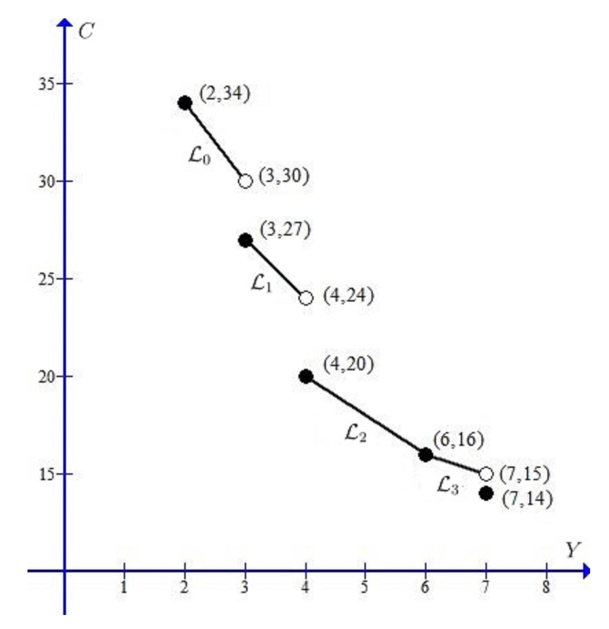
Let us consider the job instance $I_1$ displayed in Table 1. The trade-off curve of problem ${1\left|\mathrm{pmtn}\right|}^{\#}(\sum C_j^A,\sum Y_j^B)$ on instance $I_1$ is shown in Figure 1.

Table 1. The job instance $I_1$.

${\mathit{J}}_{\mathit{i}}^{\mathit{X}}$	${\mathit{J}}_1^{\mathit{A}}$	${\mathit{J}}_2^{\mathit{A}}$	${\mathit{J}}_3^{\mathit{A}}$	${\mathit{J}}_4^{\mathit{A}}$	${\mathit{J}}_1^{\mathit{B}}$	${\mathit{J}}_2^{\mathit{B}}$	${\mathit{J}}_3^{\mathit{B}}$
$p_i^X$	1	1	2	3	2	4	2
$d_i^X$	0	0	0	0	3	4	8

Figure 1. Trade-off curve.

Please note that $P^{*}=P+1=16$. Let $\mathsf{\Omega }=\mathsf{\Omega }({\mathcal{J}}^A,{\mathcal{J}}^B)$. The key steps in applying Algorithm 2 to solve the instance $I_1$ are as follows:

(i)

Generate the schedule ${\sigma }_0^B=(J_1^B,J_2^B,J_3^B)$ and calculate the Y-value $Y^{\left(0\right)}=T_{max}\left({\sigma }_0^B\right)=2$. Then generate the schedule ${\sigma }^{B\left(Y^{\left(0\right)}\right)}$, and the forbidden interval set ${\mathcal{I}}^{B\left(Y^{\left(0\right)}\right)}=\{h_1,h_2,h_3\}$ is determined, where $h_1=[0,4]$, $h_2=[6,8]$, and $h_3=[16,18]$. Then, for each $y\in (Y^{\left(0\right)},P_B]=(2,8]$, ${\sigma }^{B\left(y\right)}$ and ${\mathcal{I}}^{B\left(y\right)}$ can be easily generated.

(ii)

Generate the $Y^{\left(0\right)}$-standard schedule ${\sigma }_0$ of ${\mathcal{J}}^A\cup {\mathcal{J}}^B$ in which $h_1,h_2,h_3$ are the forbidden intervals and the A-jobs are preemptively scheduled in the order $J_1^A\prec J_2^A\prec J_3^A\prec J_4^A$ as early as possible. Determine the value $C^{\left(0\right)}={\sum }_{j=1}^{n_A}{C}_j^A\left({\sigma }_0\right)=34$. Then ${\sigma }_0$ is a Pareto-optimal schedule corresponding to $(34,2)\in \mathsf{\Omega }$.

(iii)

Calculate the values $k\left({\sigma }_0\right)=1$ and $\theta \left({\sigma }_0\right)=1$. Then line segment ${\mathcal{L}}_0$, which is the trade-off curve in the interval $[2,3)$, satisfies $C=-4Y+42$. Calculate $Y^{\left(1\right)}=Y^{\left(0\right)}+\theta \left({\sigma }_0\right)=3$ and the forbidden interval set ${\mathcal{I}}^{B\left(Y^{\left(1\right)}\right)}=\{h_1,h_2,h_3\}$, where $h_1=[1,4]$, $h_2=[6,8]$, and $h_3=[16,19]$. Generate ${\sigma }_1$, and calculate $C^{\left(1\right)}={\sum }_{j=1}^{n_A}{C}_j^A\left({\sigma }_1\right)=27$. Then the intermediate point $(27,3)\in \mathsf{\Omega }$ is a jump discontinuity point and ${\sigma }_1$ is a Pareto-optimal schedule corresponding to $(27,3)$.

(iv)

Calculate the values $k\left({\sigma }_1\right)=2$ and $\theta \left({\sigma }_1\right)=1$. Then the line segment ${\mathcal{L}}_1$, which is the trade-off curve in the interval $[3,4)$, satisfies $C=-3Y+36$. Calculate $Y^{\left(2\right)}=Y^{\left(1\right)}+\theta \left({\sigma }_1\right)=4$ and the forbidden interval set ${\mathcal{I}}^{B\left(Y^{\left(2\right)}\right)}=\{h_1,h_2,h_3\}$, where $h_1=[2,4]$, $h_2=[6,8]$, and $h_3=[16,20]$. Generate ${\sigma }_2$, and calculate $C^{\left(2\right)}={\sum }_{j=1}^{n_A}{C}_j^A\left({\sigma }_2\right)=20$. Then the intermediate point $(20,4)\in \mathsf{\Omega }$ is a jump discontinuity point and ${\sigma }_2$ is a Pareto-optimal schedule corresponding to $(20,4)$.

(v)

Calculate the values $k\left({\sigma }_2\right)=3$ and $\theta \left({\sigma }_2\right)=2$. Then the line segment ${\mathcal{L}}_2$, which is the trade-off curve in the interval $[4,6)$, satisfies $C=-2Y+28$. Calculate $Y^{\left(3\right)}=Y^{\left(2\right)}+\theta \left({\sigma }_2\right)=6$ and the forbidden interval set ${\mathcal{I}}^{B\left(Y^{\left(3\right)}\right)}=\{h_2,h_3\}$, where $h_2=[6,8]$ and $h_3=[16,22]$. Generate ${\sigma }_3$, and calculate $C^{\left(3\right)}={\sum }_{j=1}^{n_A}{C}_j^A\left({\sigma }_3\right)=16$. Then the intermediate point $(16,6)\in \mathsf{\Omega }$ is a break point and ${\sigma }_3$ is a Pareto-optimal schedule corresponding to $(16,6)$.

(vi)

Calculate the values $k\left({\sigma }_3\right)=4$ and $\theta \left({\sigma }_3\right)=1$. Then the line segment ${\mathcal{L}}_3$, which is the trade-off curve in the interval $[6,7)$, satisfies $C=-Y+22$. Calculate $Y^{\left(4\right)}=Y^{\left(3\right)}+\theta \left({\sigma }_3\right)=7$ and the forbidden interval set ${\mathcal{I}}^{B\left(Y^{\left(4\right)}\right)}=\{h_2,h_3\}$, where $h_2=[7,8]$ and $h_3=[16,23]$. Generate ${\sigma }_4$, and calculate $C^{\left(4\right)}={\sum }_{j=1}^{n_A}{C}_j^A\left({\sigma }_4\right)=14$. Then the intermediate point $(14,7)\in \mathsf{\Omega }$ is a jump discontinuity point and ${\sigma }_4$ is a Pareto-optimal schedule corresponding to $(14,7)$.

(vii)

Finally, we conclude that $\mathsf{\Omega }=\{{\mathcal{L}}_0\cup {\mathcal{L}}_1\cup {\mathcal{L}}_2\cup {\mathcal{L}}_3\cup \left\{(14,7)\right\}\}$ as displayed in Figure 1.

4. The Second Problem

In this section, we consider problem ${1\left|\mathrm{pmtn}\right|}^{\#}(L_{max}^A,\sum Y_j^B)$ on instance ${\mathcal{J}}^A\bigcup {\mathcal{J}}^B$. By the job-shifting argument, we can verify that for each Pareto-optimal point, there is a corresponding Pareto-optimal schedule in which the A-jobs are scheduled in the EDD order. Thus, in this section, we renumber the A-jobs by the EDD order such that $d_1^A\le d_2^A\le \cdots \le d_{n_A}^A$. Then we only consider the schedules in which the A-jobs are scheduled in the order $J_1^A\prec J_2^A\prec \cdots \prec J_{n_A}^A$.

For a point $(L^{*},Y^{*})\in \mathsf{\Omega }({\mathcal{J}}^A,{\mathcal{J}}^B)$, let $\sigma$ be a $Y^{*}$-standard schedule of ${\mathcal{J}}^A\cup {\mathcal{J}}^B$. Then the set of forbidden intervals (occupied by the B-jobs) is given by (5) and the A-jobs are preemptively scheduled in the order $J_1^A\prec J_2^A\prec \cdots \prec J_{n_A}^A$ from time 0 in the free-time intervals. Thus, there are $m-i^{*}+1$ forbidden intervals and the first forbidden interval in $\sigma$ is given by $h_{i^{*}}=[{\tau }^{*},{\tau }_2^{\left(i^{*}\right)}]$.

If $P_A\le {\tau }^{*}$, then all the A-jobs are scheduled before the first forbidden interval $h_{i^{*}}$ in $\sigma$. In this case, we have no further action.

In general, suppose that $P_A>{\tau }^{*}$. Then at least one A-job completing after $h_{i^{*}}$ in $\sigma$. Let $J_{k\left(\sigma \right)}^A$ be the first A-job which completes after $h_{i^{*}}$ in $\sigma$. Then, there are totally $n_A-k\left(\sigma \right)+1$A-jobs completing after $h_{i^{*}}$ in $\sigma$.

Let $L^{*}=L_{max}^A\left(\sigma \right)$ be the maximum lateness of A-jobs in $\sigma$. An A-job $J_j^A$ with $k\left(\sigma \right)\le j\le n_A$ is called critical in $\sigma$ if $L_j^A\left(\sigma \right)=L_{max}^A\left(\sigma \right)$. Again, we use ${\mathcal{J}}_c^A\left(\sigma \right)$ to denote the set of all critical A-jobs. Then ${\mathcal{J}}_c^A\left(\sigma \right)=\{J_j^A:L_j^A\left(\sigma \right)=L^{*},k\left(\sigma \right)\le j\le n_A\}$.

For each critical A-job $J_j^A$, we define $i\left[j\right]$ to be the interval index such that $J_j^A$ completes after interval $h_{i\left[j\right]}$ and before interval $h_{i\left[j\right]+1}$ in $\sigma$, or equivalently, ${\tau }_2^{\left(i\right[j\left]\right)}<C_j^A\left(\sigma \right)\le {\tau }_1^{\left(i\right[j]+1)}$. Define

$$\lambda \left(\sigma \right)=max\{C_j^A\left(\sigma \right)-{\tau }_2^{\left(i\right[j\left]\right)}:J_j^A\in {\mathcal{J}}_c^A\left(\sigma \right)\}.$$

(9)

A critical A-job $J_j^A$ is called a desired A-job in $\sigma$ if $C_j^A\left(\sigma \right)-{\tau }_2^{\left(i\right[j\left]\right)}=\lambda \left(\sigma \right)$. In this case, interval $h_{i\left[j\right]}$ is called the nearest forbidden interval corresponding to desired A-job $J_j^A$ in $\sigma$. We further define

$$BL\left(\sigma \right)=max\{L_j^A\left(\sigma \right):C_j^A\left(\sigma \right)\le {\tau }^{*}\},$$

(10)

and

$$\Delta \left(\sigma \right)=L^{*}-BL\left(\sigma \right).$$

(11)

In the case that no A-job completes before interval $h_{i^{*}}$, we define $BL\left(\sigma \right)=-\infty$ and $\Delta \left(\sigma \right)=+\infty$. Moreover, we define

$$\vartheta \left(\sigma \right)=min\{min\{\lambda \left(\sigma \right),{\delta }_{i^{*}}\left(\sigma \right)\},\Delta \left(\sigma \right)\}.$$

(12)

Please note that when the schedule $\sigma$ is given, the values $C_j^A\left(\sigma \right)$ and $L_j^A\left(\sigma \right)$, $j=1,2,\dots ,n_A$, and $L^{*}$ can be determined in $O\left(n_A\right)$ time. Then the set ${\mathcal{J}}_c^A\left(\sigma \right)$ and the interval indices $i\left[j\right]$ for $J_j^A\in {\mathcal{J}}_c^A\left(\sigma \right)$ can be determined in $O\left(n_A\right)$ time. After that, the value $\lambda \left(\sigma \right)$, $BL\left(\sigma \right)$ and $\Delta \left(\sigma \right)$ can be determined in $O\left(n_A\right)$ time. Finally, the value $\vartheta \left(\sigma \right)$ can be determined by its definition in (12) in constant time. Then we have the following lemma.

Lemma 6.

Given the $Y^{*}$-standard schedule σ in advance, the values $\Delta \left(\sigma \right)$ and $\vartheta \left(\sigma \right)$ can be determined in $O\left(n_A\right)$ time.

If $\Delta \left(\sigma \right)=0$, then $BL\left(\sigma \right)=L^{*}$. In this case, $(L^{*},Y^{*})$ is the last Pareto-optimal point.

Suppose that $\Delta \left(\sigma \right)>0$. Then $\vartheta \left(\sigma \right)>0$. For each $Y\in [Y^{*},Y^{*}+\vartheta \left(\sigma \right)]$, let ${\sigma }^{\prime }$ be the Y-standard schedule. Then ${\sigma }^{\prime }$ is obtained from $\sigma$ by shifting $Y-Y^{*}$ units of $h_{i^{*}}$ to the last forbidden interval and then moving the A-jobs in $\{J_{k\left(\sigma \right)}^A,J_{k\left(\sigma \right)+1}^A,\dots ,J_{n_A}\}$ left to eliminate the idle times accordingly. This means that $L_j^A\left({\sigma }^{\prime }\right)\le L_j^A\left(\sigma \right)-(Y-Y^{*})$ for $j\in \{k\left(\sigma \right),k\left(\sigma \right)+1,\dots ,n_A\}$. Assume that the maximum lateness of A-jobs in ${\sigma }^{\prime }$ is L. According to Lemma 2, $(L,Y)$ is a Pareto-optimal point. In the following, we consider the trade-off curve between $(L^{*},Y^{*})$ and $(L,Y)$. For convenience, point $(L,Y)$ is simply called point Y.

We will show that the trade-off curve for $Y\in [Y^{*},Y^{*}+\vartheta \left(\sigma \right))$ is a line segment. Discussion for the singularity of the point $Y^{*}+\vartheta \left(\sigma \right)$ will be omitted. This does not affect the characterization of the trade-off curve.

Lemma 7.

Suppose that $\Delta \left(\sigma \right)>0$. For each point $(L,Y)\in \mathsf{\Omega }({\mathcal{J}}^A,{\mathcal{J}}^B)$ with $Y\in [Y^{*},Y^{*}+\vartheta \left(\sigma \right))$, we have $\frac{L-L^{*}}{Y-Y^{*}}=-1$.

Proof. 

For each $Y\in [Y^{*},Y^{*}+\vartheta \left(\sigma \right))$, we have $Y-Y^{*}<\vartheta \left(\sigma \right)$. When we change $\sigma$ to ${\sigma }^{\prime }$, no desired A-jobs are moved left across their corresponding nearest forbidden intervals in ${\sigma }^{\prime }$. As a result, compared with $\sigma$, each desired job must move forward $Y-Y^{*}$ units and the other A-jobs move forward at least $Y-Y^{*}$ units in ${\sigma }^{\prime }$. Thus, the desired A-jobs in $\sigma$ are also critical A-jobs in ${\sigma }^{\prime }$. Then we have $\frac{L-L^{*}}{Y-Y^{*}}=-1$, as required. □

Theorem 2.

Algorithm 3 generates the trade-off curve of ${1\left|pmtn\right|}^{\#}(L_{max}^A,\sum Y_j^B)$ in $O\left(n{n}_A{n}_B\right)$ time.

Algorithm 3: Trade-off curve of problem ${1\left|\mathrm{pmtn}\right|}^{\#}(L_{max}^A,\sum Y_j^B)$.

Input: Instance ${\mathcal{J}}^A\cup {\mathcal{J}}^B$.

Preprocessing: Renumber the A-jobs such that $d_1^A\le d_2^A\le \cdots \le d_{n_A}^A$ and renumber the B-jobs such that $d_1^B\le d_2^B\le \cdots \le d_{n_B}^B$.

Step 1: Do the following:

(1.1) Generate schedule ${\sigma }_0^B$ which schedules the B-jobs in the order $J_1^B\prec J_2^B\prec \cdots \prec J_{n_B}^B$ in the interval $[0,P_B]$ without idle times. Then calculate the value $Y^{\left(0\right)}=T_{max}\left({\sigma }_0^B\right)$.

(1.2) Run Procedure($Y^{\left(0\right)}$) to obtain the schedule ${\sigma }^{B\left(Y^{\left(0\right)}\right)}$ of the B-jobs. Determine the intervals occupied by the B-jobs in ${\sigma }^{B\left(Y^{\left(0\right)}\right)}$, say $h_1,h_2,\dots ,h_m$, where $h_i=[{\tau }_1^{\left(i\right)},{\tau }_2^{\left(i\right)}]$ is the i-th interval, $i=1,2,\dots ,m$, as described in (3). Then regard $h_1,h_2,\dots ,h_m$ as forbidden intervals which will be updated in the implementation of the algorithm. We take the convention that the forbidden intervals are just occupied by the B-jobs.

(1.3) Set $t_0:=1$ and set $i:=0$.

Step 2: Do the following:

(2.1) Generate the $Y^{\left(i\right)}$-standard schedule ${\sigma }_i$ of ${\mathcal{J}}^A\cup {\mathcal{J}}^B$ in which $h_{t_i},h_{t_i+1},\dots ,h_m$ are the forbidden intervals and the A-jobs are preemptively scheduled in the order $J_1^A\prec J_2^A\prec \cdots \prec J_{n_A}^A$ as early as possible. Determine the values $L^{\left(i\right)}=L_{max}^A\left({\sigma }_i\right)$.

(2.2) Determine the value $\Delta \left({\sigma }_i\right)$. Moreover, if $\Delta \left({\sigma }_i\right)>0$, determine the value $\vartheta \left({\sigma }_i\right)$.

(2.3) If $\Delta \left({\sigma }_i\right)=0$, then set $K=i$ and go to Step 4. (In this case, we have obtained the whole trade-off curve.)

If $\Delta \left({\sigma }_i\right)>0$, then go to Step 3. (In this case, we have $\vartheta \left({\sigma }_i\right)>0$.)

Step 3: Define a left closed right open segment ${\mathcal{L}}_i$ in the interval $[Y^{\left(i\right)},Y^{\left(i\right)}+\vartheta \left({\sigma }_i\right))$ by the following way: $${\mathcal{L}}_i:\frac{L-L^{\left(i\right)}}{Y-Y^{\left(i\right)}}=-1,Y\in [Y^{\left(i\right)},Y^{\left(i\right)}+\vartheta \left({\sigma }_i\right)).$$

(3.3) Set $Y^{(i+1)}:=Y^{\left(i\right)}+\vartheta \left({\sigma }_i\right)$ and $h_m:=[P^{*},P^{*}+Y^{(i+1)}]$. Moreover, if $\vartheta \left({\sigma }_i\right)={\delta }_{t_i}\left({\sigma }_i\right)$, then set $t_{i+1}:=t_i+1$; and if $\vartheta \left({\sigma }_i\right)<{\delta }_{t_i}\left({\sigma }_i\right)$, then set $t_{i+1}:=t_i$ and $h_{t_{i+1}}:=[{\tau }_1^{\left(t_i\right)}+\vartheta \left({\sigma }_i\right),{\tau }_2^{\left(t_i\right)}]$ (which is obtained from interval $h_{t_i}$ by deleting the first $\vartheta \left({\sigma }_i\right)$ units.)

(3.4) Set $i:=i+1$. Go to Step 2.

Step 4: Output the trade-off curve $\mathsf{\Omega }({\mathcal{J}}^A,{\mathcal{J}}^B)={\mathcal{L}}_0\cup {\mathcal{L}}_1\cup \cdots \cup {\mathcal{L}}_{K-1}\cup \left\{(L^{\left(K\right)},Y^{\left(K\right)})\right\}$.

Proof. 

Correctness of Algorithm 3 is guaranteed by Lemmas 2 and 7. The time complexity can be estimated by the similar way of Theorem 1 by putting Lemma 6 in discussion. □

It can be observed that the total interruption time (i.e., the number of interruptions) of all the jobs in each schedule generated by Algorithm 3 is upper bounded by $1+m\le 1+n_B$.

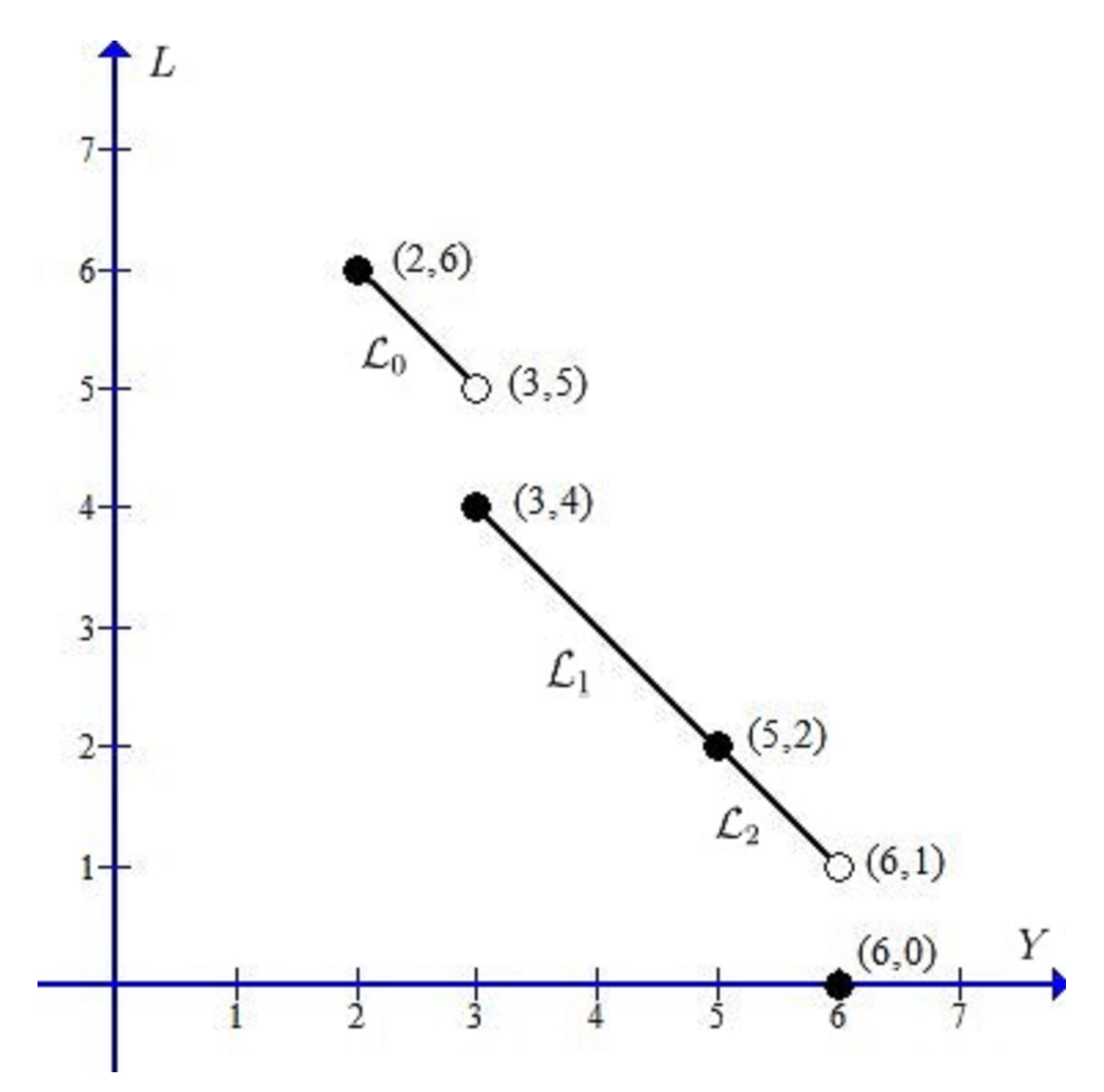
Let us consider the job instance $I_2$ displayed in Table 2. The trade-off curve of problem ${1\left|\mathrm{pmtn}\right|}^{\#}(L_{max}^A,\sum Y_j^B)$ on instance $I_2$ is shown in Figure 2.

Table 2. The instance $I_2$.

${\mathit{J}}_{\mathit{i}}^{\mathit{X}}$	${\mathit{J}}_1^{\mathit{A}}$	${\mathit{J}}_2^{\mathit{A}}$	${\mathit{J}}_3^{\mathit{A}}$	${\mathit{J}}_1^{\mathit{B}}$	${\mathit{J}}_2^{\mathit{B}}$	${\mathit{J}}_3^{\mathit{B}}$
$p_i^X$	4	2	3	5	2	2
$d_i^X$	4	7	11	3	7	12

Figure 2. Trade-off curve.

Please note that $P^{*}=P+1=19$. Let $\mathsf{\Omega }=\mathsf{\Omega }({\mathcal{J}}^A,{\mathcal{J}}^B)$. The key steps in applying Algorithm 3 to solve the instance $I_2$ are as follows:

(i)

Generate the schedule ${\sigma }_0^B=(J_1^B,J_2^B,J_3^B)$ and calculate the Y-value $Y^{\left(0\right)}=T_{max}\left({\sigma }_0^B\right)=2$. Then generate the schedule ${\sigma }^{B\left(Y^{\left(0\right)}\right)}$, and the forbidden interval set ${\mathcal{I}}^{B\left(Y^{\left(0\right)}\right)}=\{h_1,h_2,h_3,h_4\}$ is determined, where $h_1=[0,3]$, $h_2=[5,7]$, $h_3=[10,12]$, and $h_4=[19,21]$. Then, for each $y\in (Y^{\left(0\right)},P_B]=(2,9]$, ${\sigma }^{B\left(y\right)}$ and ${\mathcal{I}}^{B\left(y\right)}$ can be easily generated.

(ii)

Generate the $Y^{\left(0\right)}$-standard schedule ${\sigma }_0$ of ${\mathcal{J}}^A\cup {\mathcal{J}}^B$ in which $h_1,h_2,h_3,h_4$ are the forbidden intervals and the A-jobs are preemptively scheduled in the order $J_1^A\prec J_2^A\prec J_3^A$ as early as possible. Determine the value $L^{\left(0\right)}=L_{max}^A\left({\sigma }_0\right)=6$. Then ${\sigma }_0$ is a Pareto-optimal schedule corresponding to $(6,2)\in \mathsf{\Omega }$.

(iii)

Calculate the values $\Delta \left({\sigma }_0\right)=6>0$ and $\vartheta \left({\sigma }_0\right)=1$. Then the line segment ${\mathcal{L}}_0$, which is the trade-off curve in the interval $[2,3)$, satisfies $L=-Y+8$. Calculate $Y^{\left(1\right)}=Y^{\left(0\right)}+\vartheta \left({\sigma }_0\right)=3$ and the forbidden interval set ${\mathcal{I}}^{B\left(Y^{\left(1\right)}\right)}=\{h_1,h_2,h_3,h_4\}$, where $h_1=[1,3]$, $h_2=[5,7]$, $h_3=[10,12]$, and $h_4=[19,22]$. Generate ${\sigma }_1$, and calculate $L^{\left(1\right)}=L_{max}^A\left({\sigma }_1\right)=4$. Then the intermediate point $(4,3)\in \mathsf{\Omega }$ is a jump discontinuity point and ${\sigma }_1$ is a Pareto-optimal schedule corresponding to $(4,3)$.

(iv)

Calculate the values $\Delta \left({\sigma }_1\right)=4>0$ and $\vartheta \left({\sigma }_1\right)=2$. Then the line segment ${\mathcal{L}}_1$, which is the trade-off curve in the interval $[3,5)$, satisfies $L=-Y+7$. Calculate $Y^{\left(2\right)}=Y^{\left(1\right)}+\vartheta \left({\sigma }_1\right)=5$ and the forbidden interval set ${\mathcal{I}}^{B\left(Y^{\left(2\right)}\right)}=\{h_2,h_3,h_4\}$, where $h_2=[5,7]$, $h_3=[10,12]$, and $h_4=[19,24]$. Generate ${\sigma }_2$, and calculate $L^{\left(2\right)}=L_{max}^A\left({\sigma }_2\right)=2$. Then the intermediate point $(2,5)\in \mathsf{\Omega }$ is a continuity point and ${\sigma }_2$ is a Pareto-optimal schedule corresponding to $(2,5)$.

(v)

Calculate the values $\Delta \left({\sigma }_2\right)=2>0$ and $\vartheta \left({\sigma }_2\right)=1$. Then the line segment ${\mathcal{L}}_2$, which is the trade-off curve in the interval $[5,6)$, satisfies $L=-Y+7$. Calculate $Y^{\left(3\right)}=Y^{\left(2\right)}+\vartheta \left({\sigma }_2\right)=6$ and the forbidden interval set ${\mathcal{I}}^{B\left(Y^{\left(2\right)}\right)}=\{h_2,h_3,h_4\}$, where $h_2=[6,7]$, $h_3=[10,12]$, and $h_4=[19,25]$. Generate ${\sigma }_3$, and calculate $L^{\left(3\right)}=L_{max}^A\left({\sigma }_3\right)=0$. Then the intermediate point $(0,6)\in \mathsf{\Omega }$ is a jump discontinuity point and ${\sigma }_3$ is a Pareto-optimal schedule corresponding to $(0,6)$.

(vi)

Calculate the value $\Delta \left({\sigma }_3\right)=0$. Then, we conclude that $\mathsf{\Omega }=\{{\mathcal{L}}_0\cup {\mathcal{L}}_1\cup {\mathcal{L}}_2\cup \left\{(0,6)\right\}\}$ as displayed in Figure 2.

5. The Third Problem

In this section, we consider problem ${1\left|\mathrm{pmtn}\right|}^{\#}(\sum Y_j^A,\sum Y_j^B)$ on instance ${\mathcal{J}}^A\cup {\mathcal{J}}^B$. We renumber the A-jobs by the EDD order such that $d_1^A\le d_2^A\le \cdots \le d_{n_A}^A$.

For a point $(Y^A,Y^B)\in \mathsf{\Omega }({\mathcal{J}}^A,{\mathcal{J}}^B)$, a $Y^B$-standard schedule of ${\mathcal{J}}^A\cup {\mathcal{J}}^B$ corresponding to $(Y^A,Y^B)$ can be obtained in the following way in $O\left(n\right)$ time: (i) Run Procedure($Y^B$) to obtain the schedule ${\sigma }^{B\left(Y^B\right)}$ of the B-jobs, and (ii) run the algorithm in Hariri et al. [21] for solving problem $1\left|\mathrm{pmtn}\right|\sum Y_j$ to schedule the A-jobs in the free-time intervals not occupied by the B-jobs in ${\sigma }^{B\left(Y^B\right)}$. Thus, we only need to consider the trade-off curve of problem ${1\left|\mathrm{pmtn}\right|}^{\#}(\sum Y_j^A,\sum Y_j^B)$ on instance ${\mathcal{J}}^A\cup {\mathcal{J}}^B$. We first establish a nice property for problem $1\left|\mathrm{pmtn}\right|\sum Y_j$ in the following lemma.

Lemma 8.

Let $\mathcal{J}=\{J_1,J_2,\dots ,J_n\}$ be a job instance of problem $1\left|pmtn\right|\sum Y_j$. Let $\mathcal{U}$ be a subset of $\mathcal{J}$ such that there is a schedule of instance $\mathcal{J}$ such that all the jobs in $\mathcal{U}$ are early. Then there is an optimal schedule of problem $1\left|pmtn\right|\sum Y_j$ on instance $\mathcal{J}$ such that all the jobs in $\mathcal{U}$ are early.

Proof. 

We first prove the result for problem $1\left|\mathrm{pmtn}\right|\sum Y_j$ without maintenance intervals by induction on $\left|\mathcal{U}\right|$. The result holds trivially if $\left|\mathcal{U}\right|=0$.

Inductively, suppose that $\left|\mathcal{U}\right|=k\ge 1$, $\mathcal{U}=\{J_{j_1},J_{j_2},\dots ,J_{j_k}\}$, $d_{j_1}\le d_{j_2}\le \cdots \le d_{j_k}$, and there is a feasible schedule of instance $\mathcal{J}$ such that all the jobs in $\mathcal{U}$ are early. Moreover, the result holds for every proper subset of $\mathcal{U}$ (the induction hypothesis).

Since $\mathcal{U}\backslash \left\{J_{j_k}\right\}$ is a proper subset of $\mathcal{U}$, from the induction hypothesis, there is an optimal schedule $\pi$ of problem $1\left|\mathrm{pmtn}\right|\sum Y_j$ on instance $\mathcal{J}$ such that all the $k-1$ jobs $J_{j_1},J_{j_2},\dots ,J_{j_{k-1}}$ are early in $\pi$. Since all the jobs in $\mathcal{U}$ are early in some feasible schedule, we have $p_{j_1}+p_{j_2}+\cdots +p_{j_k}\le max\{d_{j_1},d_{j_2},\dots ,d_{j_k}\}=d_{j_k}$. This implies that all the $k-1$ jobs $J_{j_1},J_{j_2},\dots ,J_{j_{k-1}}$ are completed by time $d_{j_k}$ in $\pi$ and at least $p_{j_k}$ units of time in the interval $[0,d_{j_k}]$ are not occupied by the $k-1$ jobs $J_{j_1},J_{j_2},\dots ,J_{j_{k-1}}$.

If $C_{j_k}\left(\pi \right)\le d_{j_k}$, i.e., $J_{j_k}$ is early in $\pi$, then $\pi$ is a required optimal schedule.

Suppose in the following that $C_{j_k}\left(\pi \right)>d_{j_k}$. Then there is a certain index $i\in \{0,1,\dots ,p_{j_k}\}$ such that for job $J_{j_k}$, the first i unit pieces $J_{j_k,1}\left(\pi \right),J_{j_k,2}\left(\pi \right),\dots ,J_{j_k,i}\left(\pi \right)$ are early in $\pi$ and the last $p_{j_k}-i$ unit pieces $J_{j_k,i+1}\left(\pi \right),\dots ,J_{j_k,p_{j_k}}\left(\pi \right)$ are late in $\pi$. Let $\mathcal{S}$ be the time space which consists of the last $p_{j_k}-i$ units of time in the interval $[0,d_{j_k}]$ that are not occupied by the $k-1$ jobs $J_{j_1},J_{j_2},\dots ,J_{j_{k-1}}$ and the i unit pieces $J_{j_k,1}\left(\pi \right),J_{j_k,2}\left(\pi \right),\dots ,J_{j_k,i}\left(\pi \right)$ of $J_{j_k}$. Let $\mathcal{T}$ be the time space which consists of the $p_{j_k}-i$ units of time that are occupied by the $p_{j_k}-i$ unit pieces $J_{j_k,i+1}\left(\pi \right),\dots ,J_{j_k,p_{j_k}}\left(\pi \right)$ of $J_{j_k}$. Let $\sigma$ be the schedule of $\mathcal{J}$ obtained from $\pi$ by exchanging the subschedules in $\mathcal{S}$ and in $\mathcal{T}$. Then $J_{j_k}$ is early in $\sigma$. Moreover, $\sum Y_j\left(\sigma \right)\le \sum Y_j\left(\pi \right)-\left|\mathcal{T}\right|+\left|\mathcal{S}\right|=\sum Y_j\left(\pi \right)$, implying that $\sigma$ is also optimal. Now all the jobs in $\mathcal{U}=\{J_{j_1},J_{j_2},\dots ,J_{j_k}\}$ are early in $\sigma$. Consequently, $\sigma$ is an optimal schedule of problem $1\left|\mathrm{pmtn}\right|\sum Y_j$ on instance $\mathcal{J}$ such that all the jobs in $\mathcal{U}$ are early. The result follows by the induction principle. □

We next use Lemma 8 to prove the following useful lemma.

Lemma 9.

Let $\mathcal{J}=\{J_1,J_2,\dots ,J_n\}$ be a job instance of problem $1\left|pmtn\right|\sum Y_j$. Let π be a schedule of the jobs in $\mathcal{J}$. Then there is an optimal schedule σ of problem $1\left|pmtn\right|\sum Y_j$ on instance $\mathcal{J}$ such that $Y_j\left(\sigma \right)\le Y_j\left(\pi \right)$ for $j=1,2,\dots ,n$.

Proof. 

For each $j\in \{1,2,\dots ,n\}$, we partition $J_j$ into two parts $J_{j^{\prime }}$ and $J_{j^{\prime \prime }}$ such that $p_{j^{\prime }}=p_j-Y_j\left(\pi \right)$ is the early work of $J_j$ in $\pi$, $p_{j^{\prime \prime }}=Y_j\left(\pi \right)$ is the late work of $J_j$ in $\pi$, and $d_{j^{\prime }}=d_{j^{\prime \prime }}=d_j$. Let ${\mathcal{J}}^{\prime }=\{J_{j^{\prime }},J_{j^{\prime \prime }}:j=1,2,\dots ,n\}$. Let ${\pi }^{\prime }$ be the schedule of ${\mathcal{J}}^{\prime }$ which is obtained from $\pi$ by just regarding the early part of $J_j$ in $\pi$ as job $J_{j^{\prime }}$ and regarding the late part of $J_j$ in $\pi$ as job $J_{j^{\prime \prime }}$. Then all the jobs in $\{J_{j^{\prime }}:j=1,2,\dots ,n\}$ are early in ${\pi }^{\prime }$. According to Lemma 8, there is an optimal schedule $\sigma$ of problem $1\left|\mathrm{pmtn}\right|\sum Y_j$ on instance ${\mathcal{J}}^{\prime }$ such that all the jobs in $\{J_{j^{\prime }}:j=1,2,\dots ,n\}$ are early. Since the preemptive assumption, the two instances $\mathcal{J}$ and ${\mathcal{J}}^{\prime }$ have no essential difference for problem $1\left|\mathrm{pmtn}\right|\sum Y_j$, $\sigma$ is an optimal schedule of problem $1\left|\mathrm{pmtn}\right|\sum Y_j$ on instance $\mathcal{J}$. The result follows by noting that $Y_j\left(\sigma \right)=Y_{j^{\prime \prime }}\left(\sigma \right)\le p_{j^{\prime \prime }}=Y_j\left(\pi \right)$ for $j=1,2,\dots ,n$. □

Let $Y^{AB}$ be the optimal value of problem $1\left|\mathrm{pmtn}\right|\sum Y_j$ on instance ${\mathcal{J}}^A\cup {\mathcal{J}}^B$. We have the following lemma.

Lemma 10.

For each point $(Y^A,Y^B)\in \mathsf{\Omega }({\mathcal{J}}^A,{\mathcal{J}}^B)$, we have $Y^A+Y^B=Y^{AB}$.

Proof. 

Let $\sigma$ be a Pareto-optimal schedule of problem ${1\left|\mathrm{pmtn}\right|}^{\#}(\sum Y_j^A,\sum Y_j^B)$ on instance ${\mathcal{J}}^A\cup {\mathcal{J}}^B$ such that $\sum Y_j^A\left(\sigma \right)=Y^A$ and $\sum Y_j^B\left(\sigma \right)=Y^B$. From Lemma 9, there is an optimal schedule ${\sigma }^{\prime }$ of $1\left|\mathrm{pmtn}\right|\sum Y_j$ on instance ${\mathcal{J}}^A\cup {\mathcal{J}}^B$ such that $\sum Y_j^A\left({\sigma }^{\prime }\right)\le \sum Y_j^A\left(\sigma \right)$ and $\sum Y_j^B\left({\sigma }^{\prime }\right)\le \sum Y_j^B\left(\sigma \right)$. The optimality of ${\sigma }^{\prime }$ implies that $\sum Y_j\left({\sigma }^{\prime }\right)=Y^{AB}$. From the property of Pareto-optimal point, we can obtain that $\sum Y_j^A\left({\sigma }^{\prime }\right)=\sum Y_j^A\left(\sigma \right)$ and $\sum Y_j^B\left({\sigma }^{\prime }\right)=\sum Y_j^B\left(\sigma \right)$. Thus, we have $Y^A+Y^B=Y^{AB}$. The result follows. □

Theorem 3.

The trade-off curve of problem ${1\left|pmtn\right|}^{\#}(\sum Y_j^A,\sum Y_j^B)$ on instance ${\mathcal{J}}^A\cup {\mathcal{J}}^B$ can be determined in $O(nlogn)$ time.

Proof. 

Let $Y_A^{\left(0\right)}$ be the optimal value of problem $1\left|\mathrm{pmtn}\right|Y_j^A$ on instance ${\mathcal{J}}^A$. Let $Y_B^{\left(0\right)}$ be the optimal value of problem $1\left|\mathrm{pmtn}\right|Y_j^B$ on instance ${\mathcal{J}}^B$. Recall that $Y^{AB}$ is the optimal value of problem $1\left|\mathrm{pmtn}\right|\sum Y_j$ on instance ${\mathcal{J}}^A\cup {\mathcal{J}}^B$. From Hariri et al. [21], $Y_A^{\left(0\right)}$, $Y_B^{\left(0\right)}$, and $Y^{AB}$ can be determined in $O(n_{A}log{n}_A)$ time, $O(n_{B}log{n}_B)$ time, and $O(nlogn)$ time, respectively.

Please note that $Y_A^{\left(0\right)}$ is the minimum total late work of A-jobs among all Pareto-optimal points and $Y_B^{\left(0\right)}$ is the minimum total late work of B-jobs among all Pareto-optimal points. Thus, from Lemma 10, the trade-off curve is the line segment

$$Y^A+Y^B=Y^{AB},Y_B^{\left(0\right)}\le Y^B\le Y^{AB}-Y_A^{\left(0\right)},$$

connecting point $(Y^{AB}-Y_B^{\left(0\right)},Y_B^{\left(0\right)})$ to point $(Y_A^{\left(0\right)},Y^{AB}-Y_A^{\left(0\right)})$. So, the overall complexity to obtain the trade-off curve is given by $O(nlogn)$. □

It can be observed that the total interruption time (i.e., the number of interruptions) of all the jobs in each Pareto-optimal schedule is upper bounded by $max\{n_A,n_B\}+2$.

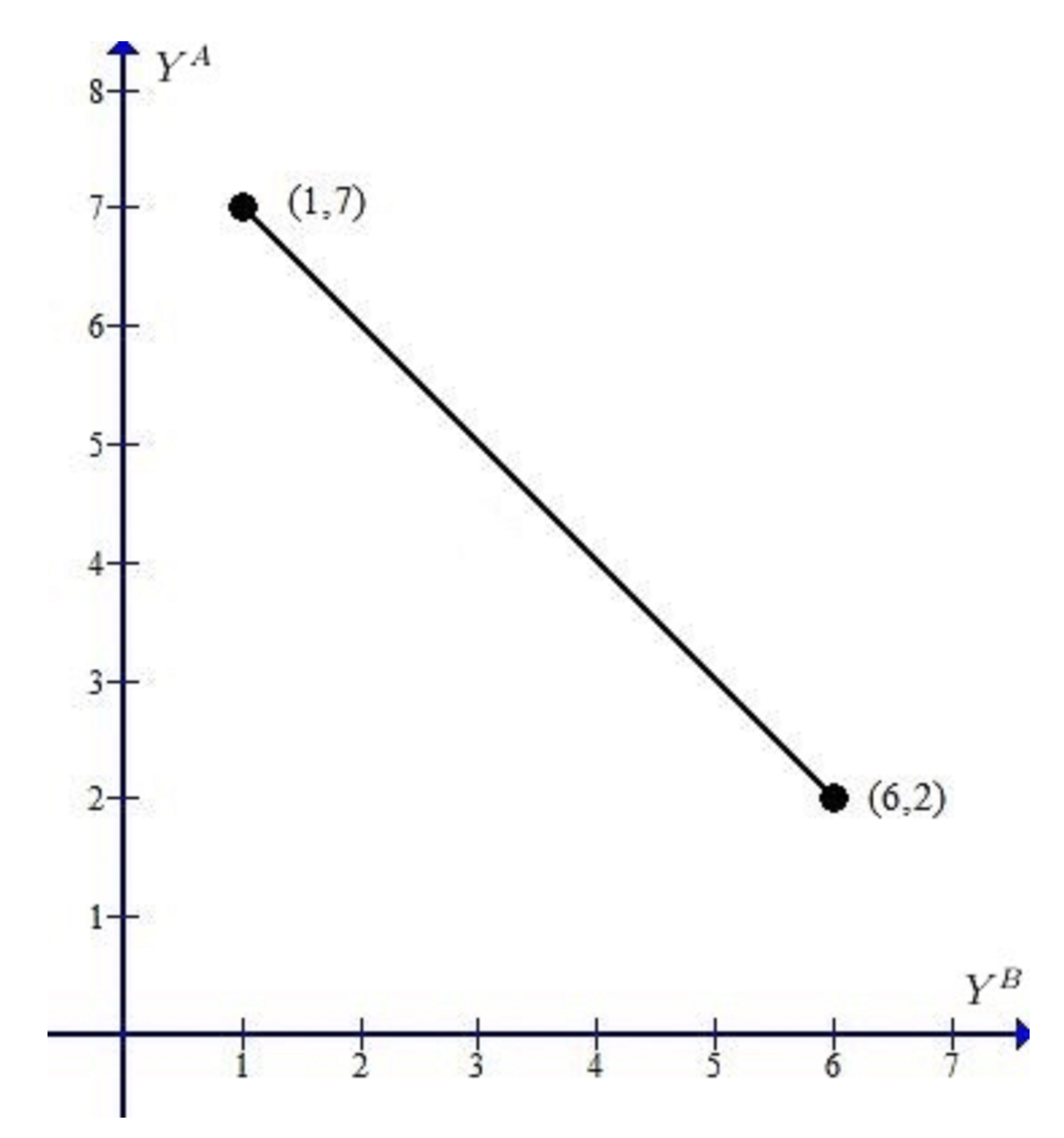
Let us consider the job instance $I_3$ displayed in Table 3. The trade-off curve of problem ${1\left|\mathrm{pmtn}\right|}^{\#}(\sum Y_j^A,\sum Y_j^B)$ on instance $I_3$ is shown in Figure 3.

Table 3. The instance $I_3$.

${\mathit{J}}_{\mathit{i}}^{\mathit{X}}$	${\mathit{J}}_1^{\mathit{A}}$	${\mathit{J}}_2^{\mathit{A}}$	${\mathit{J}}_3^{\mathit{A}}$	${\mathit{J}}_4^{\mathit{A}}$	${\mathit{J}}_5^{\mathit{A}}$	${\mathit{J}}_1^{\mathit{B}}$	${\mathit{J}}_2^{\mathit{B}}$	${\mathit{J}}_3^{\mathit{B}}$
$p_i^X$	4	2	3	2	2	3	3	3
$d_i^X$	3	4	7	11	14	2	8	13

Figure 3. Trade-off curve.

Please note that $P^{*}=P+1=23$. Let $\mathsf{\Omega }=\mathsf{\Omega }({\mathcal{J}}^A,{\mathcal{J}}^B)$. The key steps to solve the instance $I_3$ are as follows:

(i)

Generate the schedule ${\sigma }_0^B=(J_1^B,J_2^B,J_3^B)$ and calculate the $Y^B$-value $Y^{\left(0\right)}=T_{max}\left({\sigma }_0^B\right)=1$. Then generate the schedule ${\sigma }^{B\left(Y^{\left(0\right)}\right)}$, and the forbidden interval set ${\mathcal{I}}^{B\left(Y^{\left(0\right)}\right)}=\{h_1,h_2,h_3,h_4\}$ is determined, where $h_1=[0,2]$, $h_2=[5,8]$, $h_3=[10,13]$, and $h_4=[23,24]$. Then, for each $y\in (Y^{\left(0\right)},P_B]=(1,9]$, ${\sigma }^{B\left(y\right)}$ and ${\mathcal{I}}^{B\left(y\right)}$ can be easily generated.

(ii)

Generate the $Y^{\left(0\right)}$-standard schedule ${\sigma }_0$ of ${\mathcal{J}}^A\cup {\mathcal{J}}^B$ in which $h_1,h_2,h_3,h_4$ are the forbidden intervals and the A-jobs are preemptively scheduled by running the algorithm in Hariri et al. [21] for solving problem $1\left|\mathrm{pmtn}\right|\sum Y_j$ in the free-time intervals not occupied by the B-jobs in ${\sigma }^{B\left(Y^0\right)}$. Determine the value $Y^A\left({\sigma }_0\right)=\sum Y_j^A\left({\sigma }_0\right)=7$. Then ${\sigma }_0$ is a Pareto-optimal schedule corresponding to $(7,1)\in \mathsf{\Omega }$.

(iii)

By using the same method as (i) and (ii), we schedule A-jobs first. Generate the schedule ${\sigma }^{A\left(Y^{\left(0\right)}\right)}$, where $Y^{\left(0\right)}=T_{max}\left({\sigma }_0^A\right)=2$. Generate the schedule ${\sigma }_1$ of ${\mathcal{J}}^A\cup {\mathcal{J}}^B$ in which the B-jobs are preemptively scheduled by running the algorithm in Hariri et al. [21] for solving problem $1\left|\mathrm{pmtn}\right|\sum Y_j$ in the free-time intervals not occupied by the A-jobs in ${\sigma }^{A\left(Y^{\left(0\right)}\right)}$. Then ${\sigma }_1$ is a Pareto-optimal schedule corresponding to $(2,6)\in \mathsf{\Omega }$. From Lemma 10, ${\sigma }_1$ is the final Pareto-optimal schedule. Then the trade-off curve is just the line segment in the interval $[1,6]$, which satisfies $Y^A=-Y^B+8$ as displayed in Figure 3.

6. Conclusions

This paper considers three preemptive Pareto-scheduling problems with two competing agents on a single machine. Two agents compete to perform their respective jobs on a common single machine and each agent has his own criterion to optimize. In each problem, the goal of agent A is to minimize the total completion time, the maximum lateness, or the total late work while agent B wants to minimize the total late work. For each problem, we provide a polynomial-time algorithm to characterize the trade-off curve of all Pareto-optimal points.

Late-work criterion can be met in all cases where the penalty imposed on a solution depends on the number of tardy units of jobs performed in a system. For example, in production planning where the manufacturer is concerned with minimizing any order delays which cause financial loss, in control systems where the accuracy of control procedures depends on the amount of information provided as their input, in agriculture where performance measures based on due dates, and so on. In the case where two criteria need to be minimized, the trade-off curve results an ideal solution. Once the trade-off curve is characterized, decision makers can make decisions as needed.

For the future research, the trade-off curve of the problem ${1\left|\mathrm{pmtn}\right|}^{\#}(\sum C_j^A,\sum w_j{Y}_j^B)$ or ${1\left|\mathrm{pmtn}\right|}^{\#}(L_{max}^A,\sum w_j{Y}_j^B)$ is worthy of study. Since the existence of precedence constraints on scheduling problems reflects real-life problems, it is also worthy to study the two-agent problems with precedence constraints. Another interesting future research direction is to investigate fairness issues when the total late work is one of the criteria in two-agent scheduling problems.