On the Optimal Control of a Malware Propagation Model

Abstract

An important way considered to control malware epidemic processes is to take into account security measures that are associated to the systems of ordinary differential equations that governs the dynamics of such systems. We can observe two types of control measures: the analysis of the basic reproductive number and the study of control measure functions. The first one is taken at the beginning of the epidemic process and, therefore, we can consider this to be a prevention measure. The second one is taken during the epidemic process. In this work, we use the theory of optimal control that is associated to systems of ordinary equations in order to find a new function to control malware epidemic through time. Specifically, this approach is evaluate on a particular compartmental malware model that considers carrier devices.

1. Introduction

Nowadays, malware is one of the most important threats to security of information. The study and analysis of mathematical models to simulate malware propagation is an important task. In this sense, several mathematical models to study malware propagation have appeared in the scientific literature (see, for example, [1,2,3,4,5,6,7,8,9,10,11]). These are compartmental models that, in most cases, are based in differential ordinary equations (as a consequence, they are deterministic and global models). Usually, each model exhibits two equilibrium points: a disease free-equilibrium point and an epidemic equilibrium point. The qualitative study of the systems shows that the basic reproductive number $R_0$ plays a fundamental role in the analysis of the convergence of the system to one of these equilibrium points. Therefore, by analyzing the $R_0$, one could consider control measures at the beginning of the malware epidemic outbreak in order to determinate the evolution of the solutions and the final equilibrium reached. On the other hand, using control theory, we can find a suitable function to control the epidemic process. This function is part of the system and we can observe its influence through time (that is, we are able to control the epidemic during the time t).

The theory of the optimal control is a classical theory [12,13] that has several applications in Economy, Epidemiology, etc. [14]. This theory allows for one to obtain the solutions of a system of ordinary differential equations under some conditions by finding the minimum cost of some parameters and variables that are controlled. Therefore less control measures can be used considering this method. This problem is tackled by means of the maximum Pontryagin Principle. In this principle, several hypothesis and formulations are introduced with the aim to calculate a function to simulate these control measures. Moreover, it is possible to define the equations of the new control model taking this optimal function into account.

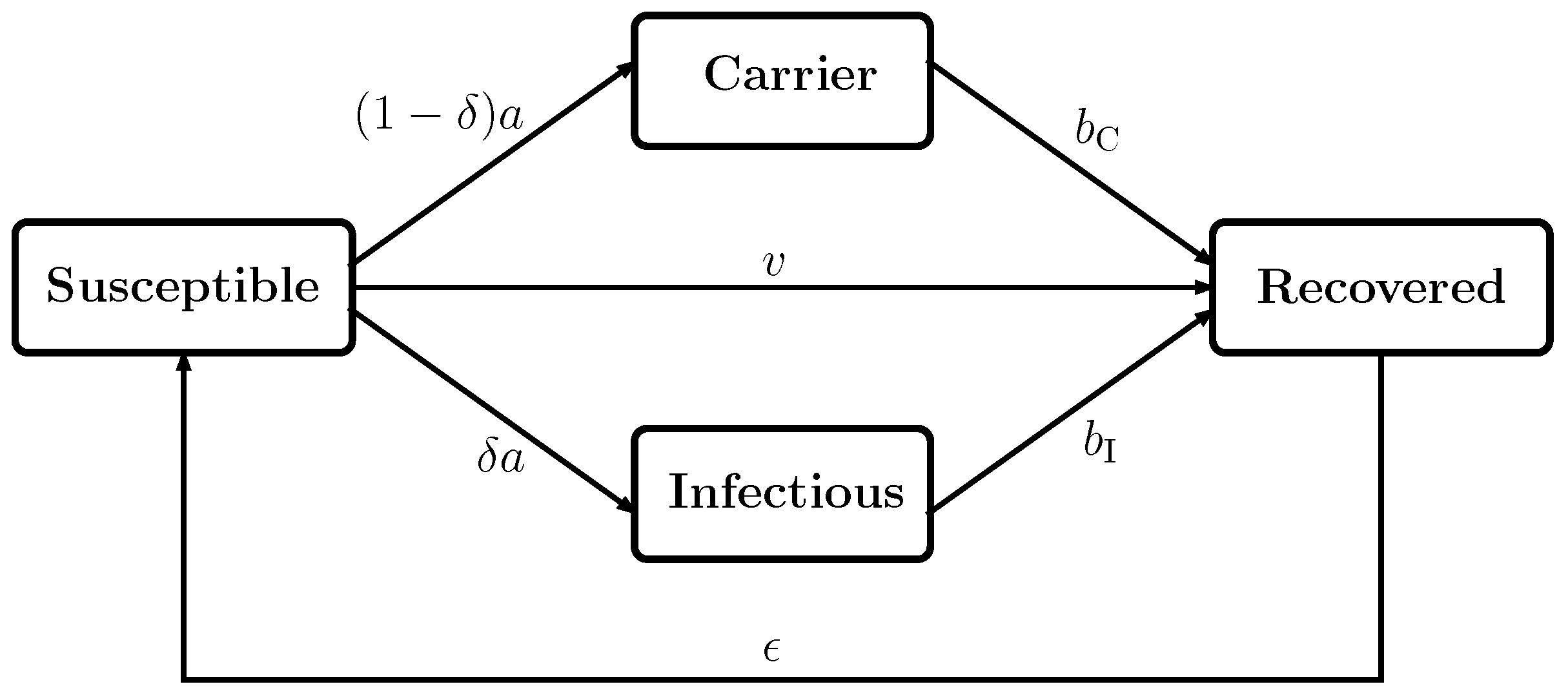
This approach is also used when malware propagation models are studied. Usually, compartmental models are proposed and analyzed; that is, the devices are classified into different compartments depending on their status with respect to malware -susceptible S, infectious I, exposed E, recovered R, etc. The dynamics between different compartments are ruled by means of epidemiological coefficients and, in this sense, several types of models can be proposed while taking into account the evolution of such compartments: SIR (Susceptible-Infectious-Recovered), etc. For example, in [15], a vaccination strategy to determine the optimal control is presented. In [8], two types of compartments are considered to construct the functional objective: the latent devices and breaking out devices. In [5] an analysis in order to minimize the infectious and dead devices through a optimal control is introduced. In [9], it is used the infectious devices and a delitescent strategy to remove the malware. In [1,4,6,7,10,13], the optimal control is calculated based on a $SIR$ model. In [11], the theory of control is used in a $S{I}_1{I}_{2}R$ model. In [3], it is presented the optimal control of a $SAI$ model. In [2], it is studied a control strategy of a $S\tilde{S}I\tilde{I}R\tilde{R}D$ model.

Furthermore, there exists several malware environments where this theory is used: in [1], this theory is used to simulate malware in mobile ad hoc networks. In [2,5,6], it is used to simulate malware propagation in wireless sensor networks. In [3], it is presented a model taking into account an alert system. In [8], it is considered scale-free networks. In [10], it presented a information network to simulate malware.

In [16], a compartmental $SCIRS$ model for malware propagation was proposed and analyzed from a qualitative perspective. Furthermore, some control measures based in the analysis of the basic reproductive number were proposed. In this article, we focus on the use of control measures that are developed over the time t. We use the theory of optimal control to do this work in this article. This control measure is different in this occasion due to it affects the system over all time t. This permits to have a new control tool to combat malware epidemics and improve the security of computers.

In Section 2, the model compartmental model is reviewed. In Section 3, the basis of the control functions is shown. The optimization problem and its analysis are presented in Section 4. Section 5 is devoted to illustrate the theory with some simulations. Finally, Section 6 presents the conclusions.

2. Relations between the Equations to Prevention and the Equations to Control

2.1. Autonomous Model for Malware Propagation

In this section, we review the deterministic and global mathematical model that simulates malware propagation using carrier compartment presented in [16]. This model consider four compartments: susceptible devices $S\left(t\right)$, carrier devices $C\left(t\right)$, infectious devices $I\left(t\right)$, and recovered devices, $R\left(t\right)$. Constant population is considered: $S\left(t\right)+I\left(t\right)+C\left(t\right)+R\left(t\right)=N>0$, with $t>0$. Carrier are those devices that can be infected by malware, but the malicious code is not able to perform its payload due to some reasons—for example, the device is not running on the targeted OS—although they can serve as transmission vectors.

In this model, it is supposed that carrier and infectious devices can both infect susceptible devices by malware at rate a. The fraction of vulnerable susceptible devices endowed with the targeted operative systems that the malware can infect is given by $\delta$ and they become infected. Because of security countermeasures, susceptible devices can be temporally immunized at vaccination rate v. Carriers and infectious devices can recover due to the security measures: the rates $b_C$ and $b_I$ represent these rates, respectively. Recovered devices can lose their temporal immunity at rate $ϵ$ (in

Table 1. Parameters of the model.

Parameter	Description	Range
v	Vaccination rate	$(0,1)$
a	Transmission rate	$(0,1)$
$b_C$	Recovery rate of carriers	$(0,1)$
$b_I$	Recovery rate of infectious	$(0,1)$
$ϵ$	Rate of lose of immunity of recovered	$(0,1)$
$\delta$	Rate of fraction of devices based on the targeted OS	$(0,1)$

these coefficients are illustrated). As a consequence, the dynamic of the epidemic model is governed by the following system of ordinary differential equations:

$$\left\{\begin{array}{ccc}\dot{S}\left(t\right)\hfill & =\hfill & -aS\left(t\right)\left(I\left(t\right)+C\left(t\right)\right)-vS\left(t\right)+ϵR\left(t\right),\hfill \\ \dot{C}\left(t\right)\hfill & =\hfill & a(1-\delta )S\left(t\right)\left(I\left(t\right)+C\left(t\right)\right)-b_{C}C\left(t\right),\hfill \\ \dot{I}\left(t\right)\hfill & =\hfill & a\delta S\left(t\right)\left(I\left(t\right)+C\left(t\right)\right)-b_{I}I\left(t\right),\hfill \\ \dot{R}\left(t\right)\hfill & =\hfill & vS\left(t\right)+b_{C}C\left(t\right)+b_{I}I\left(t\right)-ϵR\left(t\right),\hfill \end{array}\right.$$

(1)

Figure 1 shows the compartmental transition diagram of the dynamic model.

As $S\left(t\right)+I\left(t\right)+C\left(t\right)+R\left(t\right)=N$, we can simplify the system of ordinary differential equations, as follows:

$$\left\{\begin{array}{ccc}\dot{S}\left(t\right)\hfill & =\hfill & -aS\left(t\right)\left(I\left(t\right)+C\left(t\right)\right)-vS\left(t\right)+ϵ\left((N-S(t)-C(t)-I(t)\right),\hfill \\ \dot{C}\left(t\right)\hfill & =\hfill & a(1-\delta )S\left(t\right)\left(I\left(t\right)+C\left(t\right)\right)-b_{C}C\left(t\right),\hfill \\ \dot{I}\left(t\right)\hfill & =\hfill & a\delta S\left(t\right)\left(I\left(t\right)+C\left(t\right)\right)-b_{I}I\left(t\right),\hfill \end{array}\right.$$

(2)

where the feasible region is $\Omega =\{\left(S,C,I\right)\in {\mathbb{R}}_3^{+}:0\le S+C+I\le N\}$, with $x\left(t\right)=\left(S\left(t\right),C\left(t\right),I\left(t\right)\right)$.

This model has two equilibrium points: the disease free equilibrium point $P_0$ and the epidemic equilibrium point $P^{★}$:

$$\begin{array}{ccc}\hfill P_0& =& \left({\displaystyle \frac{ϵN}{v+ϵ}},0,0\right),\hfill \end{array}$$

(3)

$$\begin{array}{ccc}\hfill P^{★}& =& \left({\displaystyle \frac{b_C{b}_I}{Z}},{\displaystyle \frac{b_I(1-\delta )D}{ZY}},{\displaystyle \frac{b_C\delta D}{ZY}}\right),\hfill \end{array}$$

(4)

where:

$$\begin{array}{ccc}\hfill Z& =& a{b}_I+a{b}_C\delta -a{b}_I\delta ,\hfill \end{array}$$

(5)

$$\begin{array}{ccc}\hfill Y& =& b_I(1-\delta )ϵ+b_C(b_I+\delta ϵ),\hfill \end{array}$$

(6)

$$\begin{array}{ccc}\hfill D& =& a{b}_{I}N(1-\delta )ϵ+b_C(aN\delta ϵ-b_I(b_I+ϵ)).\hfill \end{array}$$

(7)

The system converges to a equilibrium point, depending on the basic reproductive number:

$$R_0={\displaystyle \frac{aN(b_I+b_C\delta -b_I\delta )ϵ}{b_C{b}_I(v+ϵ)}}.$$

(8)

as is stated in the following [16]:

Theorem 1.

The following results holds:

1. 

The solutions of the system of equations exists and are unique in Ω.

2. 

There exits a disease-free equilibrium $P_0$, which is global asymtotically stable for $R_0\le 1$.

3. 

The disease-free equilibrium $P_0$ is unstable for $R_0>0$.

4. 

There exits an epidemic equilibrium $P^{★}$, which is locally asymptotically stable for $R_0>1$.

5. 

The epidemic equilibrium $P^{★}$ is globally asymptotically stable for $R_0>1$, initiating in ${\Omega }^{\circ }$ under the following two conditions:

$$\begin{array}{ccc}& & -v-a(1-\delta ){\displaystyle \frac{c^2}{N}}-2ac+{\displaystyle \frac{a\delta N}{v+ϵ}}(\delta +2)+ϵ<0,\hfill \end{array}$$

(9)

$$\begin{array}{ccc}& & -b_I-a(1-\delta ){\displaystyle \frac{c^2}{N}}+{\displaystyle \frac{a\delta Nϵ}{v+ϵ}}+a(2N-4c)max\{(1-\delta ),\delta \}<0.\hfill \end{array}$$

(10)

where c is the constant of persistence.

2.2. Variables of the Control Model

We have to difference two types of variables in our optimization problem: state variables and control variables. The state variables are those that represent the general situation of the phenomenon that we want to study; in our case, they correspond with the variables of the distinct compartments of malware. We refer to these variables using the following notation:

• State variables: $x_1\left(t\right),x_2\left(t\right),\dots ,x_n\left(t\right)\in \mathbb{R}$. These describe the situation of each variable through time t.
• State vectors: $x\left(t\right)=\left(x_1\left(t\right),x_2\left(t\right),\dots ,x_n\left(t\right)\right)\in {\mathbb{R}}^n$ which describes the general situation of the system.

The control variables are those variables that we can control:

• Control variables: $u_1\left(t\right),u_2\left(t\right),\dots ,u_m\left(t\right)$. These variables control the the system of ordinary differential equations along the time t.
• Control vectors: $u\left(t\right)=\left(u_1\left(t\right),u_2\left(t\right),\dots ,u_m\left(t\right)\right)\in {\mathbb{R}}^m$. These describe the situation of control in general.

In our case, there exist three types of devices while taking into account their epidemiological status: S-susceptibles-, C-carriers-, and I-infected-. Therefore, $n=4$ with $x_1\left(t\right)=S\left(t\right)$, $x_2\left(t\right)=C\left(t\right)$, $x_3\left(t\right)=I\left(t\right)$, and $m=1$ with $u_1\left(t\right)=u$. Moreover, we consider that the state and control variables are defined in some feasible regions $M\subset {\mathbb{R}}^n$ y $U\subset {\mathbb{R}}^m$, respectively. In fact, in the next section, we will consider both the recovery rate $b_I$ and the vaccination coefficient v as control variables.

However, the system totally changes its structure due to the consideration of new control variables. In this case, we consider u as a function $u\left(t\right)$. Subsequently, the equations that describe the system are detonated by movement equations:

$$\dot{x}\left(t\right)=f\left(x\left(t\right)\right)⟹\dot{x}\left(t\right)=f(x\left(t\right),u\left(t\right),t).$$

(11)

where $x\left(t\right)=\left(S\left(t\right),C\left(t\right),I\left(t\right)\right)$. This new situation leads to a different system because of variables of control. Moreover, the measures that we can obtain allows for controlling the evolution of the system through time. Moreover, we consider the region of control, as follows:

$$U=\{u_k \mathrm{measurable},0<u<▵ \mathrm{with} t\in [0,T]\}.$$

(12)

3. Strategy of Control

The methods employed to apply the control theory are similar in several papers. The main difference is based on the definition of the functional objective that uses the control strategy to eliminate the malware. We can distinguish two types of expressions: the compartments and parameters we can control. In this work, we have considered the infectious devices in the functional objective, since we want to maintain the number of devices as low as possible. Some works have also considered the infectious devices in this function (see, for example, [9,15]). However, other deal with more than one type of compartment to define this function (see, for example, [3,8,11]). Moreover we will consider two independent strategies of control, recovery strategy and vaccination strategy, to make a comparison between these. Other works take into account the vaccination strategy [15] or several parameters together [3,8,11], where the recovery coefficient is also used among others. These parameters are part of this function, since our purpose is to take the smallest number of measures against the epidemic to remove it.

In this new problem, we can find a new objective that is different to the control measure based on considering the basic reproductive number under a numerical threshold that usually is $R_0\le 1$, which depends on taking measures of prevention and control. This objective is used to control the evolution of the system in each step of the time by the control variables. Subsequently, we can consider an objective in each instant of time t. We use the Lagrangian function L to define that objective:

$$\begin{array}{ccc}\hfill L:M\times U\times \mathbb{R}& \to & \mathbb{R}\hfill \end{array}$$

(13)

$$\begin{array}{ccc}\hfill \left(x\left(t\right),u\left(t\right),t\right)& \mapsto & L\left(x\left(t\right),u\left(t\right),t\right)\hfill \end{array}$$

(14)

These functions determinate the best form of obtained the final objective. Moreover, we define an intertemporal objective by the integral of L in the interval $[t_0,T]$, obtaining the functional objective $J\left(t\right)$. Therefore, $J\left(t\right)$ represents the cost of taking control measures through time. The minimization of the functional J is used to optimize the problem and it is denoted by V:

$$\begin{array}{ccc}\hfill J\left(u\right)& =& {\int }_{t_0}^{T}L(x\left(s\right),u\left(s\right),s)ds,\hfill \end{array}$$

(15)

$$\begin{array}{ccc}\hfill V& =& \underset{u}{min}\left\{J\left(u\right)\right\}.\hfill \end{array}$$

(16)

The objective is to optimize the control measures and, in this sense, we can consider the equations of movement as a restriction. This restriction shows the influence of the state variables and supposes a price to our problem. The Hamiltonian represents this idea:

$$\begin{array}{ccc}\hfill H:M\times U\times \mathbb{R}\times {\mathbb{R}}^{+}\times {\mathbb{R}}^n& \to & \mathbb{R}\hfill \end{array}$$

(17)

$$\begin{array}{ccc}\hfill \left(x,u,t,{\lambda }_0,\lambda \right)& \mapsto & {\lambda }_{0}L\left(x\left(t\right),u\left(t\right),t\right)+\lambda \left(t\right)f\left(x\left(t\right),u\left(t\right),t\right)\hfill \end{array}$$

(18)

where ${\lambda }_0\in {\mathbb{R}}^{+}$ and $\lambda :[t_0,T]\to {\mathbb{R}}^n$. In this way, $\lambda \left(t\right)$ is denoted as the multipliers vector, and this marks the price of the restriction of the movements equations.

In our case, we consider two strategies to remove the malware:

• Recovery strategy: $u=b_I$.
• Vaccination strategy: $u=v$.

In both cases, the Lagrangian function has the same form:

$$L=I+\alpha {\displaystyle \frac{u^2\left(t\right)}{2}}.$$

(19)

The associated functional objective $J\left(u\right)={\int }_{t_0}^{T}I+\alpha {\displaystyle \frac{u^2\left(t\right)}{2}}$ is interpreted, as follows (see [15]):

• Keep the number of infect devices as low as possible to reduce the epidemic outbreak.
• Use the control measures as low as possible.

Moreover, we can consider the following Hamiltonian in each strategy:

• Vaccination strategy:

  $$\begin{array}{ccc}\hfill H_1& =& I\left(t\right)+\alpha {\displaystyle \frac{u^2\left(t\right)}{2}}+{\lambda }_1[-aS\left(t\right)\left(I\left(t\right)+C\left(t\right)\right)-uS\left(t\right)+\epsilon \left(N-S\left(t\right)-C\left(t\right)-I\left(t\right)\right)]\hfill \\ & & +{\lambda }_2[a(1-\delta )S\left(t\right)\left(I\left(t\right)+C\left(t\right)\right)-b_{C}C\left(t\right)]+{\lambda }_3[a\delta S\left(t\right)\left(I\left(t\right)+C\left(t\right)\right)-b_{I}I\left(t\right)]\hfill \end{array}$$

  (20)
• Recovery strategy:

  $$\begin{array}{ccc}\hfill H_2& =& I\left(t\right)+\alpha {\displaystyle \frac{u^2\left(t\right)}{2}}+{\lambda }_4[-aS\left(t\right)\left(I\left(t\right)+C\left(t\right)\right)-vS\left(t\right)+\epsilon \left(N-S\left(t\right)-C\left(t\right)-I\left(t\right)\right)]\hfill \\ & & +{\lambda }_5[a(1-\delta )S\left(t\right)\left(I\left(t\right)+C\left(t\right)\right)-b_{C}C\left(t\right)]+{\lambda }_6[a\delta S\left(t\right)\left(I\left(t\right)+C\left(t\right)\right)-uI\left(t\right)]\hfill \end{array}$$

  (21)

where ${\lambda }_1$, ${\lambda }_2$, ${\lambda }_3$, ${\lambda }_4$, ${\lambda }_5$, and ${\lambda }_6$ are the adjoins functions.

4. Optimization Problem

In this section we introduce the optimization problem $\mathcal{P}$ which considers the following conditions:

• Some border conditions: $x\left(t_0\right)=x_0$ and N.
• A restriction: $\dot{x}\left(t\right)=f(x\left(t\right),u\left(t\right),t)$ with $t\in [t_0,T]$.
• A function to optimize: V.

A solution of this problem has an optimal control $u^{★}\left(t\right)$ and an optimum trajectory $x^{*}\left(t\right)$. When we find the optimal control, there exists an unique optimum trajectory. The existence of such solution is given by the following result:

Theorem 2.

A solution of the problem $\mathcal{P}$ exists if the following statements hold:

1. 

The set of controls and their state variables exist.

2. 

The admissible control set is closed and convex.

3. 

Every right hand side of the ordinary differential equations is continuous and bounded above by a sum of the bounded control and state. Moreover, this has to be written as a linear function of u with time and state coefficients.

4. 

The Lagrangian function is concave.

5. 

There exists a constant $\ell >1$ and two positive numbers ${▵}_1$ y ${▵}_2$, such that:

$$L\left(I\left(t\right),u\left(t\right)\right)\ge {▵}_1+{▵}_2{\left(\right|u\left(t\right)\left|\right)}^{\ell /2}.$$

(22)

Proof. 

It’s easy to check that a set of controls and state variables exists. Moreover, the solutions are bounded, which implies that the admissible control set is closed and convex. Assume $f(x,u,t)=AX+F\left(X\right)$, where:

$$X=(S,C,I),$$

(23)

$$A=\left(\begin{array}{ccc}-v-ϵ& -ϵ& -ϵ\\ 0& -b_C& 0\\ 0& 0& -b_I\end{array}\right),$$

(24)

$$F\left(X\right)=\left(\begin{array}{c}-aS(I+C)+ϵN\\ a(1-\delta )S(I+C)\\ a\delta S(I+C)\end{array}\right).$$

(25)

Subsequently, if we consider $x_1=(S_1,C_1,I_1)$ and $x_2=(S_2,C_2,I_2)$, the following is satisfied:

$$\begin{array}{c}\hfill |F\left(x_1\right)-F\left(x_2\right)|\le q(|S_1-S_2|+|I_1-I_2|+|C_1-C_2\left|\right),\end{array}$$

(26)

where $q\in \mathbb{R}$ is a constant. Thus:

$$|f(x_1,u,t)-f(x_2,u,t)|\le P|x_1-x_2|$$

(27)

where $P=max\left\{\right|\left|A\right||,q\}<\infty$. This is satisfied in both strategies, $u=b_I$ and $u=v$.

If we consider the constant $p\in (0,1)$ and the functions $r\left(t\right),s\left(t\right)\in U$, we have:

$$\begin{array}{c}L\left(t,z\left(t\right),(1-p)r\left(t\right)+ps\left(t\right)-(1-p)L(t,z(t),r(t\left)\right)-pL(t,z(t),s(t)\right)\hfill \\ ={\displaystyle \frac{1}{2}}\left({(1-p)}^2{r}^2\left(t\right)+p^2{s}^2\left(t\right)+2p(1-p)r\left(t\right)s\left(t\right)\right)-{\displaystyle \frac{1}{2}}{r}^2\left(t\right)-{\displaystyle \frac{1}{2}}{s}^2\left(t\right)\\ \hfill ={\displaystyle \frac{1}{2}}(p^2-p){(r\left(t\right)-s\left(t\right))}^2<0\end{array}$$

As a consequence, the Lagrangian is concave. Furthermore, the following holds:

$$I\left(t\right)+\alpha {\displaystyle \frac{u^2\left(t\right)}{2}}\ge {▵}_1+{▵}_2{\left(\right|u\left|\right)}^{\ell /2},$$

(28)

considering $\ell =4$ and ${▵}_1$ and ${▵}_2$ small enough. Thus, a solution of our problem exists. □

Taking into account the maximum Pontryagin Principle (see [12]), we have a solution of the system with some conditions. These solutions verify the following:

$$\begin{array}{ccc}\hfill \dot{{\lambda }_1}& =& -\frac{\partial H_1}{\partial S},\hfill \end{array}$$

(29)

$$\begin{array}{ccc}\hfill \dot{{\lambda }_2}& =& -\frac{\partial H_1}{\partial I},\hfill \end{array}$$

(30)

$$\begin{array}{ccc}\hfill \dot{{\lambda }_3}& =& -\frac{\partial H_1}{\partial C},\hfill \end{array}$$

(31)

$$\begin{array}{ccc}\hfill \dot{{\lambda }_4}& =& -\frac{\partial H_2}{\partial S},\hfill \end{array}$$

(32)

$$\begin{array}{ccc}\hfill \dot{{\lambda }_5}& =& -\frac{\partial H_2}{\partial I},\hfill \end{array}$$

(33)

$$\begin{array}{ccc}\hfill \dot{{\lambda }_6}& =& -\frac{\partial H_2}{\partial C},\hfill \end{array}$$

(34)

where

(1)

Vaccination strategy:

$$\left\{\begin{array}{c}\dot{{\lambda }_1}={\lambda }_{1}a(I+C)+{\lambda }_{1}u+{\lambda }_1ϵ-{\lambda }_2\left(a(1-\delta )(I+C)\right)-{\lambda }_3\left(a\delta (I+C)\right),\hfill \\ \dot{{\lambda }_2}={\lambda }_{1}aS+{\lambda }_1ϵ-{\lambda }_2(a(1-\delta )S-b_C)-{\lambda }_3\left(a\delta S\right),\hfill \\ \dot{{\lambda }_3}=-1+{\lambda }_1(aS+ϵ)-{\lambda }_2\left(a(1-\delta )S\right)-{\lambda }_3(a\delta S-b_I),\hfill \end{array}\right.$$

(35)

(2)

Recovery strategy:

$$\left\{\begin{array}{c}\dot{{\lambda }_4}={\lambda }_{4}a(I+C)+{\lambda }_{4}v+{\lambda }_4ϵ-{\lambda }_5\left(a(1-\delta )(I+C)\right)-{\lambda }_6\left(a\delta (I+C)\right),\hfill \\ \dot{{\lambda }_5}={\lambda }_{4}aS+{\lambda }_4ϵ-{\lambda }_5(a(1-\delta )S-b_C)-{\lambda }_6\left(a\delta S\right),\hfill \\ \dot{{\lambda }_6}=-1+{\lambda }_4(aS+ϵ)-{\lambda }_5\left(a(1-\delta )S\right)-{\lambda }_6(a\delta S-u).\hfill \end{array}\right.$$

(36)

Moreover, if we consider the minimum condition of the Pontryagin Maximum Principle, we have:

• Vaccination strategy:

  $${\displaystyle \frac{\partial H_1}{\partial u}}=\alpha u-{\lambda }_{1}S=0.$$

  (37)
• Recovery strategy:

  $${\displaystyle \frac{\partial H_2}{\partial u}}=\alpha u-{\lambda }_{6}I=0.$$

  (38)

Subsequently,

• Vaccination strategy:

  $$\left\{\begin{array}{ccc}{u}_1^{*}\left(t\right)=0& \mathrm{if}& {\displaystyle \frac{{\lambda }_{1}S}{\alpha }}\le 0,\\ 0\le u^{*}\left(t\right)\le \Delta & \mathrm{if}& 0<{\displaystyle \frac{{\lambda }_{1}S}{\alpha }}<\Delta ,\\ u_2^{*}\left(t\right)=\Delta & \mathrm{if}& {\displaystyle \frac{{\lambda }_{1}S}{\alpha }}\ge \Delta .\end{array}\right.$$

  (39)
• Recovery strategy:

  $$\left\{\begin{array}{ccc}{u}_1^{*}\left(t\right)=0& \mathrm{if}& {\displaystyle \frac{{\lambda }_{6}I}{\alpha }}\le 0,\\ 0\le u^{*}\left(t\right)\le \Delta & \mathrm{if}& 0<{\displaystyle \frac{{\lambda }_{6}I}{\alpha }}<\Delta ,\\ u_2^{*}\left(t\right)=\Delta & \mathrm{if}& {\displaystyle \frac{{\lambda }_{6}I}{\alpha }}\ge \Delta .\end{array}\right.$$

  (40)

We can reformulate this, as follows:

• Vaccination strategy:

  $$u_1^{*}\left(t\right)=min\{max\{\frac{{\lambda }_{1}S}{\alpha },0\},\Delta \}.$$

  (41)
• Recovery strategy:

  $$u_2^{*}\left(t\right)=min\{max\}{\displaystyle \frac{{\lambda }_{6}I}{\alpha }},0\{,\Delta \}.$$

  (42)

Afterwards, we obtain the following optimal systems:

• Vaccination strategy:

  $$\left\{\begin{array}{ccc}{\dot{S}}^{*}\hfill & =\hfill & -aS(I+C)-min\{max\{{\displaystyle \frac{{\lambda }_{1}S}{\alpha }},0\},\Delta \}S+\epsilon (N-S-C-I),\hfill \\ {\dot{C}}^{*}\hfill & =\hfill & a(1-\delta )S(I+C)-b_{C}C,\hfill \\ {\dot{I}}^{*}\hfill & =\hfill & a\delta S(I+C)-b_{I}I.\hfill \end{array}\right.$$

  (43)
• Recovery strategy:

  $$\left\{\begin{array}{ccc}{\dot{S}}^{*}\hfill & =\hfill & -aS(I+C)-vS+\epsilon (N-S-C-I),\hfill \\ {\dot{C}}^{*}\hfill & =\hfill & a(1-\delta )S(I+C)-b_{C}C,\hfill \\ {\dot{I}}^{*}\hfill & =\hfill & a\delta S(I+C)-min\{max\{{\displaystyle \frac{{\lambda }_{6}I}{\alpha }},0\},\Delta \}I.\hfill \end{array}\right.$$

  (44)

5. Representations of the Models

In this section, we analyze some simulations with our control measures, when considering the derivatives of the adjoin functions and the movement equations as an unique system ordinary differential equations with the optimal control. Moreover, the following numerical values of the parameters are considered: $T=50$, $\Delta =0.2$, $\alpha =100$, $a=0.0002$, $ϵ=0.004$, $\delta =0.9$, $v=0.1$, $b_I=0.03$, $b_C=0.004$, $S\left(0\right)=1000$, $I\left(0\right)=1$, $C\left(0\right)=0$ and $N=1001$. The solutions of the system are shown in Figure 2, Figure 3, Figure 4, Figure 5, Figure 6, Figure 7, Figure 8, Figure 9 and Figure 10. The simulations have been obtained using the computer algebra system Mathematica and, specifically, the function NDSolve used to solve in a numerical way the systems of ordinary differential equations.

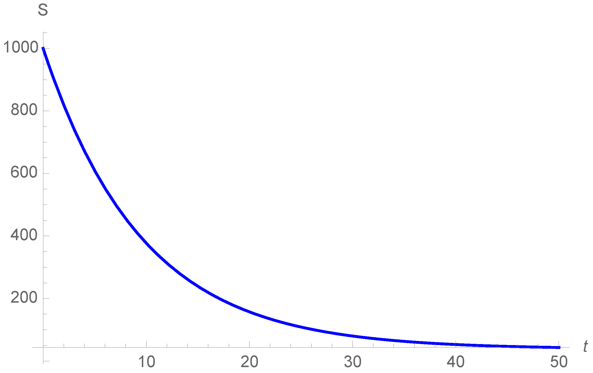
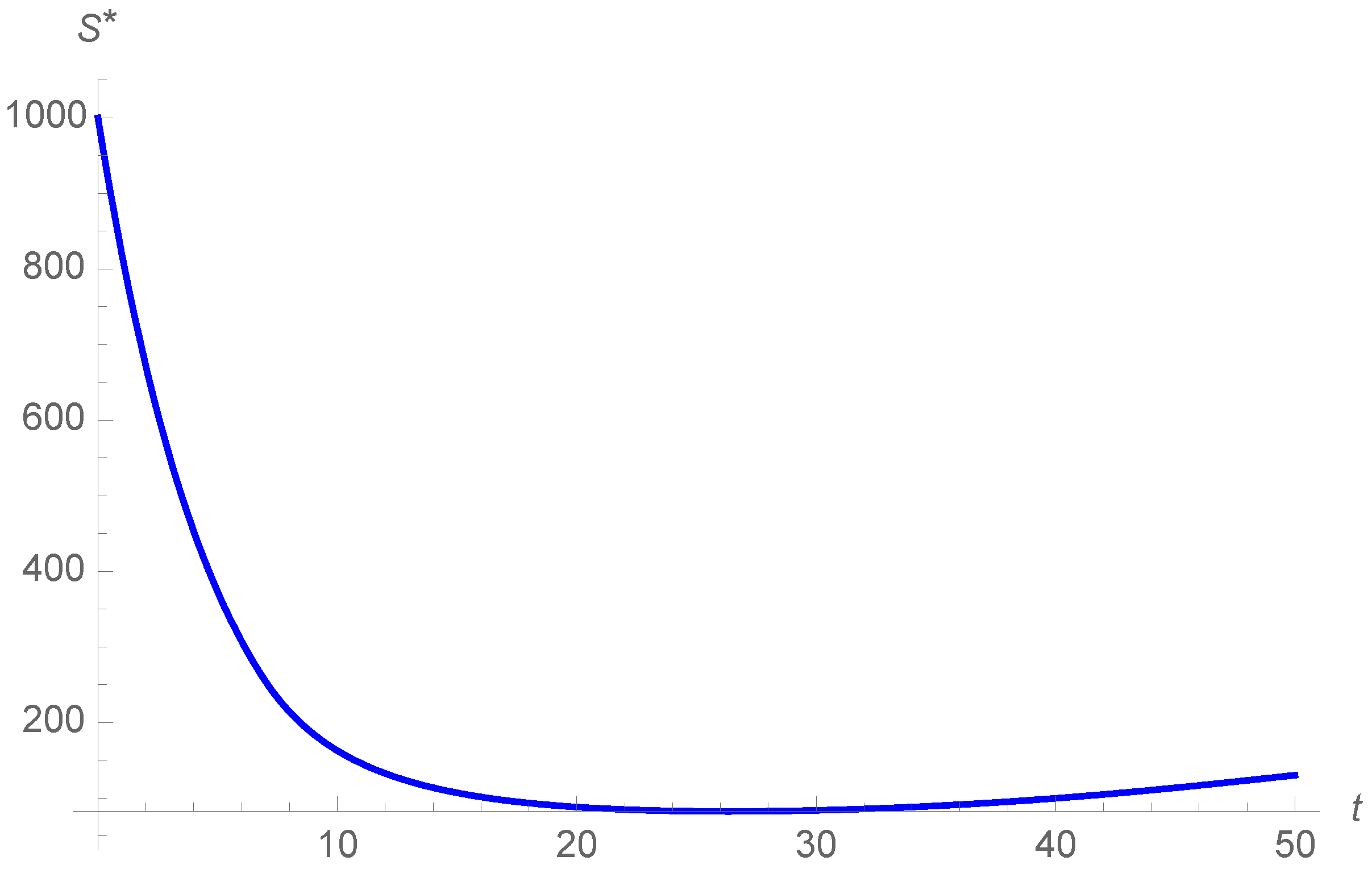
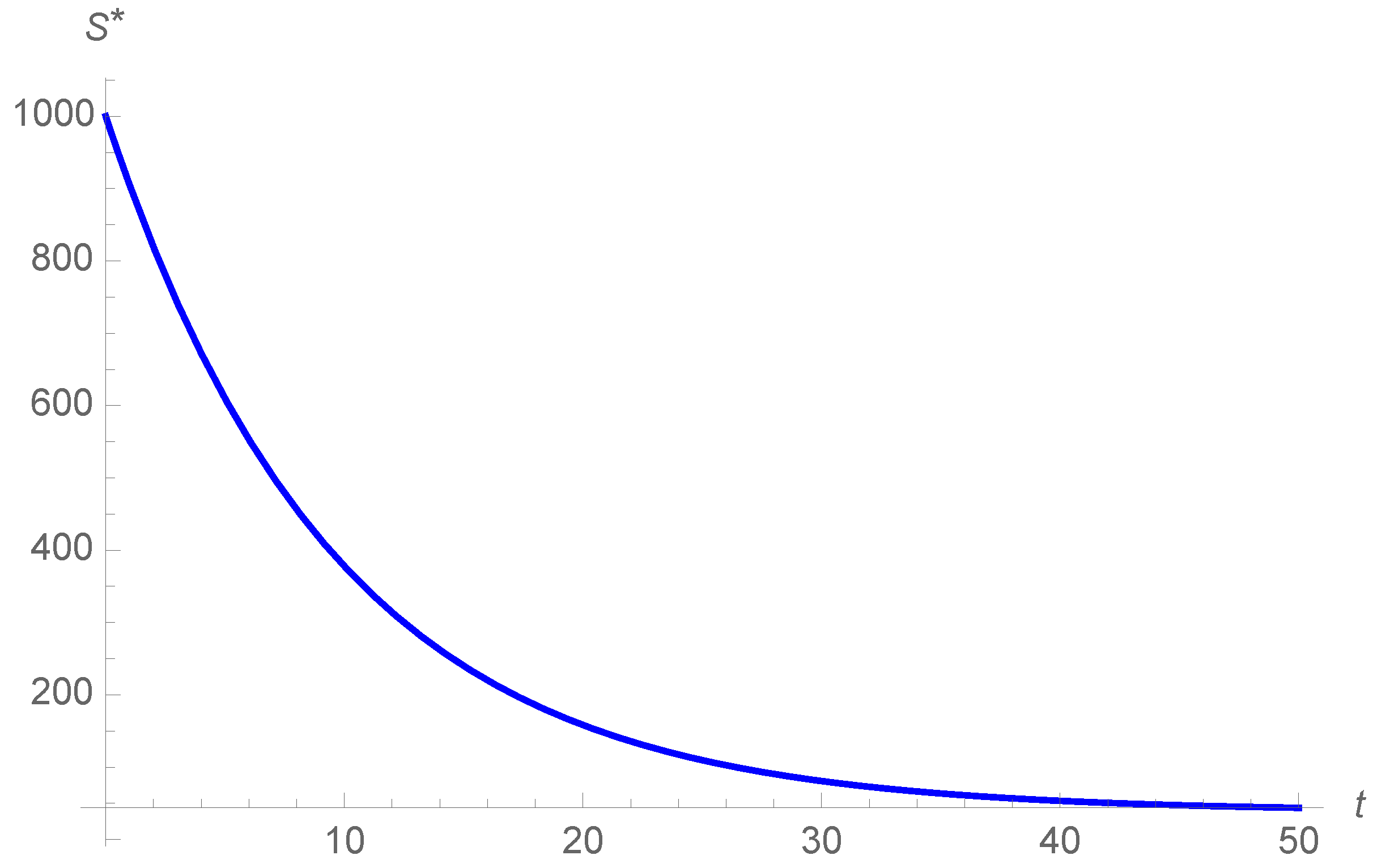
In Figure 2, Figure 3 and Figure 4, we can observe the evolution of the susceptible devices. The number of susceptible devices S decreases through time with the exception of the vaccination strategy, where the susceptible devices increase in the end. The evolution of S when considering optimal control strategies is very similar to those without control strategies.

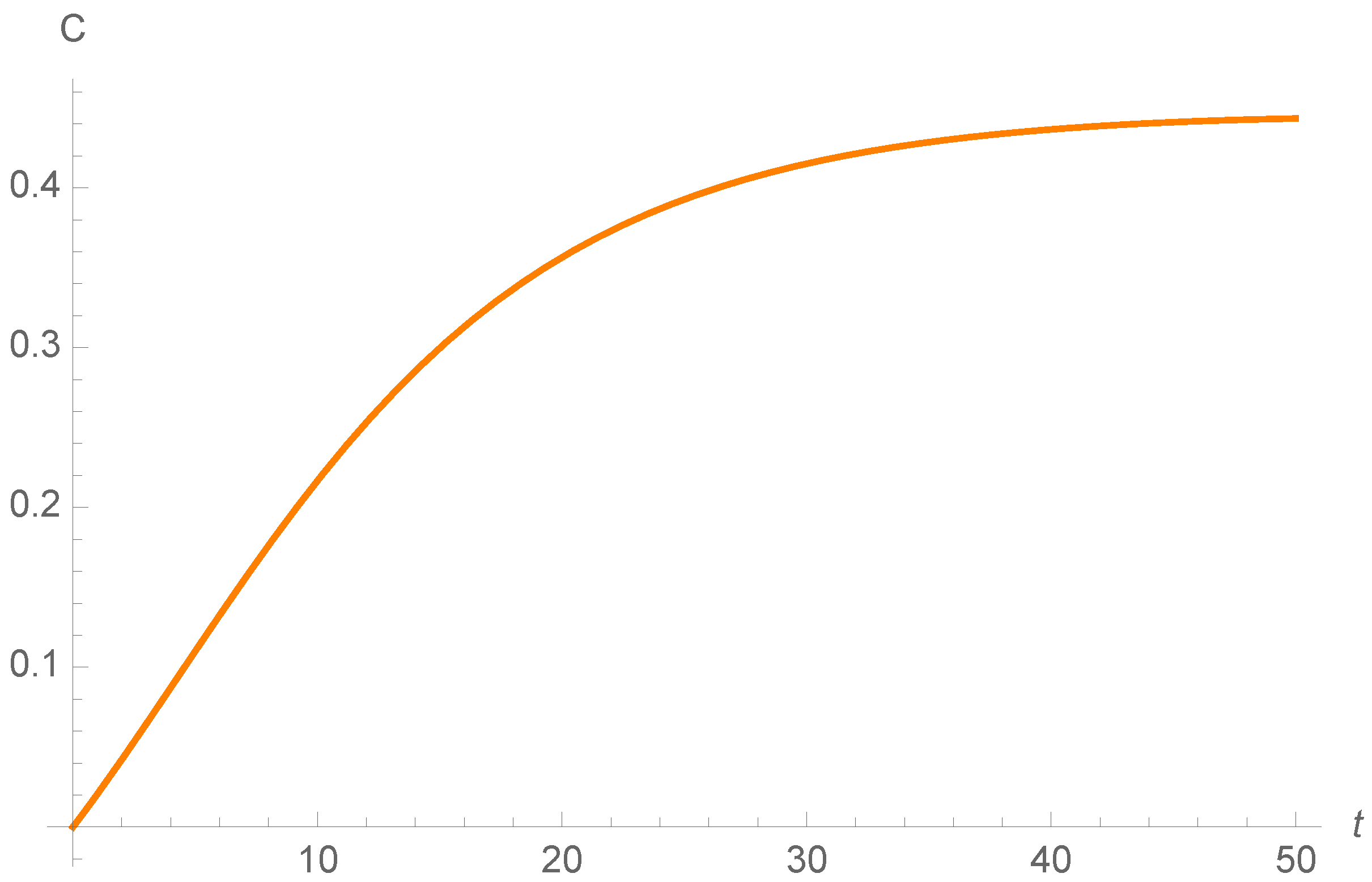
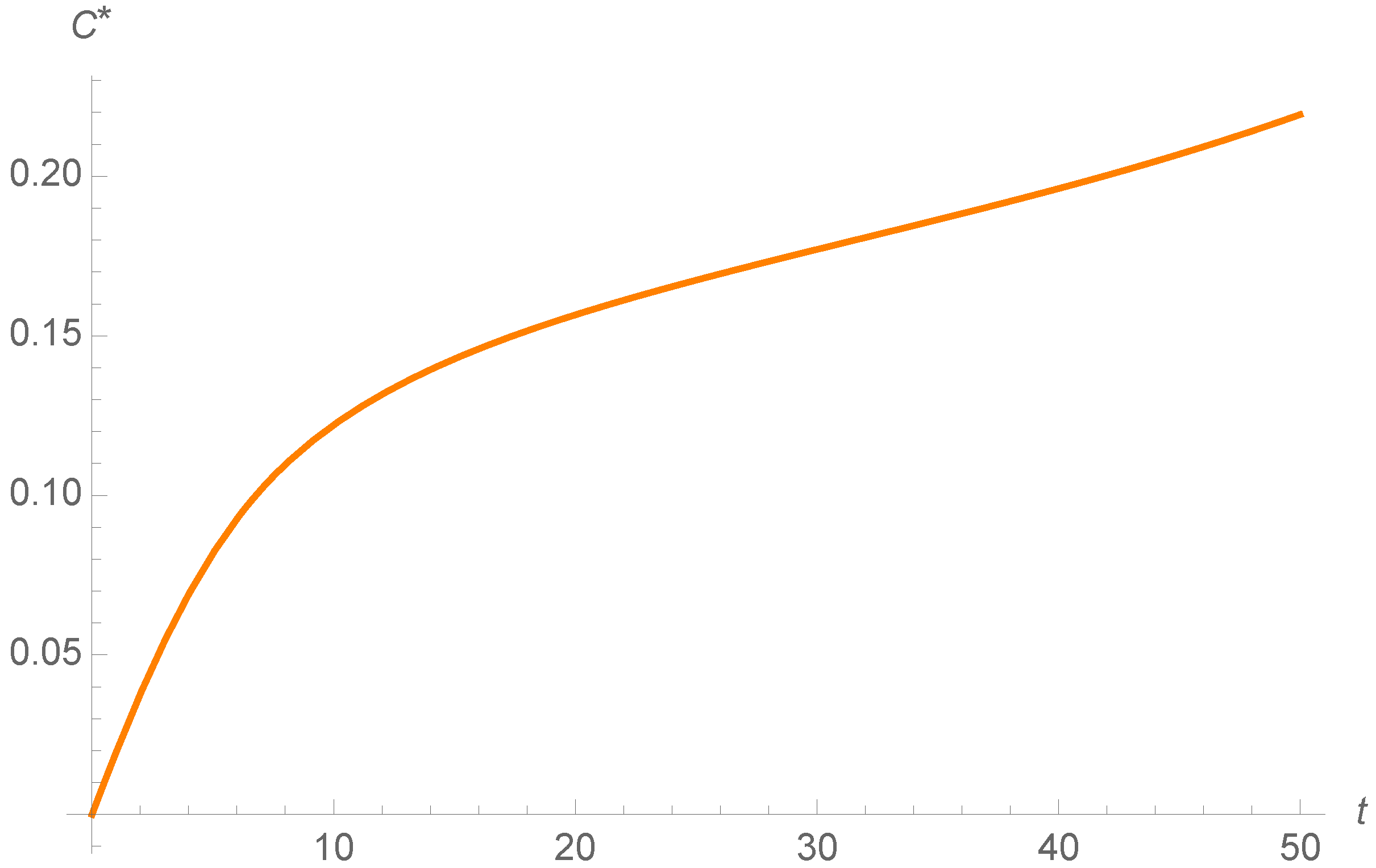
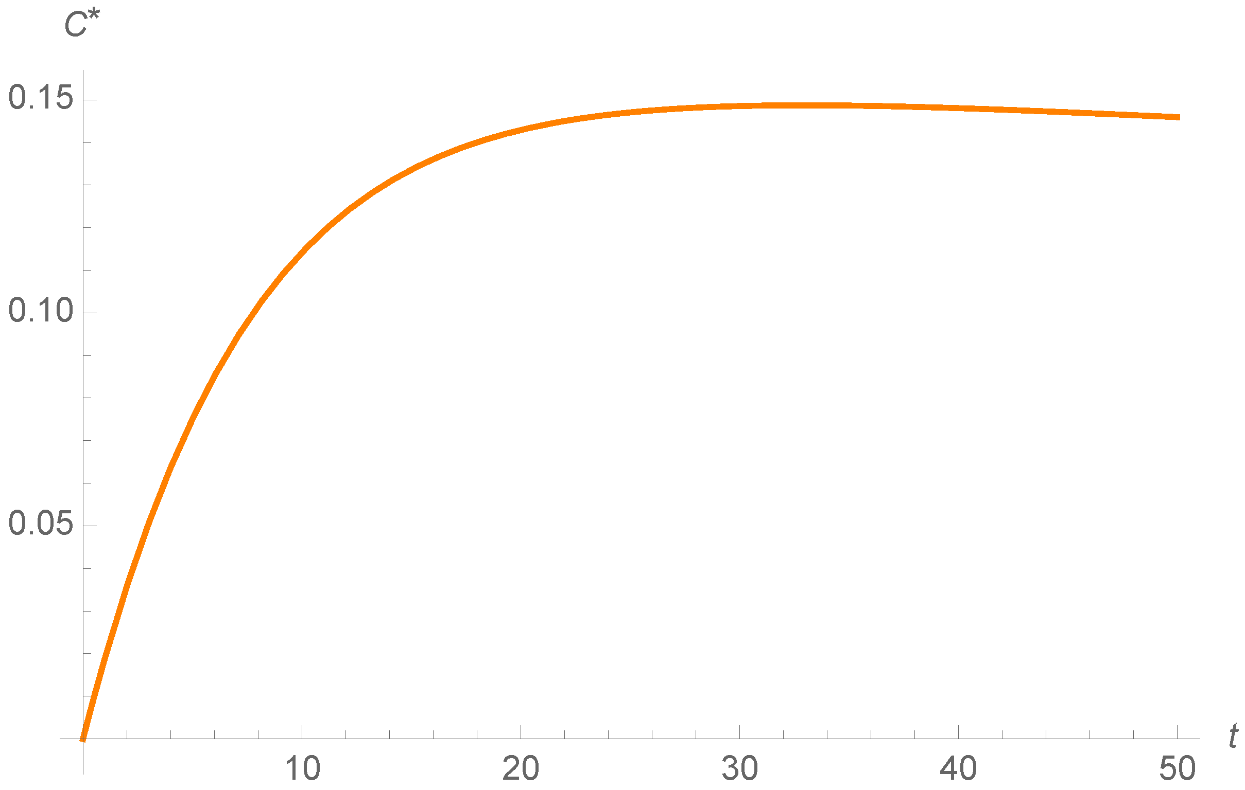
Figure 5, Figure 6 and Figure 7 show the evolution of carrier devices. When recovery strategies are considered, the graphic first increases and then decreases. However, in the case of considering vaccination strategies and no optimal control measures, the carrier devices increase a bit less than $0.5$.

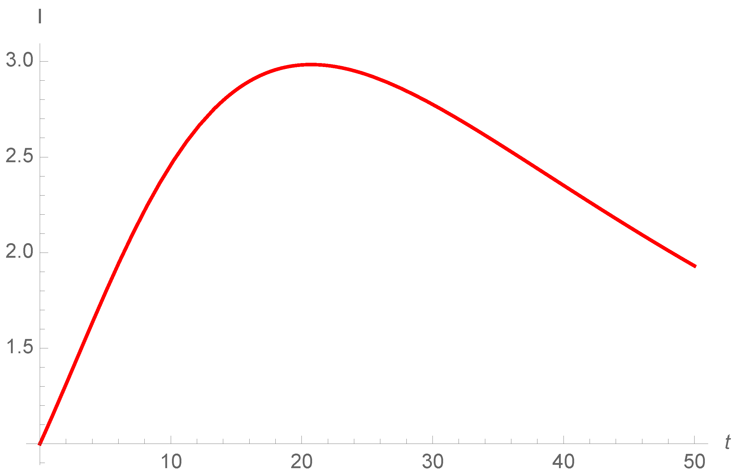
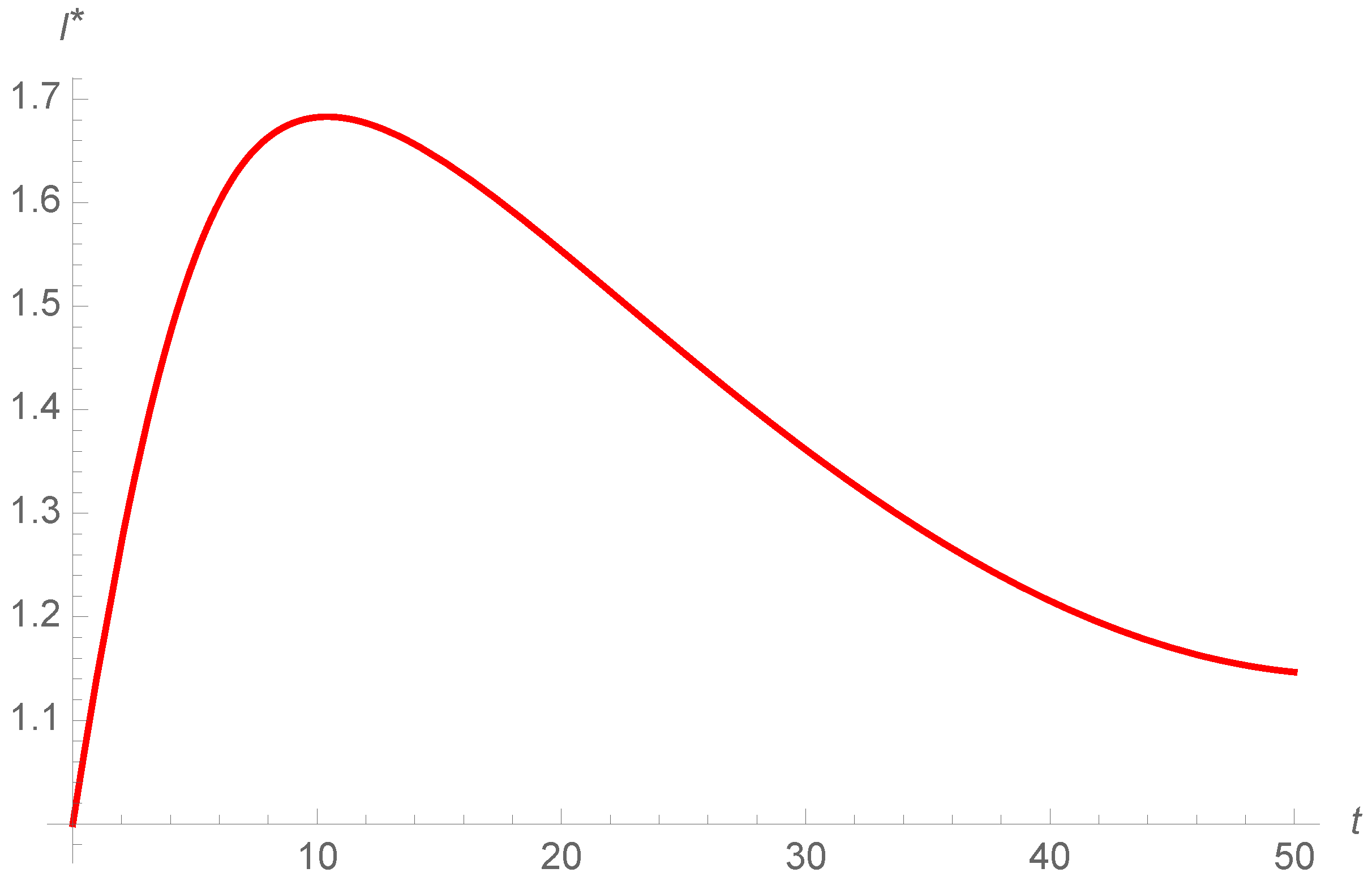
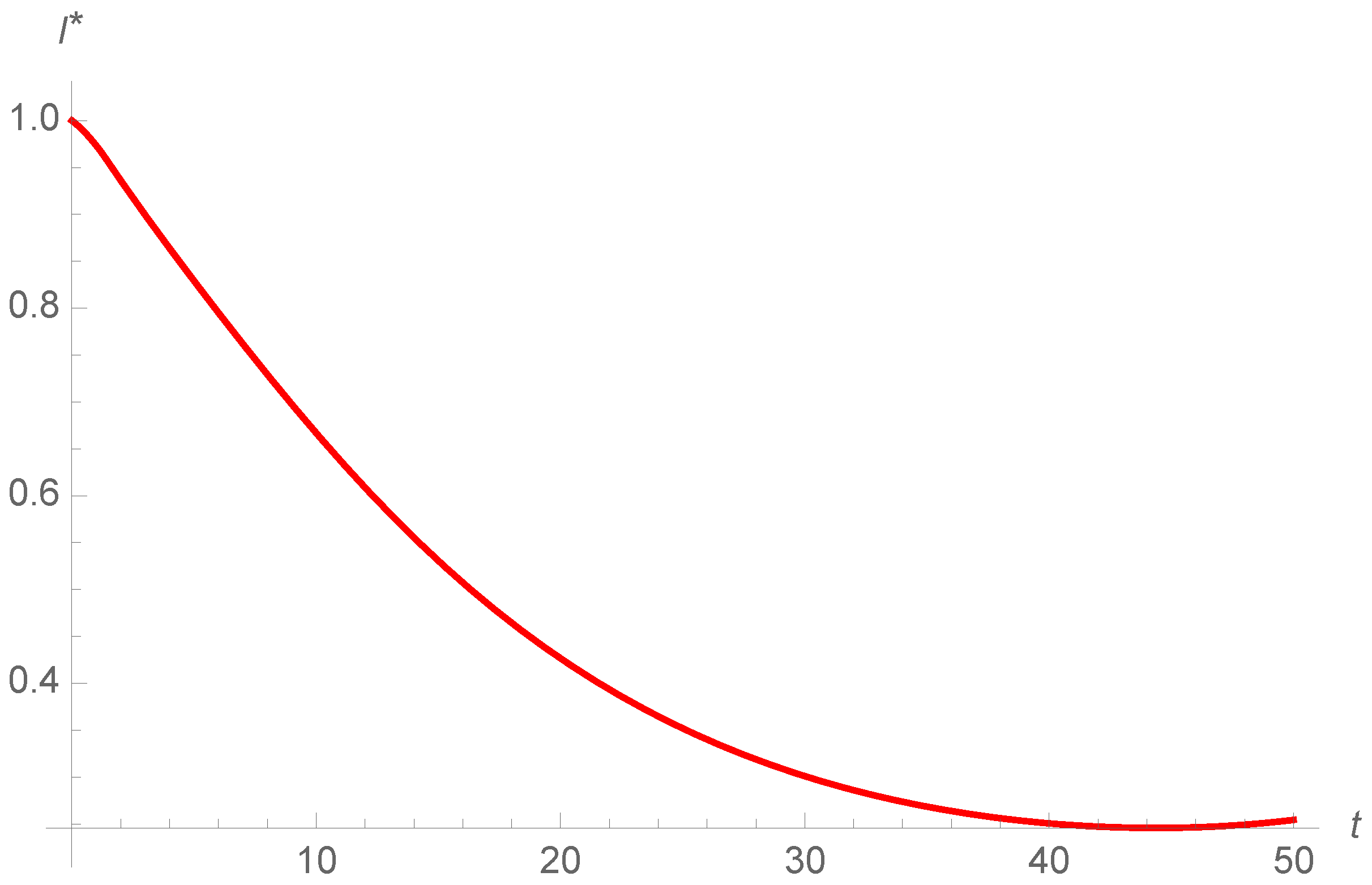
Finally, in Figure 8, Figure 9 and Figure 10, the evolution of infectious devices is shown. In both cases, with vaccination strategy and without control measures, the infectious devices increase first and then decrease. Nevertheless the infectious devices only decrease with recovery strategy. The increase is fewer than three devices. Therefore both strategies are efficient to remove the malware.

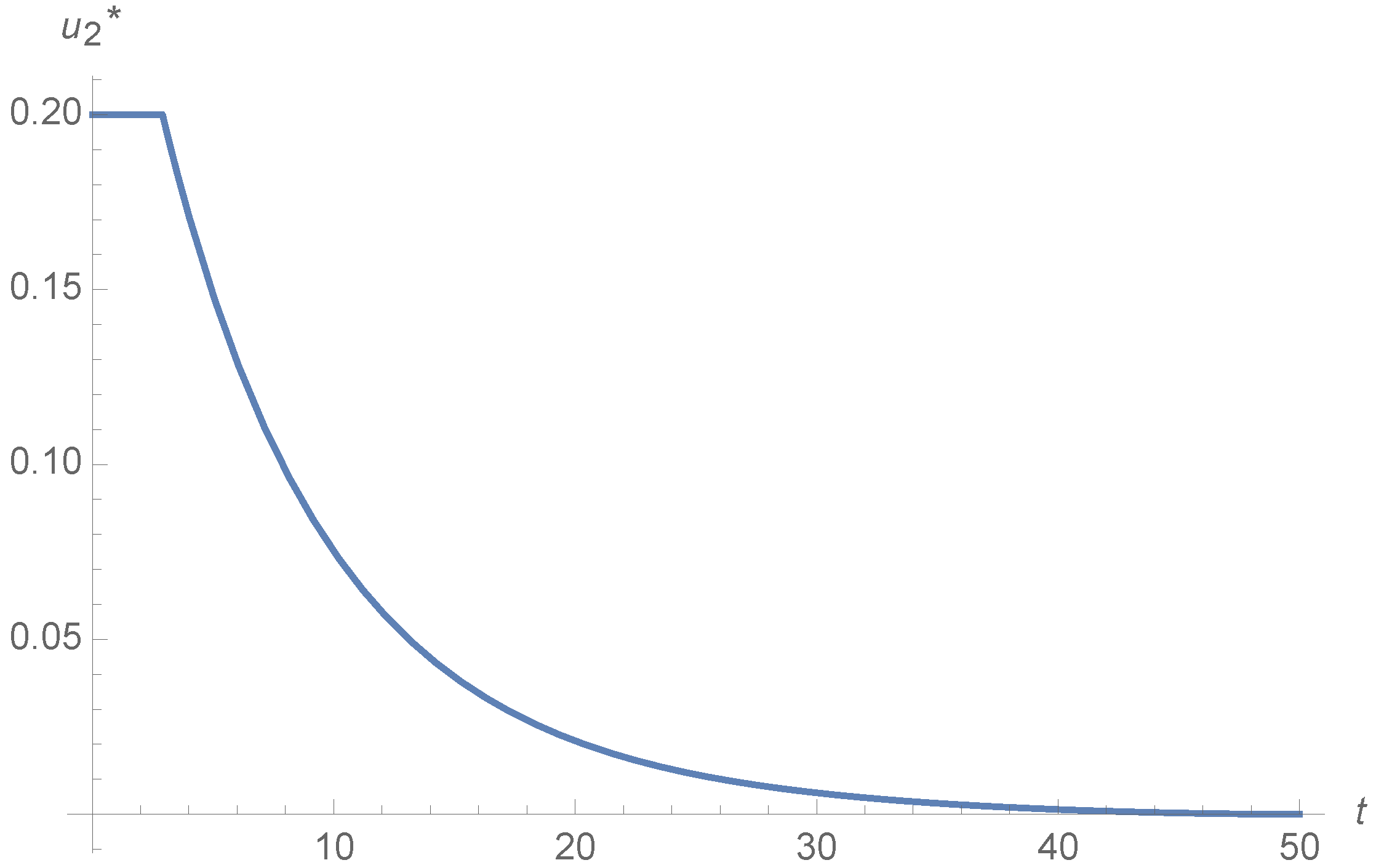
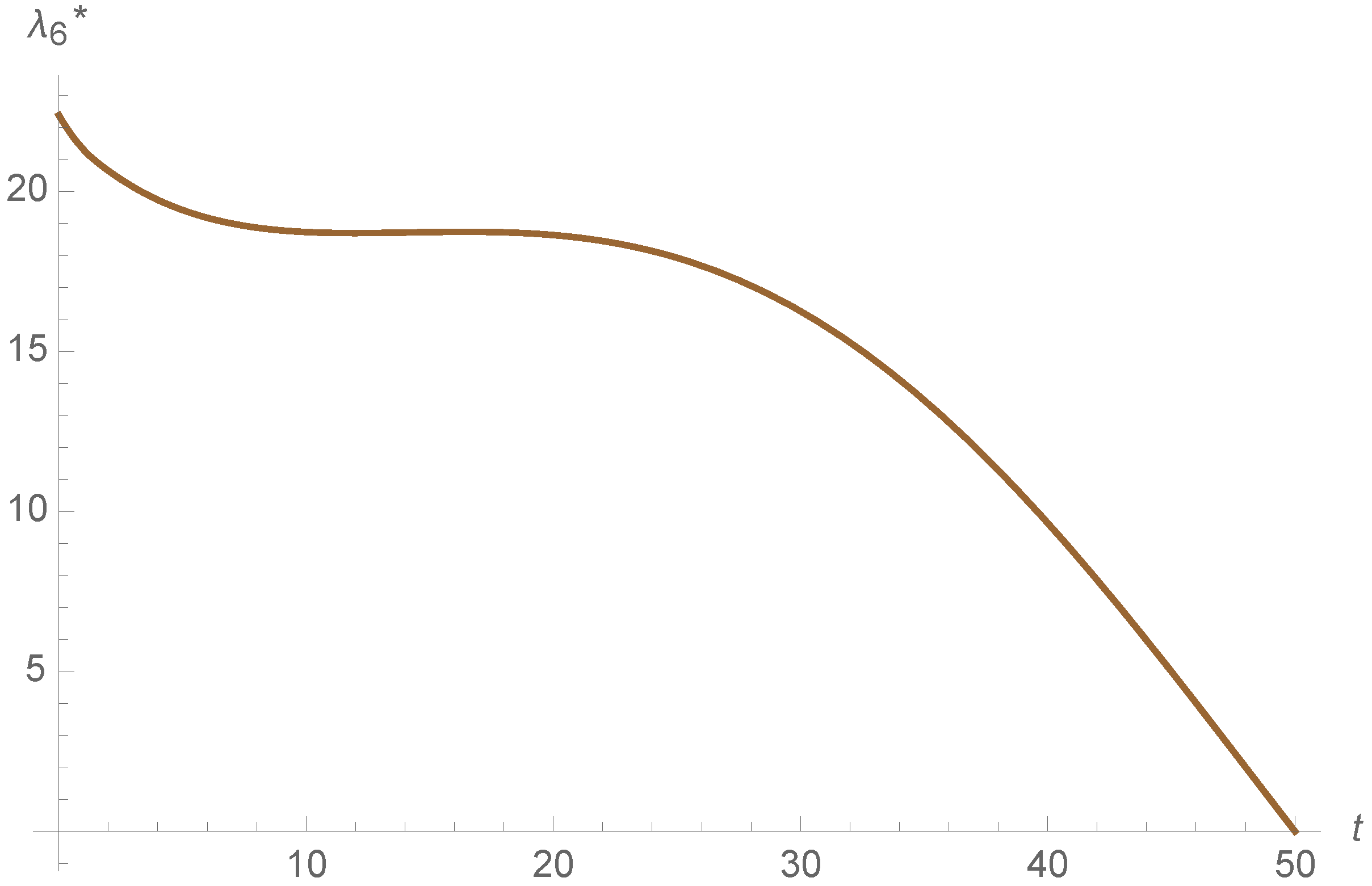
On the other hand, the evolution of the optimal control is illustrated in Figure 11 and Figure 12. We can observe how the function is constant and then it decreases considering both control strategies. This permits consider less recovery and vaccination rates through time and eliminate the epidemic. Therefore, the measures to control the epidemic are high at the beginning and we can then consider lower measures. This can help to save control measures to eliminate the epidemic without consider the same value during all the epidemic for $b_C$ or v, like taking into account prevention measures.

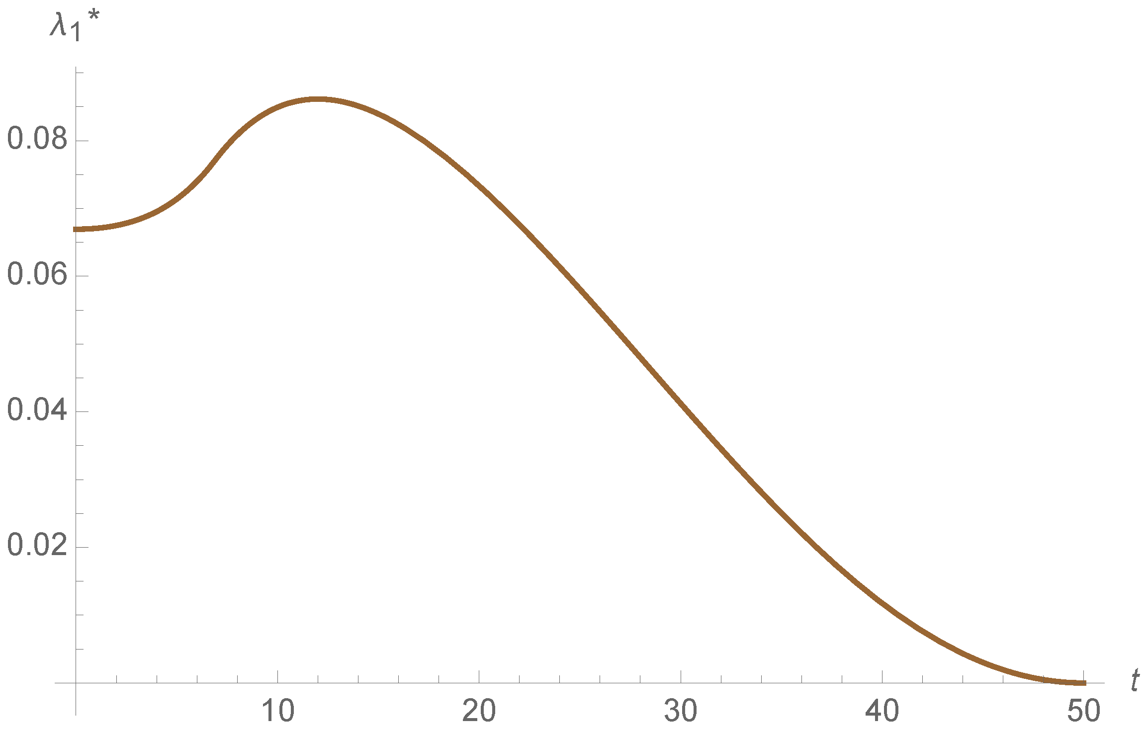
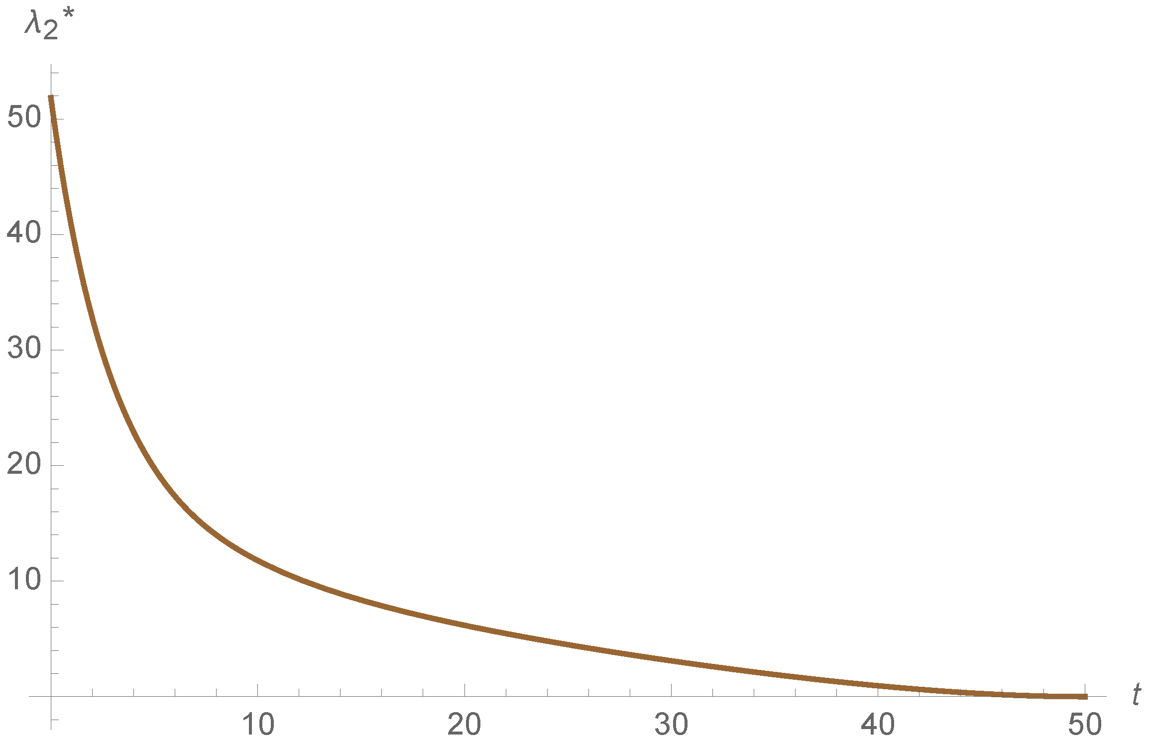
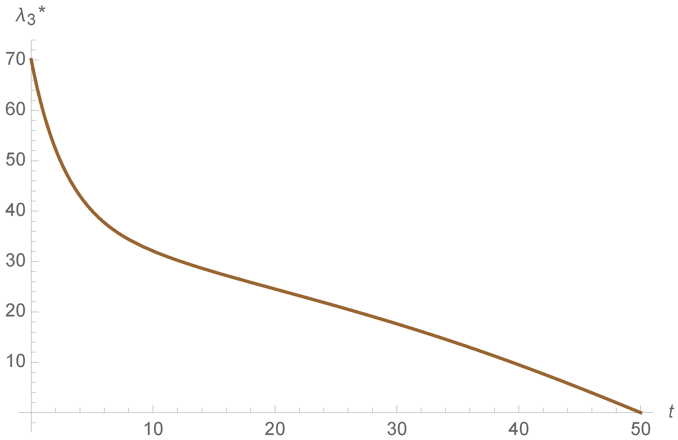
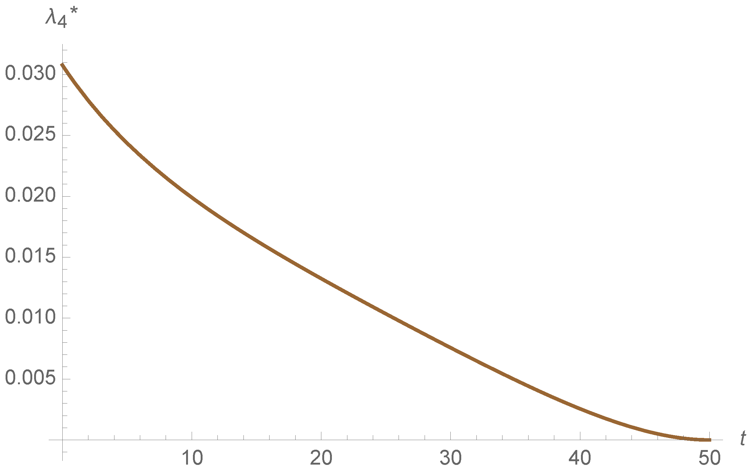
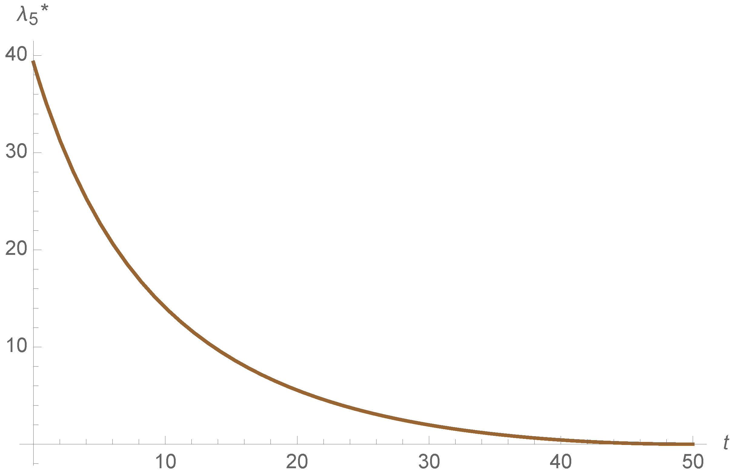
To sum up, both of the strategies are efficient in this example. However, the propagation of the adjoins functions is different in both models, as it is shown in Figure 13, Figure 14, Figure 15, Figure 16, Figure 17 and Figure 18. This indicates that the cost of the state variables is different in both control strategies. Moreover the adjoin functions satisfy the final condition ${\lambda }_i\left(T\right)=0$ for all $i=1,2,\dots ,6$, as illustrated in Figure 13, Figure 14, Figure 15, Figure 16, Figure 17 and Figure 18.

6. Conclusions

In this work, a control analysis of a model (that considers carrier devices) to simulate malware spreading is done. This permits to control the measures of recovery and vaccination; that is, we have obtained a control function that help us to decrease the number of infectious with the minimum control measures of recovery and vaccination strategies.

Note that, in this model, all of the epidemiological parameters are constant during the whole evolution. However, during the epidemic, we can apply different measures to modify some of them, while considering the control of some of this parameters. Therefore, we do not need to maintain high prevention measures in order to eliminate the malware outbreak, but we might only apply high levels at the beginning of the epidemic process. However, this kind of models are not autonomous and are more difficult to trait.

Taking into account the simulations, we can observe the behavior of the evolution of the system and the control function. Additionally, we have obtained very similar control measures with both strategies (vaccination strategy and recovery strategy). Therefore, both strategies seem to be efficient.