Using Inverse Reinforcement Learning with Real Trajectories to Get More Trustworthy Pedestrian Simulations

Abstract

Reinforcement learning is one of the most promising machine learning techniques to get intelligent behaviors for embodied agents in simulations. The output of the classic Temporal Difference family of Reinforcement Learning algorithms adopts the form of a value function expressed as a numeric table or a function approximator. The learned behavior is then derived using a greedy policy with respect to this value function. Nevertheless, sometimes the learned policy does not meet expectations, and the task of authoring is difficult and unsafe because the modification of one value or parameter in the learned value function has unpredictable consequences in the space of the policies it represents. This invalidates direct manipulation of the learned value function as a method to modify the derived behaviors. In this paper, we propose the use of Inverse Reinforcement Learning to incorporate real behavior traces in the learning process to shape the learned behaviors, thus increasing their trustworthiness (in terms of conformance to reality). To do so, we adapt the Inverse Reinforcement Learning framework to the navigation problem domain. Specifically, we use Soft Q-learning, an algorithm based on the maximum causal entropy principle, with MARL-Ped (a Reinforcement Learning-based pedestrian simulator) to include information from trajectories of real pedestrians in the process of learning how to navigate inside a virtual 3D space that represents the real environment. A comparison with the behaviors learned using a Reinforcement Learning classic algorithm (Sarsa($\lambda$)) shows that the Inverse Reinforcement Learning behaviors adjust significantly better to the real trajectories.

1. Introduction

Reinforcement learning (RL) [1] has been extensively used over the past years as a challenging and promising machine learning field in problem domains such as robot control, simulation, quality control, and logistics [2,3,4,5]. Its nature-inspired insight, based on the interaction with the environment, makes it especially suitable for solving decision-making problems in which we do not clearly know all the aspects involved in the process. RL algorithms are conceptually clear and their validity is usually demonstrated on problems that involve a discrete world with few states, a set of actions on that environment and a representation of the knowledge learned (value function) in tabular form. Nevertheless, when applying RL to real-life problems, we have to use more complex configurations based on function approximators, either linear or nonlinear ones, to represent the world states, the value function and the actions. This provides the RL model with the necessary generalization power (it can work well with states or situations never seen in the learning process), but it comes with a price tag; the representation of the learned information is hidden in the complex structure of the generalization system. Consider, for instance, that we use a neural network (NN) to approximate the value function. With this lay-out, we introduce our representation of the world as input (a vector of features or an image) and we obtain the representation of the action to take in this situation as the output. With this model, however, the learned value function can not be modified directly, if necessary, because the information is coded in the many parameters of the network, and we do not know how to map these parameters to the knowledge stored. In the simulation field, this drawback means that, in the case of the resulting learned control behavior not being suitable, we have to re-calibrate the simulator, adjust the learning elements (parameters, reward function), and begin the learning process again from scratch. That is to say, a post-processing of the learned behavior is not possible.

RL assumes that the information is in the reward function. This implies that the reward function must be adequate and precise to the task to be learned. Designing such a function with these constraints is difficult and, more importantly, is a non-methodological process. However, relatively simple reward functions have provided realistic and robust behaviors in the pedestrian simulation domain, especially in groups and crowd simulations [6,7]. In this context, the challenge arises when the designed reward does not generate realistic enough behaviors. In this case, the unique option is to re-design the reward function. Inverse Reinforcement Learning (IRL) goes a step forward in this problem, proposing a methodology for the design of the reward function based on real data provided as demonstrations of the desired behavior (see discussion of Section 2.2). IRL has two advantages with respect to RL in the simulation domain. First, IRL is actually a methodology for the automatic design of the reward function (then, the manual design of it is avoided). Second, the resulting reward is based on the information provided by real examples that guarantees that the derived behaviors conform to reality. However, the IRL approach also has drawbacks. In its classic framework, it assumes a lineal model for the reward function, which can be restrictive for some problems. Other difficulties arise in problems where a model of the environment is not available (called model-free version in the literature). In this case, the computational load is higher than RL. In fact, the model-free version includes an iterative schema with a RL process inside (see Algorithm 1).

Algorithm 1: Iterative schema for the model-free case

In this paper, we propose the use of Inverse Reinforcement Learning (IRL) to include information from the real world inside the learning process. The introduction of real examples is a way of calibrating the learning process during the process itself, guaranteeing that the learned control or the behavior is similar to that provided in the examples without giving up the power of generalization inherent to the learning process. In this work, we focus on the problem of simulating the navigation of a pedestrian inside a 3D environment representing a simple maze. We have captured real traces of pedestrian trajectories in a maze recorded in our laboratory. Then, we define an adequate IRL approach for this problem domain and compare the resulting behavior with those obtained after a classic RL process in the same domain. The results show that the IRL simulation captures fundamental aspects from the real pedestrian examples that makes the simulation more realistic than the classic RL one.

The main contribution of this paper is to adapt the IRL formalism based on maximum causal entropy to the simulation of human navigation, as a means of including data from the real world to mitigate the problem of calibrating and adjusting RL-based simulators and, thus, getting more trustworthy simulations. A challenging aspect of our problem domain is the continuous state space that implies the use of a function approximator. The importance of getting realistic pedestrian simulations is justified by the increment in the use of simulated pedestrian flows in many kinds of social and environmental simulation scenarios such as facility design, buildings and infrastructure design, crowd disasters analysis, etc. [8].

The paper is organized as follows: first, we introduce the RL and IRL fundamentals, second, we present our approach to IRL for the navigation domain, then we explain our experimental set-up and discuss the results. Finally, we present our conclusions and future work.

2. Background

In this section, we briefly introduce the fundamentals of RL and IRL.

2.1. Reinforcement Learning

RL [9] is an area of Machine Learning concerned with the problem of sequential decision-making. This problem has been modeled in decision theory as a Markov Decision Process (MDP). An MDP is a 4-tuple {$\mathcal{S}$, $\mathcal{A}$, $\mathcal{P}$, $\mathcal{R}$} where $\mathcal{S}$ is the state space, $\mathcal{A}$ is the action space, $\mathcal{P}$ defines the (stochastic) transition from one state to another, and a reward function $\mathcal{R}:\mathcal{S}\times \mathcal{A}\times \mathcal{S}\to \mathbf{R}$. The function $\mathcal{P}:\mathcal{S}\times \mathcal{A}\times \mathcal{S}\to [0,1]$ gives the probability of changing to a certain state from another one after performing an action, and models the interactions with the environment. The state signal $s_t$ describes the environment at discrete time t. Let A be a discrete set. In the state $s_t$, the decision process can select an action from the action space $a_t\in A$. The execution of the action in the environment changes the state to $s_{t+1}\in S$ following the probabilistic transition function $\mathcal{P}(s_t,a_t,s_{t+1})=Pr\{s_{t+1}=s^{\prime }\mid s_t=s,a_t=a\}$. Each decision triggers an immediate scalar reward given by the reward function $r_{t+1}=\mathcal{R}(s_t,a_t,s_{t+1})$ that represents the value of the decision taken in the state $s_t$. The goal of the process is to maximize at each time-step t the expected discounted return defined as:

$$R_t=E\left\{\sum _{j=0}^{\infty }{\gamma }^j{r}_{t+j+1}\right\}$$

(1)

where the $\gamma \in [0,1]$ parameter is the discount factor and the expectation E is taken with the probabilistic state transition $\mathcal{P}$ [10]. The discounted return takes into account not only the immediate reward got at time t but also the future rewards. The discount factor controls the importance of the future rewards. A policy is a function $\pi :S\to A$ and represents a particular behavior inside the MDP. Another way of representing a policy is as a probability distribution over the state–action pairs $\pi :S\times A\to [0,1]$. The Action-value function (Q-function) $Q^{\pi }:S\times A\to \mathbf{R}$ is the expected return of a state–action pair given the policy $\pi$:

$$\begin{array}{c}\hfill Q^{\pi }(s,a)=E\{R_t\mid s_t=s,a_t=a,\pi \}=E\{\sum _{j=0}^{\infty }{\gamma }^j{r}_{t+j+1}\mid s_t=s,a_t=a,\pi \}.\end{array}$$

(2)

The goal of the RL algorithm is to find an optimal $Q^{*}$ such as $Q^{*}(s,a)\ge Q^{\pi }(s,a)\forall s\in S,a\in A,\forall \pi$. The optimal policy ${\pi }^{*}\left(s\right)$ is automatically derived from $Q^{*}$ as it is defined in Equation (3):

$${\pi }^{*}\left(s\right)=\underset{a}{argmax}{Q}^{*}(s,a)$$

(3)

This problem is highly related with the Multi Armed Bandit problem in which it has a first motivation and benchmark [11,12,13].

Two main streams exist in the RL framework: value function algorithms and policy gradient algorithms. The former tries to find a function that maps state–action pairs with their expected return for the desired task. The latter works in the policies space trying to adjust a parametric policy via gradient ascent to find one that accomplishes the task. Soft Q-learning, used in this paper (see Section 2.2.1), should be included in the first group.

2.2. Inverse Reinforcement Learning

In RL, the source of information for the learned control or behavior is the reward function. This signal must be rich enough to evaluate all the key decisions taken in the learning process to converge to the optimal policy. Nevertheless, in many cases, the design of the reward function is difficult especially when the policy we want to find is very specific with respect to the selection of actions (i.e., a bad selection of an action can give a result far from the expected control or trajectory). In these cases, the definition of a rough reward function can be derived in unsatisfactory policies. IRL addresses the problem from another point of view. Given a set of examples taken from real life or from an expert, the goal of IRL is to find a reward function that can provide, after an RL process, a policy that generates results similar to those presented as examples [14,15,16]. Formally, given {$\mathcal{S}$, $\mathcal{A}$, $\mathcal{P}$} and a policy $\pi$ (from examples or an expert), we want to find the set of reward functions {$R_i$} where $\pi$ is an optimal policy in the MDP {$\mathcal{S}$, $\mathcal{A}$, $\mathcal{P}$, $R_i$}. In the practical cases, we are not provided with a policy $\pi$ but with a set of examples derived from it. In this case, the goal is to define rewards that generate policies consistent with the provided examples.

Several IRL approaches consider the existence of a vector $\overrightarrow{\varphi }$ of feature functions ${\varphi }_i:\mathcal{S}\times \mathcal{A}\to \mathbf{R}$ and a set of examples ${\varsigma }_i$, that is, sequences of pairs $(s_j^i,a_j^i)$ made by an expert or the real phenomena in the nature. It is assumed that the feature functions ${\varphi }_i$ measure properties that are relevant for the decision process (e.g., in the experiment proposed in [17], they are the current occupancy of a specific cell in the gridworld, in a driving simulator they can be properties of the driving style such as change of line, crash with other car...). Given an MDP, a discounted feature expectation vector is defined for a policy $\pi$ and a discount factor $\gamma$ as

$$\overrightarrow{f_{\pi }}=E\left[\sum _{t=0}^T{\gamma }^t\overrightarrow{\varphi }\right]=\sum _{t=0}^T{\gamma }^{t}E\left[\overrightarrow{\varphi }(s_t,a_t)\right]$$

(4)

In the case of the description of the real process, we do not know the implicit policy and it is estimated using the set of examples ${\varsigma }_i$

$$\overrightarrow{f_{\varsigma }}=\frac{1}{\left|\varsigma \right|}\sum _{i=1}^{\left|\varsigma \right|}\sum _{t=0}^T{\gamma }^t\overrightarrow{\varphi }(s_t^i,a_t^i)$$

(5)

These definitions are also valid for episodes with infinite time horizon ($T\to \infty$). Considering a model of the reward function as a linear combination of the feature functions $R(s,a)={\sum }_i{\theta }_i{\varphi }_i(s,a)$, the feature expectation vector of a policy $\pi$ completely determines the expected sum of discounted rewards for acting using this policy [16,17]. The goal of IRL is to optimize the reward function to generate a policy $\pi$ with a discounted feature expectation vector $\overrightarrow{f_{\pi }}$ that accomplishes:

$$\overrightarrow{f_{\pi }}=\overrightarrow{f_{\varsigma }}$$

(6)

Matching feature expectation vectors is an ill-posed problem: there are many solutions, including the degenerate solution (that is assigning probability zero to the trajectories of the set $\varsigma$) for this optimization problem. Several formulations of the IRL problem have been proposed. The work by [16] formulates the problem as a linear programming optimization while the work in [17] proposes a quadratic programming optimization problem. The difficulty with these approaches is that they provide as output a mixture of policies that guarantees in expectation Equation (6). Given a finite set of policies ${\pi }_{i}i=1,2,\dots n$, a new mixed policy can be built whose discounted feature expectation vector is a convex combination of those of the set of policies ${\sum }_{i=1}^n{\lambda }_i{\overrightarrow{f}}_{{\pi }_i}{\lambda }_i\ge 0;{\sum }_i{\lambda }_i=1$, where the probability of choosing policy ${\pi }_i$ is ${\lambda }_i$. We can calculate the probabilities ${\lambda }_i$ finding the closest point to $\overrightarrow{f_{\varsigma }}$ in the convex closure of ${\overrightarrow{f}}_{{\pi }_i}i=1,2,\dots n$ solving a quadratic programming problem [17]. In the simulation domain (and specifically in pedestrian simulation), a mixture of policies that, in expectation, satisfies feature matching is not acceptable because it can produce a feeling of random and non-realistic behaviors. Other works [18,19] have focused on avoiding the degenerate solution of the optimization problem.

Recently, the use of deep learning has been included in the IRL framework for problems with large or continuous state and action spaces. The work by [20] proposes a version of the Maximum Entropy IRL problem with a nonlinear representation of the reward function using a neural network for robotic manipulation. The work by [21] derives from the generative adversarial network paradigm a model-free imitation learning algorithm that extracts directly a policy from data.

Some of these approaches have been used in the problem domain of the pedestrian simulation. The work by [22] uses the approach discussed in [17]. The authors propose a geometric interpretation that builds a convex hull extracting critical information from the normals of the facets of that hull. The problem is that the process suffers from the curse of dimensionality with the number of chosen features. The work in [23] extends the problem to the multi-agent setting. The authors study a traffic-routing domain and find a formulation similar to that proposed in [16]. The multi-agent problem is decomposed in multiple agent-based optimizations, each one focusing on a part of the state space assuming a complete observation of it. Recently, interest has also focused on deep learning-based solutions. The work by [24] uses Deep Inverse Reinforcement Learning for multiple path planning for predicting crowd behavior in the distant future. The work by [25] implemented Inverse Reinforcement Learning using two algorithms: the Maximum Entropy algorithm and the Feature Matching algorithm to estimate the reward function of cyclists in following and overtaking interactions with pedestrians.

In this paper, we propose formulating IRL as a maximum causal entropy estimation task [26,27] to overcome the problems of policy mixture creation and degenerate solutions of the previous cited proposals. The maximum entropy principle [28] is an extensively used statement in statistics and probability theory. Applied in the IRL context, it prescribes the policy that is consistent with the example set of trajectories that has no any other assumptions (bias) about the problem or data [26]. This criterion is applied by maximizing Shannon’s expected information conditional entropy $H(\left(\overrightarrow{Y}\right|\overrightarrow{X})=E_{P(\overrightarrow{Y},\overrightarrow{X})}[-logP\left(\overrightarrow{Y}\right|\overrightarrow{X})]$, where Y are the predicted variables of the model and X are the side information about the problem that we do not want to model and the expectation is taken with respect to the joint probability of Y and X. In the MDPs context, the predicted variables $\overrightarrow{Y}$ are sequences of actions in $\mathcal{A}$ and the side information variables $\overrightarrow{X}$ are the provided sequence of states $\mathcal{S}$ generated by interaction with the environment [26]. The causal entropy [29,30] goes a step further considering that the causally conditioned probability of a random variable $A_t$ depends only on the previous sequence of states and actions occurred in the time sequence $P\left(A\right|\left|S\right)={\Pi }_{t=1}^{T}P\left(A_t\right|S_{1:t},A_{1:t-1})$ (note the double vertical line for distinguishing causal probability from conditioned probability and note that the sequences of variables go from 1 to time t and $t-1$ for states and actions, respectively. The causal entropy is then defined for an infinite horizon context as [27,31]:

$$H(A_{0:\infty }\left|\right|S_{0:\infty })=E_{P(S,A)}[\sum _{t=0}^{\infty }-{\gamma }^{t}log\pi (A_t,S_t)]=\sum _{t=0}^{\infty }{\gamma }^{t}E[-log\pi (A_t,S_t)]$$

(7)

where the expectation in each time period t is taken from the joint probability distribution of $A_t$ and $S_t$, which depends on the transition probability of the MDP ($\mathcal{P}$) and the policy $\pi$.

The formulation of IRL as a maximum causal entropy estimation is as follows:

$$\begin{array}{cc}\hfill \underset{\pi }{\mathrm{maximize}}& H\left(A_{0:\infty }\right|\left|S_{0:\infty }\right)\hfill \\ \hfill \mathrm{subject}\mathrm{to}:& \overrightarrow{f_{\pi }}=\overrightarrow{f_{\varsigma }}\hfill \\ \hfill & \pi \left(a\right|s)\ge 0\forall a\in \mathcal{A},s\in \mathcal{S}\hfill \\ \hfill & \sum _{a\in \mathcal{A}}\pi \left(a\right|s)=1\forall s\in \mathcal{S}.\hfill \end{array}$$

(8)

To solve this non-convex optimization problem, it is converted to an equivalent convex one considering a Lagrangian relaxation of Equation (8) and a dual problem formulation. From now on in this subsection, we follow the discussion and given demonstrations of [31].

First, we consider the following partial Lagrangian relaxation:

$$\begin{array}{cc}\hfill \underset{\pi }{\mathrm{maximize}}& H(A_{0:\infty }\left|\right|S_{0:\infty })+{\theta }^{\top }(\overrightarrow{f_{\varsigma }}-\overrightarrow{f_{\pi }})\hfill \\ \hfill \mathrm{subject}\mathrm{to}:& \pi \left(a\right|s)\ge 0\forall a\in \mathcal{A},s\in \mathcal{S}\hfill \\ \hfill & \sum _{a\in \mathcal{A}}\pi \left(a\right|s)=1\forall s\in \mathcal{S}.\hfill \end{array}$$

(9)

For a fixed $\theta$, the objective function can be maximized since the feasible set is closed and bounded. Then, we define $g\left(\theta \right)$ as the value of this optimization problem (Equation (9)) for a fixed $\theta$. Since any solution of the optimization problem shown in Equation (8) is feasible for this problem, this implies that $g\left(\theta \right)$ is an upper bound of the optimal value of Equation (8). The dual problem formulation finds the lowest upper bound:

$$\begin{array}{cc}\hfill \underset{\theta }{\mathrm{minimize}}& g\left(\theta \right)\hfill \end{array}$$

(10)

This is a convex optimization problem. The work by [31] proves that strong duality holds for the original problem (Equation (8)) and the dual problem (Equation (10)). Therefore, if we denote $p^{*}$ to the primal optimal value, then the following holds: $p^{*}={min}_{\theta }g\left(\theta \right)$.

We can relax the optimization problem of Equation (9) for the other constraints leading to another Lagrangian relaxation optimization problem:

$$\begin{array}{cc}\hfill \underset{\pi }{\mathrm{maximize}}& H(A_{0:\infty }\left|\right|S_{0:\infty })+{\theta }^{\top }(\overrightarrow{f_{\varsigma }}-\overrightarrow{f_{\pi }})\hfill \\ \hfill & +\sum _s{\lambda }_s(1-\sum _{a\in \mathcal{A}}\pi \left(a\right|s))\hfill \\ \hfill \mathrm{subject}\mathrm{to}:& \pi \left(a\right|s)\ge 0\forall a\in \mathcal{A},s\in \mathcal{S}\hfill \end{array}$$

(11)

Following the same reasoning than before, the dual problem

$$\begin{array}{cc}\hfill \underset{\theta ,{\lambda }_s}{\mathrm{minimize}}& g(\theta ,\lambda )\hfill \end{array}$$

(12)

is a convex optimization problem.

2.2.1. Soft Q-Learning

The practical solution of the problem formulated in Equation (12) has the form of a gradient-based algorithm [31]. It has three steps: first, find a parameterized policy ${\pi }_{{\theta }_i}$ with the current reward $R_i(s,a)={\sum }_i{\theta }_i{\varphi }_i(s,a)$. Second, evaluate the policy and calculate $\overrightarrow{f_{{\pi }_{{\theta }_i}}}$. Third, use a gradient-ascent with respect to parameters $\overrightarrow{\theta }$ to adjust the value of the linear reward. The gradient of the dual problem is $\overrightarrow{f_{\varsigma }}-\overrightarrow{f_{\pi }}$.

When the transition probabilities $\mathcal{P}$ are known, the policy can be found using Dynamic Programming. If they are not known, as in this case (model-free case), the authors propose the use of algorithm Soft Q-learning that is a variation of the Q-learning algorithm, a well-known temporal difference learning method in RL. The schema are summarized in Algorithm 1.

A Soft Q-learning algorithm uses a recursive updating rule to back-up the value function defined as:

$$Q_{t+1}(s,a)=Q_t(s,a)+\alpha (s,a)[R(s,a)+\gamma \underset{a^{\prime }\in \mathcal{A}}{\mathrm{softmax}}{Q}_t(s_{t+1},a^{\prime })-Q_t(s,a)]$$

(13)

where $\underset{a\in \mathcal{A}}{\mathrm{softmax}}Q(s,a)=log{\sum }_{a\in \mathcal{A}}\exp \left(Q(s,a)\right)$ and $R(s,a)$ is the proposed linear reward $R(s,a)={\sum }_i{\theta }_i{\varphi }_i(s,a)$. The presence of a Softmax-type distribution of the values of Q is a result of the application of the maximum entropy principle, which provides Boltzmann-like solutions. When there is a $a_i\in \mathcal{A}$ with $Q(s,a_i)$ considerably larger than the others, the update rule transforms in the Q-learning rule, selecting $\underset{a\in \mathcal{A}}{max}Q(s,a)$. On the contrary, when the values of the actions for the state s are similar, all the actions contribute in the rule.

In [31], the authors prove that this rule is a contraction that converges to a parameterized softmax policy ${\pi }_{\theta }^{\mathrm{soft}}$ that is unique. This policy is defined as

$${\pi }_{\theta }^{soft}(s,a)=\frac{exp\left(Q_{\theta }(s,a)\right)}{{\sum }_{a^{\prime }\in \mathcal{A}}\exp \left(Q_{\theta }(s,a^{\prime })\right)}$$

(14)

for a given (learned) value function $Q_{\theta }$ with fixed $\theta$.

The problem is then solved with an iterative schema where the reward is adjusted using gradient ascent to get a new policy ${\pi }_{{\theta }^{\prime }}$ by means of a Soft Q-learning process and then calculates a feature vector $\overrightarrow{f_{{\pi }^{\prime }}}$ more approximate to $\overrightarrow{f_{\varsigma }}$.

Soft Q-learning [31] is described in Algorithm 2.

Algorithm 2: Soft Q-Learning

3. IRL for the Navigation Domain

In this section, we briefly describe our problem domain and the decisions made to implement the IRL framework described in Section 2.

3.1. MDP Setup

In our set-up, an embodied 3D agent represented by a circular shape of dimensions similar to the mean personal space of a pedestrian moves inside a 3D virtual environment. The agent has a set of actions that permits to modify their speed and direction. The goal is to arrive to a target place in the environment. The state of the agent is defined in each step by a vector of real-valued features. The agent has a limited number of steps to reach the goal in one episode. At each step, the agent selects a pair of actions one for changing the speed and other to change the direction of the velocity. The environment uses a physics engine called ODE (www.ode.org) that is calibrated to represent human interaction with real environments while walking. The environment consists of two walls that configure a maze (see figures of Section 4). The embodied agent is placed in a point opposite to the goal and is tasked with reaching the target crossing the maze using the internal corridor formed by the two walls. Next, we describe briefly the main characteristics of the state space and the actions space. The interested reader can find a complete description of the environment in [6,32].

The action space is discrete and has two types of actions. One type controls the speed and the other one controls the direction of the velocity. We have divided each type of action into nine different intensities. For the type of control of the speed, these are: four to increase the speed in $\frac{1}{16},\frac{1}{8},\frac{1}{4},\frac{1}{2}$ of a reference value (maximum velocity) and four to decrease the speed in the same proportion plus a ’Do nothing’ action. For the control of the direction of velocity, we set an imaginary line between the agent and the goal. Then, we define four actions to turn to the right of the line in $\frac{\pi }{32},\frac{\pi }{16},\frac{\pi }{8},\frac{\pi }{4}$ and the same for the left of the line plus a ’Do nothing’ action.

The state space is a vector space constituted by nine real-valued features described in Table 1 and shown in Figure 1.

Table 1. State space features.

Feature	Explanation
$S_{ag}$	Speed of the embodied agent
$A_v$	Angle of the velocity respect to a line joining the agent with the goal
$D_{goal}$	Distance to the goal
$D_{o{b}_i}$	Distance to wall i
$A_{o{b}_i}$	Angle of the position of wall is relative to a line joining the agent with the goal

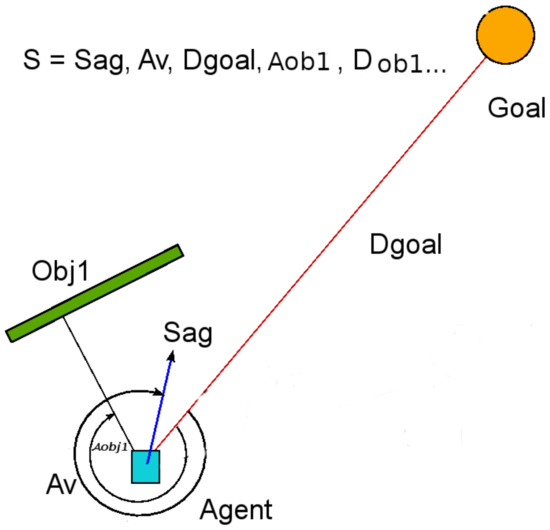
Figure 1. State space features.

Since features are continuous, this imposes the necessity of a generalization method to address the mapping of infinite values of the state space to a discrete value function $Q(s,a)$. We use a generalization method called tile coding [33] derived from CMAC [34]. It is a linear discretization function approximation method with binary sparse features. It is based on the definition of several grids that cover the state space. Each grid defines a set of cells. The representation of a point of the space is given by the active cells (those that contain the point) corresponding to each grid. The value function is then a linear combination of the active cell for a state in each time $Q(s,a)={\sum }_{i=1}^T{\omega }_i{\phi }_i$ (where T in the total number of cells of all grids, ${\phi }_i$ is a binary feature with value ’1’ if the correspondent cell i is active and ’0’ otherwise, and ${\omega }_i$ is the value of cell i that is updated by the learning algorithm. In order to face the curse of dimensionality, a hash table is used so that the cells are mapped to entries in the hash table. This method is effective when the problem is disperse, and therefore, the collisions in the same entry by different cells are rare, which is the case because the state space used by the policies in the learning process is much smaller than the whole state space. A discussion of this generalization technique in the context of RL can be found in [9].

3.2. IRL Setup

An important decision in the configuration of the IRL framework is the form of the functions ${\varphi }_i\left(s\right)$ that are used to calculate reward R and the feature expectation vectors $\overrightarrow{f_{\pi }}$ and $\overrightarrow{f_{\varsigma }}$. It is a problem domain-dependent decision. The work by [17] indicates that the functions must represent key features of the problem (e.g., the distance to an obstacle in an autonomous vehicle problem), while [31] suggests that “[the functions ${\varphi }_i(s,a)$] measure quantities that direct expert decisions”. We propose the use of radial basis functions (RBFs) based on the distance of the agent state to several prototypical states as a measure of the similarity of the learned behavior and the real trajectories. The idea is as follows: we have reproduced the real trajectories of the set of examples $\varsigma$ with an agent in our virtual 3D environment and we have collected the states through which the agent goes. Then, we have used K-means to get a set of prototypes that generalize these states. Figure 2 displays a picture of the prototypes and the data points used for the two first features of the state description. Each of these prototypes constitute the mean of a Gaussian RBF function with standard deviation $\sigma$ empirically fixed ${\varphi }_i\left(s\right)=exp(-\frac{d}{{\sigma }^2})$, where $d=\left|\right|s-p_i{\left|\right|}^2$ is the square of distance of a state s to the prototype $p_i$. Therefore, each function ${\varphi }_i\left(s\right)$ gives an estimation of the similarity of the present state s to a specific dynamic situation similar to those extracted from the real trajectories of the set of examples $\varsigma$ represented by the prototype $p_i$. Note that the state features are constituted by distances and velocities which is roughly a description of the dynamic state of the individual or agent. With this setting, the feature expectation vector $\overrightarrow{f_{\varsigma }}$ describes a behavior in terms of the distance of the states generated by the real trajectories to the prototypes. The same occurs with the expectation vector $\overrightarrow{f_{\pi }}$ with respect to the learned behavior. The gradient ascent process will adjust the reward function to get a similarity between both feature expectation vectors which also means a similarity between the dynamic situations (states) learned and those represented by the examples. The assumption under this set up is that the generation of similar dynamic situations in a task implies similar behaviors.

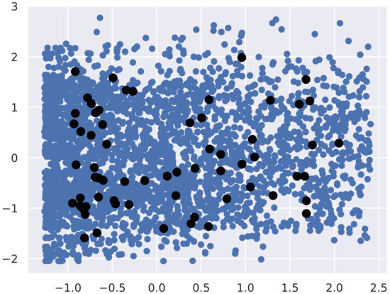
Figure 2. Prototype extraction using K-means. The set of prototypes (in black) constitutes a generalization of the observed states (in blue). The features of the states are mainly distances and velocities which represent a dynamic situation.

4. Experimental Results

The lay-out of our virtual 3D environment is shown in Figure 3 (right side). There are two walls that create a maze. The embodied agent is placed on the right of the image and the goal is to reach the place labeled with a red triangle on the left. We have carried out the same experiment in a laboratory (with the same dimensions of those in the 3D environment) with real pedestrians (See Figure 3, left side). Several trajectories have been sampled from pedestrians in the laboratory that will constitute the set of examples denominated $\varsigma$ in Section 2.2. These real sampled trajectories are shown in the 3D environment in Figure 3 (right side).

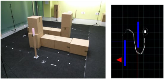
Figure 3. (Left) Real environment. The pole marks the position of the goal. The pedestrian is placed initially opposite to the pole after the farthest wall in the picture. (Right) Several sampled real trajectories displayed in the 3D environment.

As a baseline, we first try to solve the navigation problem using the standard RL setting. This problem is similar to that considered in [6] with the difference that, here, we consider only one agent inside the maze. The algorithm used is Sarsa($\lambda$) with Tile coding as the function approximator. The learning parameters are configured with the values shown in Table 2. The simplicity of the reward signal in this experiment generates undesirable trajectories that try to reach the target using the shortest path, avoiding the corridors of the maze as shown in the sequence of images in Figure 4.

Table 2. Experiment setup.

Parameter	Explanation
$\gamma =0.9$	Importance of future rewards.
$\alpha =0.002344$	Learning rate per grid of Tile coding (equivalent to 0.15)
Number of tiles = 64	Grids used in Tile coding
reward-goal = 100.0	Reward when reach the goal
Number of episodes = 20,000	Number of episodes (trials) of the learning process

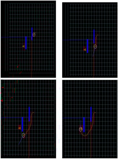
Figure 4. Sequence of images of the learned trajectory using a standard RL process with Sarsa($\lambda$) algorithm. Sarsa is a standard RL algorithm. The thick (red) line shows the learned trajectory.

Instead of designing more complex rewards to get the desired behavior, we use the examples in $\varsigma$ to setup a IRL process that learn similar paths. The parameter configuration for the IRL process is shown in Table 3. The parameters for the RL processes included inside the IRL schema are the same as Table 2. Table 4 shows the computational time for the execution of a complete schema with 100 iterations. The execution was carried out using a SGI ALTIX Ultraviolet 1000 with cores type Nehalem-EX (2.67 Ghz). Figure 5 shows the learning curve of the RL process for the final iteration of the schema described in Algorithm 1. Note that the agent carries out many episodes until the number of successful episodes increases. The agent does not reach to the goal consistently (that is, through a sequence of state–actions adequately rewarded) until about iteration 14,000. Once the $Q_{\theta }(s,a)$ values begin to converge to those that define the current policy ${\pi }_{\theta }^{\mathrm{soft}}$, the probability of using a successful state–action sequence increments. It is likely that the learning process could be finished at this point. The learned behavior after the IRL process is shown in the image sequence of Figure 6. The sequence shows that the learned behavior with the IRL framework is in accordance with the behaviors of the real pedestrian consisting of following the corridor between the walls.

Table 3. IRL experiment setup.

Parameter	Value
Number of prototypes (functions $\varphi$)	128
Number of iterations of the schema	100
Learning rate of gradient ascent $\alpha$	0.6
Number of real trajectories in $\varsigma$	3

Table 4. IRL experiment mean computation time for 10 executions (in minutes).

Parameter	Value
Time (minutes) for one iteration (one RL learning)	27.3 min
Time (minutes) for a complete schema execution (100 iterations)	2778 min

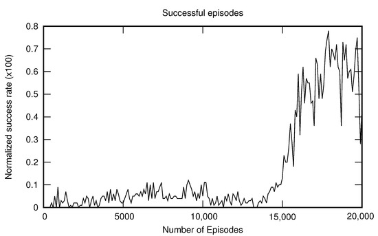
Figure 5. Learning curve for the last iteration of the schema.

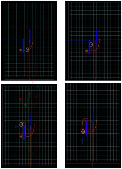
Figure 6. Sequence of images of the learned trajectory using the IRL schema. The thick (red) line is the learned trajectory.

The same experiment has been reproduced using different number of prototypes, specifically 64 and 256 prototypes. The three configurations give rational trajectories over 80% of the simulations in some of the iterations of the schema. Just because one iteration provides good results does not mean that the immediate next ones will maintain or improve them. The variations in the reward function due to the gradient ascent process creates oscillations in the learning results.

A Procrustes analysis has been carried out to determine the similarities of the shapes of the curves of the discounted feature expectation vectors $\overrightarrow{f_{\varsigma }}$ and $\overrightarrow{f_{\pi }}$. It consists of applying shape-preserving transformations to the coordinates of the curves in order to get the best fit (matching) between them. Note that the goal of the gradient ascent process described in Algorithm 1 is to minimize the difference between the feature vectors. Therefore, this similarity in shape is a measure of the quality of the optimization process. The results displayed in Figure 7 show that both curves are similar demonstrating the effectiveness of the method. The Procrustes’ distance P is the sum of the squared differences of the transformed coordinates. For the curves in our experiment, the distance is $P_{f_{\varsigma }-f_{\pi }}={10}^{-5}$. As a value reference, the Procrustes’ distance of the real feature vector $\overrightarrow{f_{\varsigma }}$ respect to a random vector with values in the same range is $P_{random}=0.0015$.

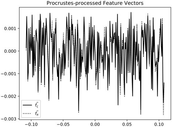
Figure 7. Curves for vectors $\overrightarrow{f_{\varsigma }}$ and the last iteration $\overrightarrow{f_{\pi }}$ after being pre-processed by Procrustes analysis. Note the similarity of both curves.

5. Conclusions and Future Work

The results of the experiment demonstrate the effectiveness of the proposed approach using the IRL framework for pedestrian navigation. In particular, the experiment empirically confirms that the vector of feature functions of Gaussian RBFs is an adequate description of the dynamics of the agent in the sense that similar vectors imply similar dynamics. Nevertheless, the proposed IRL framework is computationally expensive. We have used one hundred iterations (each one including a RL learning process) to adjust the reward to this problem. It is arguable that such computational effort is necessary for this simple case. As demonstrated in [6], a more sophisticated reward can solve this problem in the RL context. Nevertheless, the use of expert examples is an alternative in complex cases where the design of the reward is not evident. This opens the door to new ways of ’editing’ and improving behaviors obtained with RL-based simulation frameworks relying on examples provided by experts or real behaviors, as in this case. In addition, more importantly, the examples make the calibration of the learning process stronger, in the sense that the learned behaviors imitate the real ones, which improves the trustworthiness of the simulations.

Future work points towards the use of this technique in multiple-agents simulations. Moreover, a comparison with other optimization algorithms in IRL is necessary to configure an effective framework for IRL-based navigational simulations.

References

- Watkins, C.J.C.H. Learning from Delayed Rewards. Ph.D. Thesis, University of Cambridge, Cambridge, UK, 1989. [Google Scholar]
- Kober, J.; Bagnell, J.; Peters, J. Reinforcement Learning in Robotics: A Survey. Int. J. Robot. Res. 2013, 32, 1238–1274. [Google Scholar] [CrossRef]
- Waschneck, B.; Reichstaller, A.; Belzner, L.; Altenmüller, T.; Bauernhansl, T.; Knapp, A.; Kyek, A. Optimization of global production scheduling with deep reinforcement learning. Procedia CIRP 2018, 72, 1264–1269. [Google Scholar] [CrossRef]
- Gu, S.; Yang, Y. A Deep Learning Algorithm for the Max-Cut Problem Based on Pointer Network Structure with Supervised Learning and Reinforcement Learning Strategies. Mathematics 2020, 8, 298. [Google Scholar] [CrossRef]
- Novak, D.; Verber, D.; Dugonik, J.; Fister, I. A Comparison of Evolutionary and Tree-Based Approaches for Game Feature Validation in Real-Time Strategy Games with a Novel Metric. Mathematics 2020, 8, 688. [Google Scholar] [CrossRef]
- Martinez-Gil, F.; Lozano, M.; Fernández, F. MARL-Ped: A multi-agent reinforcement learning based framework to simulate pedestrian groups. Simul. Model. Pract. Theory 2014, 47, 259–275. [Google Scholar] [CrossRef]
- Martinez-Gil, F.; Lozano, M.; Fernández, F. Emergent behaviors and scalability for multi-agent reinforcement learning-based pedestrian models. Simul. Model. Pract. Theory 2017, 74, 117–133. [Google Scholar] [CrossRef]
- Helbing, D.; Brockmann, D.; Chadefaux, T.; Donnay, K.; Blanke, U.; Woolley-Meza, O.; Moussaid, M.; Johansson, A.; Krause, J.; Schutte, S.; et al. Saving Human Lives: What Complexity Science and Information Systems can Contribute. J. Stat. Phys. 2015, 158, 735–781. [Google Scholar] [CrossRef] [PubMed]
- Sutton, R.S.; Barto, A.G. Reinforcement Learning: An Introduction, 2nd ed.; The MIT Press: Cambridge, MA, USA, 2018. [Google Scholar]
- Kaelbling, L.P.; Littman, M.L.; Moore, A.W. Reinforcement Learning: A Survey. Int. J. Artif. Intell. Res. 1996, 4, 237–285. [Google Scholar] [CrossRef]
- Auer, P.; Fischer, P. Finite-time analysis of the multiarmed bandit problem. Mach. Learn. 2002, 47, 235–256. [Google Scholar] [CrossRef]
- Bertsekas, D.; Tsitsiklis, J. Neuro-Dynamic Programming, 1st ed.; Athena Scientific: Belmont, MA, USA, 1996. [Google Scholar]
- Niño-Mora, J. Computing a classic index for finite-horizon bandits. INFORMS J. Comput. 2011, 23, 254–267. [Google Scholar] [CrossRef]
- Kalman, R.E. When Is a Linear Control System Optimal? J. Basic Eng. 1964, 86, 51–60. [Google Scholar] [CrossRef]
- Boyd, S.; Ghaoui, E.E.; Feron, E.; Balakrishnan, V. Linear Matrix Inequalities in System and Control Theory; SIAM: Philadelphia, PA, USA, 1994. [Google Scholar]
- Ng, A.; Russell, S. Apprenticeship learning via inverse reinforcement learning. In Proceedings of the 17th International Conference on Machine Learning, Stanford, CA, USA, 29 June–2 July 2000; pp. 663–670. [Google Scholar]
- Abbeel, P.; Ng, A.Y. Apprenticeship Learning via Inverse Reinforcement Learning. In Proceedings of the Twenty-First, International Conference on Machine Learning (ICML’04), Banff, AB, Canada, 4–8 July 2004. [Google Scholar]
- Ramachandran, D.; Amir, E. Bayesian inverse reinforcement learning. In Proceedings of the Twentieth International Joint Conference on Artificial Intelligence (IJCAI’07), San Francisco, CA, USA, 6–12 January 2007; pp. 2586–2591. [Google Scholar]
- Neu, G.; Szepesvári, C. Apprenticeship learning using inverse reinforcement learning and gradient methods. In Proceedings of the Twenty-Third Conference on Uncertainty in Artificial Intelligence (UAI’07), Vancouver, BC, Canada, 19–22 July 2007; pp. 295–302. [Google Scholar]
- Finn, C.; Levine, S.; Abbeel, P. Guided Cost Learning: Deep Inverse Optimal Control via Policy Optimization. In Proceedings of the 33rd International Conference on International Conference on Machine Learning (ICML’16), New York, NY, USA, 19–24 June 2016; Volume 48, pp. 49–58. [Google Scholar]
- Ho, J.; Ermon, S. Generative Adversarial Imitation Learning. In Proceedings of the 30th International Conference on Neural Information Processing Systems (NIPS’16), Barcelona, Spain, 5–10 December 2016; pp. 4572–4580. [Google Scholar]
- Lee, S.J.; Popovic, Z. Learning Behavior Styles with Inverse Reinforcement Learning. ACM Trans. Graph. 2010, 29, 1–7. [Google Scholar]
- Natarajan, S.; Kunapuli, G.; Judah, K.; Tadepalli, P.; Kersting, K.; Shavlik, J. Multi-Agent Inverse Reinforcement Learning. In Proceedings of the Ninth International Conference on Machine Learning and Applications, Washington, DC, USA, 12–14 December 2010; pp. 395–400. [Google Scholar]
- Fernando, T.; Denman, S.; Sridharan, S.; Fookes, C. Neighbourhood context embeddings in deep inverse reinforcement learning for predicting pedestrian motion over long time horizons. In Proceedings of the 2019 International Conference on Computer Vision Workshop (ICCVW 2019), Seoul, Korea, 27 October–2 November 2019. [Google Scholar]
- Alsaleh, R.; Sayed, T. Modeling pedestrian-cyclist interactions in shared space using inverse reinforcement learning. Trans. Res. Part F Traffic Psychol. Behav. 2020, 70, 37–57. [Google Scholar] [CrossRef]
- Ziebart, B.; Bagnell, J.A.; Dey, A.K. Modeling interaction via the principle of maximum causal entropy. In Proceedings of the 27th International Conference on Machine Learning (ICML’10), Haifa, Israel, 21–24 June 2010; pp. 1255–1262. [Google Scholar]
- Ziebart, B.; Bagnell, J.A.; Dey, A.K. The principle of maximum causal entropy for estimating interacting processes. IEEE Trans. Inf. Theory 2013, 59, 1966–1980. [Google Scholar] [CrossRef]
- Jaynes, E.T. Information theory and statistical mechanics I and II. Phys. Rev. 1957, 106, 620. [Google Scholar] [CrossRef]
- Kramer, G. Directed Information for Channels with Feedback. Ph.D. Thesis, Swiss Federal Institute of Technology (ETH), Zurich, Switzerland, 1998. [Google Scholar]
- Permuter, H.H.; Kim, Y.H.; Weissman, T. On directed information and gambling. In Proceedings of the IEEE International Symposium on Information Theory, Toronto, ON, Canada, 6–11 July 2008; pp. 1403–1407. [Google Scholar]
- Zhou, Z.; Bloem, M.; Bambos, N. Infinite time horizon maximum causal entropy inverse reinforcement learning. IEEE Trans. Autom. Control 2018, 63, 2787–2802. [Google Scholar] [CrossRef]
- Martinez-Gil, F.; Lozano, M.; Fernández, F. Calibrating a Motion Model Based on Reinforcement Learning for Pedestrian Simulation. In Proceedings of the 5th International Conference on Motion in Games (MIG’12), Rennes, France, 15–17 November 2012; pp. 302–315. [Google Scholar]
- Sutton, R. Generalization in Reinforcement Learning: Successful examples using sparse coarse coding. Adv. Neural Inform. Process. Syst. 1996, 8, 1038–1044. [Google Scholar]
- Albus, J.S. A New Approach to Manipulator Control: the Cerebellar Model Articulation Controller (CMAC). J. Dyn. Syst. Meas. Control 1975, 97, 220–227. [Google Scholar] [CrossRef]
Sample Availability: Samples of the experimental data and trajectories of the embodied agents are available from the authors. Code available upon request to the authors. |
© 2020 by the authors. Licensee MDPI, Basel, Switzerland. This article is an open access article distributed under the terms and conditions of the Creative Commons Attribution (CC BY) license (http://creativecommons.org/licenses/by/4.0/).