Abstract
This research presents the epileptic focus region localization during epileptic seizures by applying different signal processing and ensemble machine learning techniques in intracranial recordings of electroencephalogram (EEG). Multi-scale Principal Component Analysis (MSPCA) is used for denoising EEG signals and the autoregressive (AR) algorithm will extract useful features from the EEG signal. The performances of the ensemble machine learning methods are measured with accuracy, F-measure, and the area under the receiver operating characteristic (ROC) curve (AUC). EEG-based focus area localization with the proposed methods reaches 98.9% accuracy using the Rotation Forest classifier. Therefore, our results suggest that ensemble machine learning methods can be applied to differentiate the EEG signals from epileptogenic brain areas and signals recorded from non-epileptogenic brain regions with high accuracy.
1. Introduction
Epilepsy is a neurological disorder where abnormal or asynchronous neuronal activity of the brain, known as the symptoms of seizures, are present [1,2]. Electroencephalogram (EEG) signals represent a crucial approach for evaluation of epileptic behavior [3]. One of the key issues for neurosurgery is the detection of early seizure discharge which helps in defining the brain area as the source of abnormal activity [3].
EEG signals acquired from the brain support our understanding of how the brain functions [4,5]. One of the aims of EEG recordings is to detect the brain areas where seizures begin and to estimate if the subject’s condition could be improved by neurosurgical removal of problematic brain areas.
Therefore, the localization of epileptic foci represents a very important stage for surgical treatment planning by detecting the earliest time of seizure onset in electroencephalographic (EEG) recordings. Epileptic foci are characterized as the region(s) in the brain which may be removed by surgical treatment to achieve control of epileptic seizures. Therefore, two different sets of signals were used. Focal EEG signals are taken from brain zones where the ictal EEG signal is detected, whereas non-focal EEG signals are taken from brain zones not involved at seizure onset [6].
The start of the ictal activity is defined by spike clusters which originate at the most active brain zones. Detection of this active brain area defined by these spike clusters can lead to precise detection of epileptogenic foci in the surgical assessment [7]. Ochi et al. [8] proposed the analysis of long interictal EEG signals to discover as many spike clusters as possible which share similar morphology and topography. Furthermore, the spike number in a cluster is compared to the total spike number to estimate its influence on the overall interictal activity. Nevertheless, this visual investigation takes time, and hence, an automated detection algorithm is needed. Wilson et al. [9] proposed a technique for spike activity recognition according to its topography and morphology. Consequently, a more accurate estimation of the group of events present in EEG recordings was achieved [7].
In our previous studies, the authors presented the approach of choosing the optimal feature extraction technique for classification of non-focal and focal EEG signals. The results showed that the time-consuming Wavelet Packet Decomposition (WPD) feature extraction algorithm together with the Random Forest algorithm achieved an accuracy of 99.92%. In this study, the idea is to use a simpler feature extraction algorithm coupled with ensemble machine learning algorithms [6].
Unwanted noise has an impact on the quality of all biosignals, including the EEG. There are two types of noise: physiological and technical noise. Heartbeat, eye, or muscle movement generate physiological noise. Apart from these, technical noise is generated by light radiation, environmental power-line interference, and medical instrumentation emitting radio frequencies. On the other hand, the EEG signals are also mixed with wideband noise and complex stochastic processes; therefore, their interpretation is challenging. Moreover, the EEG signals recorded from different patients are heterogeneous. Therefore, removing noise is a significant difficulty in biomedical signal processing analysis and applications [10,11,12]. In this research, EEG signals are preprocessed using the Multi-scale Principal Component Analysis (MSPCA) to decrease the noise.
Converting the original set of features/attributes into a smaller set of features/attributes is called feature selection. It prevents the redundancy in high-dimensional data [13]. In this research, autoregressive (AR) methods were applied for feature extraction in order to analyze discharges of epileptiform in EEG signals in the frequency domain.
Ensemble machine learning techniques are algorithms that combine the outputs of multiple learners to achieve better performance. Therefore, much less complex learners can be combined to reach great performance. Furthermore, ensembles are inherently parallel algorithms, and are much more efficient during training if exposed to multiple processors [14].
In this study, intracranial EEG signals taken from patients with pharmaco-resistant focal-onset epilepsy were utilized. The purpose of these signals was to detect the brain region to be surgically removed in every epileptic patient. This led to usage of two kinds of signals. Focal signals are acquired from the brain region where the variations of ictal EEG signals were observed. On the other hand, non-focal signals are acquired from brain regions not involved at the seizure’s onset [15]. Moreover, EEG signals are preprocessed using the MSPCA to decrease the noise. The autoregressive (AR) Burg algorithm is responsible for feature extraction from the time to frequency domain. Ensemble machine learning methods are being fed with these features to recognize the changes in each segment of the brain during the onset of a seizure. The localization of epileptic regions was then compared to real brain locations defined by the medical neurosurgeons [16].
Section 2 covers the introduction of the EEG dataset and algorithms used for signal processing (MSPCA and AR Burg). In this section, we also cover machine learning tools: Artificial Neural Network (ANN), k-nearest neighbors (k-NN), Support Vector Machine (SVM), C4.5, Reduced-error pruning tree (REP Tree), Alternating Decision Tree (AD Tree), Logical Analysis of Data (LAD Tree), Random Forest (RF) and Classification And Regression Trees (CART) and introduce ensemble machine learning techniques (Bagging, Boosting, AdaBoost, MultiBoost, Random Subspace Method, and Rotation Forest). Section 3 presents the results using total accuracy, F-measure, and receiver operating characteristic (ROC) area. Discussion and concluding remarks follow in Section 4 and Section 5, respectively.
2. Materials and Methods
2.1. Dataset
In this study, intracranial EEG signals from five epilepsy patients are used and publicly available [6]. Satisfactory surgical results were obtained from all five patients. Three patients achieved total recovery from epileptic seizures, and the remaining two subjects had auras only, but did not require additional surgery. EEG signals were acquired by using invasive electrodes and were filtered from 0.5 to 150 Hz. EEG signals were sampled at 1 GHz and then down-sampled to 512 Hz. All channels in which the changes in the ictal EEG were observed were defined as “focal EEG channels”. At least two neurologists and board-certified electroencephalographers observed the changes using visual inspection. “Non-focal EEG channels” involved the rest of the channels that were not classified as focal channels. After the analysis of EEG signals from five epileptic patients, the dataset consisted of 1000 focal EEG signals and 1000 non-focal EEG signals [15].
2.2. Multiscale Principal Component Analysis (MSPCA)
Let us consider the input signal matrix , where n is the number of measurements (samples) and m is the number of signals. Principal Component Analysis (PCA) converts this input matrix into two new matrices, L and S, such that the following holds:
where L represents the matrix of principal component loadings, and S is the matrix of principal component scores. Each column of L contains coefficients for one principal component. The columns are in descending order in terms of principal component variances, i.e., the eigenvalues, λi, of the covariance matrix of X. Matrix S is the representation of X in the principal component space. The eigenvalues define how much variance the related principal component accounts for. They can show how many variables are truly important so that the dataset can be reduced. The contribution of principal components whose eigenvalues are close to zero is usually negligible and they can be excluded [10,11,12,13,17].
The continuous wavelet transform (CWT), ω(s,τ), of a continuous-time signal, x(t), is defined by comparing the signal, x(t), to the probing function, ψs,τ(t):
creating two-dimensional mapping onto the time-scale domain.
The discrete wavelet transform (DWT) usually accomplishes the coefficient frugality by limiting the variation in scale and sliding to powers of 2. If the selected wavelet belongs to an orthogonal family, the DWT even represents a non-redundant bilateral transform.
Dyadic sampling of the two wavelet parameters is defined as,
where j and k are both integers. Therefore, the discretized probing function becomes:
s = 2−j, τ = k2−j
ψj,k (t) = 2j/2ψ(2jt − k)
Inserting Equation (4) into Equation (2), the discrete wavelet transform (DWT) is derived:
The original signal is recovered by the inverse DWT, or the wavelet series expansion
where ψj,k(t) is a set of orthonormal basis functions [18].
Multiscale PCA (MSPCA) uses the capability of PCA to eliminate the variables’ cross-correlation. The signals are decomposed by wavelet transform to combine the strengths of PCA and wavelets. This results in data matrix X transform into a data matrix WX, where WX is an n x m orthonormal matrix as a result of the orthonormal wavelet transform. The stochastic behavior in each signal is almost decorrelated in WX, but the deterministic behavior in every signal in X is preserved in a quite small number of coefficients in WX. Since the quantity of principal components to be reserved at each scale does not change the fundamental relationship between the variables at any scale, it is not transformed by the wavelet decomposition [10,11,19].
2.3. AR Burg Algorithms
The model-based techniques can be used for spectrum estimation of a dataset. One of the most frequently applied parametric techniques are AR methods, where estimation of AR parameters is constructed around the minimization of the forward and backward prediction error. AR Burg calculates the constraints of a filter. The parameters can be considered as Finite Impulse Response (FIR) predictor parameters, hence the power spectrum may be considered. In the AR Burg method, data (x(n), 0 ≤ n ≤ N−1) can be modeled as output of an all-pole, discrete, and causal filter, with a white noise input. Then, the AR Burg technique of order p can be represented as:
where AR coefficients are and is white noise [20].
Different issues must be taken into consideration, like the optimum estimation technique selection, model order selection, the signal length which will be modeled, and the stationary data level, to achieve a stable and high-performance AR technique [20,21,22,23,24].
The AR Burg method was applied to generate the power spectral density (PSD) of de-noised EEG signals. PSD values were used as inputs to machine learning techniques.
2.4. Machine Learning Methods—Single Classifiers
Artificial Neural Networks (ANN) is the machine learning model that tries to solve problems in the same way as the human brain does. Instead of neurons, ANN is using artificial neurons, also known as perceptron. In the human brain, neurons relate to axons, while in the ANN, weighted matrices are used for connections between artificial neurons. Information travels through neurons using connections between them; from one neuron, the information travels to all neurons connected to it. Adjusting the weights between a neurons system can be trained from input examples [25]. The artificial neural network is organized into multiple layers, where each layer contains multiple neurons. The information inside of the network travels from input layers to the output layers. Between input and output layers, the artificial neural network can have zero or more hidden layers. The number of layers and number of neurons inside the artificial neural network is called the architecture of the neural network [25]. In the artificial neural network, the smallest building block is the perceptron that has multiple weighted inputs, bias input, and the activation function. Propagating signal from input to the output in the artificial neural network is called forward propagation, while propagating signal from output to input is called back propagation. The most popular algorithm for training artificial neural networks is called the backpropagation algorithm [26].
The types of artificial neural networks depend on architecture, neuron activation function, loops in architecture, learning algorithm, and other attributes. Also, there are types of artificial neural networks that are capable of learning without human interaction.
Backpropagation is the most used algorithm for training artificial neural networks. This algorithm is based on an optimization method called gradient descent. In a nutshell, the algorithm has three phases: forward propagation, error calculation, and weights’ updates. When the input data sample is propagated through the artificial neural network, then the output is calculated. The output of the input sample is compared with expected output and the error is calculated. The error is used to do backward propagation and update weights in all layers to make the error minimal. This process has been repeated for every data sample from input. This process is repeated until artificial neural network mean square error reaches the desirable level [26].
k-Nearest Neighbor (k-NN): In the machine learning area, the k-NN algorithm is one of the oldest classifications and regression algorithms. The algorithm uses very simple logic to determine the output of the system based on K-nearest neighbors for input from feature space. This algorithm belongs to the category of lazy learning algorithms because the computation is postponed as much as possible. This means that the input dataset is not processed to build the model, but the model performs all computation during testing time [27,28].
The input data into the k-NN algorithm contains feature vectors and a label that represents the category of that vector. During classification, the input to the model is number k, that represents several neighbors to refer to for classification and the unlabeled input vector. The k-NN model will produce output based on k-nearest neighbors and the major label from those k neighbors will be the output label for the input vector. As explained before, the main attribute of the k-NN algorithm is the distance metric for input vectors. The most commonly used metric is the Euclidean distance. For variables from the discrete set, such as text and voice, the Hamming distance is used. For problems from biology such as microarray, different metrics can be used, such as the Pearson metric or the Spearman metric. There are implementations of the k-NN algorithm that use more advanced metrics such as NCA (Neighbor Component Analysis) and LMN (Large Margin Neighbor) [23].
The main problem of the k-NN machine learning algorithm is that major voting based on k nearest neighbors is problematic in cases when we have skewed categories. This causes the most frequent categories to dominate over those that are less frequent, leading towards a big classification error for this type of algorithm [23]. To overcome this issue inside the metric, function weights are introduced. The closer neighbors have more impact on classification than those which are farther. The output label is determined by multiplying weight with the inverse of neighbors’ distance.
The machine learning area has other algorithms that are trying to overcome this issue, like self-organized maps. To determine the best number for the parameter k, it is necessary to know some heuristics about input data. The general rule is that larger values of the k result in better classification accuracy, but boundaries between classes are not distinct. There are methods based on meta heuristics like hyper-parameter optimization that could be used to choose number k for the k-NN algorithm. Mainly, performance of the algorithm is dependent on the input data and it is very common that input data is pre-processed by some feature scaling, noise reduction, or a similar method before k-NN classification. When choosing number k, it is desirable that that number be an odd number so majority voting cannot be a draw. Evolutionary algorithms are often used to pre-process input data and to determine number k [29]. In case of high redundancy in the input vector space, feature extraction is usually applied to remove unnecessary noise. The input vector space is transformed into reduced new input space. The most used methods for feature extraction are the Haar method, mean shift tracking analysis, Principal Component Analysis, Fisher Linear Discriminant Analysis (LDA), and others [29].
Support Vector Machines: A classifier from the category of the supervised machine learning algorithms is Support Vector Machines (SVM), also known as Support Vector Networks. SVM can be used for solving classification and regression problems. For an input dataset, SVM can make a binary decision and decide in which, between the two categories, input 46 sample belongs. The SVM algorithm is trained to label input data into two categories that are divided by the widest area possible between categories. Because of this wide area between category labels, SVM is also known as a large margin classifier. The SVM model is the linear classifier and it cannot map nonlinear functions without the usage of the kernel [25].
The classification of data is the most common problem in the machine learning algorithms. The SVM algorithm represents input data samples as vectors in the n-dimensional space and the algorithm builds a linear formula for a hyper plane in (n−1)-dimensional space that separates labels between planes. There is an infinite number of hyperplanes that can separate labels in space but the SVM algorithm is designed to choose the hyperplane that has the maximum distance between both labels’ categories [30,31]. Vapnik [32] recommended that the hyperplane method, f(x) ∈ F, be selected in a functions group with enough capability. Actually, F covers functions for linearly separable hyperplanes using the next universal approximator as:
Every training example, xi, is given a weight, wi, and the hyperplane is a weighted combination of whole training samples [25].
Assume that the clear meaning of the nonlinear function, ϕ(·), has been avoided by the kernel function usage, determined properly as the nonlinear function’s dot products
and the Equation (8) transforms into
This technique is generally attributed to Mercer’s theorem [30]. The classifier which is trained then has the following form:
Decision Tree (DT) Algorithms: Nodes in a decision tree test the importance of a feature. The node test sometimes compares the value of a feature to a constant. In other cases, two features can be compared to each other, or a function is applied to features. A new sample is classified by routing it down the tree regarding the feature values established in consecutive nodes. Once a leaf has been reached, the sample is classified according to the class associated to the leaf [33]. Reduced-error pruning tree (REPTree) is an algorithm which is created by using information growth and it is reduced by reduced-error pruning. Speed optimization is achieved by sorting values for numeric features and utilizing missing values in the same way as C4.5 [31]. The alternating decision tree (ADTree) is applied for two-class issues and creates a decision tree modified by boosting [31]. LogitBoost ADTree (LADTree) is an alternative decision tree algorithm which is applied for problems with multiple classes in the LogitBoost algorithm. The iterations number is a parameter which defines the scope of the tree generated, like ADTree [31]. The classification and regression tree (CART) applies the minimum cost-complexity strategy for pruning. For instance, every test may be a linear attribute value combination for numeric attributes. Hence, the output tree represents a hierarchy of linear models [31].
Random Forest: Breiman [34,35] presented a random forest classifier which contains many classification trees. Every tree could be a classifier and the outputs of classification from all trees define the general classification output. Moreover, this general output of classification is completed by selecting the mode of all tree outputs for classification. The phases for the structure of the random forests (RF) may be concluded as follows:
- The learning process of the RF classifier starts with the construction of each tree.
- Generating the training dataset for every tree.
- This training set is named the in-bag dataset, and it is made using the bootstrapping method. The training dataset epoch number and the epoch number in the in-bag dataset are the same. In the in-bag set, around 30% of the data is repeated, so the rest of training dataset, named as out-of-bag, is applied to check the performance of tree classification. Different bootstrap samples construct each tree.
- For every tree, to build the random tree classifier nodes and leaves, we have to select and use a random number of features. If we look at Breiman [35], the casual collection of features raises the classification correctness, reduces the data noise sensitivity, and reduces the features’ correlation [36].
- At the last step, the tree including all the training datasets starts to construct a random tree.
The leading phase includes selecting a characteristic at the root node and after that, dividing the training data into subsets. This creates a division for every potential characteristic value. The splitting and the range of the root node are completely in order of information gain of the characteristic dividing. The information gain (IG) of separating the training dataset (Y) into subsets (Yi) may be defined as follows:
The operator |·| is the scope of the set and E(Yi) is the entropy statistic [37] of the set Yi, defined as:
where N is the sleep stages number to be classified (N = 5) and pj is the sleep stage proportion j in the set (Yi). If the information gain is positive, the node is divided. If it is negative, the node stays the same and becomes a leaf node that is assigned a class label. The quality collection is done according to the highest information gain of the residual qualities. The splitting procedure stays until qualities are chosen. The classification output is the most happening (active) stage of sleep in the subset for extending training nodes [36].
2.5. Ensemble Machine Learning Methods
Random Tree Classifier is defined as an algorithm which is ensemble learning and generates a couple of individual learners. Every node is divided by means of the best division between all features in a standard tree [31,38].
Bagging: A combination of different methods’ decisions results in joining the different results into a single decision. When we talk about classification, the easiest way to implement this is voting, but, if we are dealing with prediction of numeric values, it is calculation of the average.
Specific decision trees could be present as experts. Trees could be combined by voting on every test case. One class is taken as correct if it receives more votes than others. Predictions which are the results of voting are more consistent if we take more votes. If we include new datasets for training, it unusually makes worse decisions, it builds trees for them, and predictions of these trees contribute in the vote. Bagging tries to remove the instability of learning techniques by way of simulating a method defined before applying a certain training set. The original training data is modified by removing some samples and duplicating the others instead of sampling a new training dataset each time. Random sample is applied on instances from the original dataset with replacement to generate a new dataset. This sampling process necessarily removes some of the instances and replicates the others. Bagging only resamples the native training data instead of generating autonomous datasets from the domain. The datasets obtained by resampling vary from each other but are definitely not independent because one dataset is the base for all of them. Nevertheless, it seems that bagging generates a combined model that usually performs better than the single model made from the native training data and is never significantly worse. There is one difference, where the individual predictions are averaged, which is a real number instead of voting on the result [31].
The boosting is a technique for involving multiple models by searching for models that complement each other. Boosting employs voting or averaging to combine the result of each model, like bagging [31].
AdaBoost may be used in any learning algorithm, similar to bagging. Any learning algorithm can handle weighted instances, which is a positive number. The weights of instance are used to calculate the classifier’s error. By doing so, the learning algorithm will concentrate on a particular set of instances with high weight. The AdaBoost algorithm starts by assigning the same weight to all training data instances and then by forcing the learning method to create a classifier for this data and reweights every instance according to the output of the classifier [31].
MultiBoosting: Bagging and AdaBoost seem to work with dissimilar mechanisms, and we can combine these two methods by obtaining the benefits of them. Actually, bagging generally decreases variance, while AdaBoost decreases both bias and variance. Furthermore, bagging achieves more of an effect than AdaBoost at decreasing [39] variance and their combination can hold AdaBoost’s bias reduction while increasing bagging’s variance reduction. Since bagging minimizes the number of examples for training available to form each sub-committee, we can use wagging [39] to eliminate this drawback. As a result, MultiBoosting can be defined as wagging committees formed by AdaBoost. In order to set the number of sub-committees, MultiBoosting uses a single committee size argument and then it defines a target final sub-committee member index by setting an index for each member of the final committee, starting from one. Moreover, MultiBoosting has the power computational advantage over AdaBoost in which the sub-committees can be learned in parallel, while this would necessitate an adjustment in the functioning of premature learning in a sub-committee termination. Since the AdaBoost is intrinsically sequential, it reduces the potential for parallelization. On the other hand, every classifier learned with wagging is not depending on others, which allows parallelization, a gain that MultiBoosting gets at the sub-committee level [40].
Rotation Forest: The classification accuracy can usually be improved by considering the grouping of a few classifiers—a procedure known as classifier ensemble. Rotation Forest represents a technique for constructing classifier ensembles based on the process of feature extraction. Initially, the set of feature vectors is arbitrarily divided into K subsets and PCA is carried out to each subset. The variability in the data is preserved by keeping all principal components. Consequently, the new features for a basis classifier are formed by means of rotations of the K axis. The rotation takes care of supporting variety within the ensemble via feature extraction for every basis classifier. The term “forest” is used as Decision Trees (DTs) were selected as base classifiers due to their sensitivity to rotation. The preservation of all principal components will take care of individual accuracy. In addition, accuracy is pursued as the whole dataset is used for training every base classifier. Rotation Forest ensembles are able to form more accurate and diverse individual classifiers than the ones using AdaBoost, Random Forest, and Bagging approaches [41].
The Random Subspace Method (RSM) is a combination of methods introduced in Reference [42]. The training data is also modified in the RSM by changing the feature space in such a way that it gains the r-dimensional subspace, which is random of the original p-dimensional space of the feature. Hence, the transformed training set contains r-dimensional training objects. As a result, one may create classifiers in the random subspaces. Therefore, the last decision rule combines them via majority vote. The RSM can be beneficial for applying random subspaces for creating and aggregating the classifiers. If the training objects’ number is not big compared to the size of the data, one can resolve the small sample size issue by creating classifiers in random subspaces. The original feature space is bigger than the dimensionality of subspace, though the training objects’ number keeps the same value [43].
3. Results
In this research, EEG signals are recorded from patients with epilepsy in order to determine the focal area of the epileptic seizures. Focus region localization has been investigated at the epileptic seizure by the application of machine learning methods to identify the seizure activity onset. After the analysis of EEG signals from 5 epileptic patients, the dataset consisted of 1000 focal EEG signals and 1000 non-focal EEG signals. Firstly, EEG recordings were pre-processed using Multi-Scale PCA in order to decrease the noise level. Later, the autoregressive Burg method was applied for extraction of features.
The results have been produced on a PC with the Intel Core i7-4710HQ 2.5 GHz central processing unit (CPU), 16 GB of RAM, and 256 GB of solid-state drive (SSD) storage. All the machine learning algorithms have been implemented in Java programming language using Waikato Environment for Knowledge Analysis (WEKA) [44]. Due to the lower number of publicly available samples in the dataset (2000 EEG signals), 10-fold cross-validation was used to evaluate the performance of machine learning algorithms. The performances of the machine learning methods were measured with accuracy, F-measure, and the area under the Receiver Operating Characteristic (ROC) curve. Accuracy values will show to what extent our analysis compares with what medical neurosurgeons had found in their patients.
Table 1 and Table 2 present the performance for different evaluation criteria used in this paper for ten machine learning techniques which are used in combination with single classifier and five different ensemble machine learning techniques.

Table 1.
Performance of classification method (Single Classifier, Bagging, MultiBoost).
Table 2.
Performance of classification method (Random Subspace, Rotation Forest, Adaboost).
Feature extraction has been carried out via AR Burg modeling from raw EEG signals and MSPCA was applied for de-noising. The worst performing algorithm was LAD Tree, as a single classifier with accuracy of only 67.6%. The best performing algorithm was Random Forest, reaching accuracy of 98.7% (Table 1). In the case of Bagging ensemble methods, LAD Tree was again the worst performing method with accuracy of 76.4% (although with the increase of almost 9% with bagging). The best method with Bagging was again Random Forest, with accuracy of 98.68%, with a negligible decrease of 0.02% (Table 1). The next ensemble machine learning technique is MultiBoost (Table 1), where the worst accuracy of 81.2% was achieved with ANN (LAD Tree obtained 86.95%), whereas the best accuracy of 98.65% was achieved with Random Forest, which was a drop of 0.05% compared to the single classifier (Table 1).
Random Subspace is the next ensemble machine learning method (Table 2), where LAD Tree again performed as the least effective method with 92.85% accuracy (a much bigger increase from using either bagging or MultiBoost in Table 1). The best result of 98.65% was achieved with Random Forest which is comparable with Bagging or MultiBoost results from Table 1. In the case of the Rotation Forest ensemble method (Table 2), the worst accuracy of 90.35% was obtained with ANN, whereas the best overall accuracy of 98.9% was achieved with the REP Tree machine learning technique (Table 2). The last examined ensemble machine learning technique was AdaBoost. The worst accuracy of 80.15% was produced in combination with ANN, whereas the best result was achieved using CART, with an accuracy of 98.8% (Table 2), which is more than the results of the ensemble methods presented in Table 1.
Beside the accuracy, Table 1 and Table 2 also show the performance results using ROC Area and F-measure. The analysis of ROC Area and F-measure values for a single classifier produced the same conclusions as the accuracy analysis (Table 1). For instance, LAD Tree was the worst performing method with ROC Area of 0.662 and F-measure of 0.651, whereas the best result was obtained with Random Forest (0.998 for ROC Area, and 0.987 for F-measure). In case of the Bagging ensemble method, LAD Tree was again the worst classifier with ROC Area of 0.839 and F-measure 0.754, whereas the Random Forest was the best with ROC Area of 0.998 and F-measure 0.985 (Table 1). The same pattern is visible upon the analysis of Table 2. The best result was achieved in combination with Rotation Forest and REP Tree, with ROC Area of 0.999 and F-measure 0.989. The worst result in Table 2 was produced with LAD Tree.
In addition, Figure 1 gives a comparative bar chart of average accuracies for all machine learning methods.
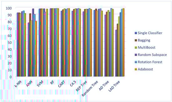
Figure 1.
Classification accuracies of machine learning methods as single classifiers and in combination with one of five ensemble machine learning methods.
Table A1, Table A2, Table A3, Table A4, Table A5 and Table A6 in the Appendix A present confusion matrices for different types of ensemble machine learning methods (see Appendix A).
Random Forest gave the best result for focal signals classification, and this result was satisfactory (Appendix A Table A1, 989 out of 1000). Using this method, there were only 11 false-negatives, which is great result, also considering only 15 false-positives. On the other hand, the lowest accuracy for the classification of non-focal signals was achieved using the ANN method, 775 out of 1000 (Appendix A Table A1), with similar results for focal signal classification. That means that ANN produces more than 200 false classifications (either focal or non-focal), which is a really big number.
Looking more at Appendix A Table A1, SVM gave one of the best results, with 13 false-negatives and 21 false-positives, and it was nearest to the performance of Random Forest. Appendix A Table A1 also shows that single machine learning methods usually produce better accuracy values for focal signal classification.
The only two algorithms that were better in non-focal signal classification were k-NN and LAD Tree. In addition, LAD Tree had the biggest difference between true-positives and true-negatives, 408 compared to 944, respectively.
4. Discussion
The proposed technique that includes MSPCA de-noising of EEG signals and spectral feature calculation using AR Burg, proved to be an adequate approach for discrimination of non-focal and focal EEG signals.
Based on the presented results, emphasis on the following could be stated:
- Random Forest was the best performer as a single classifier or when combined with one of the following three ensemble methods: Bagging, MultiBoost, and Random Subspace, with accuracy around 98.7%.
- Even if it is the best machine learning technique among the four methods, Random Forest did not give the best overall accuracy.
- REP Tree achieved the best result in combination with the Rotation Forest method among all methods and classifiers, with accuracy of 98.9%.
- ANN and LAD Tree were the worst performing methods. No matter which ensemble machine learning method was used, or in a single classifier scenario, one of them gave the worst results.
- In the case of the Random Subspace ensemble method, we can see that there is a very small difference between the best and the worst performing technique. This means that the accuracy of good-performing algorithms did not change by much, but bad single performers became much better. This was clearly visible in the 92.85% accuracy for LAD Tree as the worst technique, and the best technique being the Random Forest, with accuracy of 98.65%. Therefore, we can state that Random Subspace could be proposed as the most effective and robust ensemble method, because it managed to reach accuracies higher than 92% for all single classifiers (even though the biggest accuracies were reached by other ensembles).
- Although LAD Tree was one of the worst proposed machine learning techniques in this study, the AdaBoost ensemble method with LAD Tree as a base classifier reached a very high total accuracy of 98.75%. It really shows how ensembles can improve the accuracy of a base classifier by a significant margin.
- Results in Table 1 and Table 2 show that Random Forest was the most robust single machine learning technique in combination with any of the proposed ensemble methods, hence it could be successfully used in EEG signals’ classification for the epileptic focal region localization. On the other hand, we can see that Rotation Forest could be considered as the best proposed ensemble method because it achieved the highest accuracy with REP Tree and no accuracy value below 90%.
- In the case of the k-NN classifier, we can observe that the difference between the best and the worst accuracy as a single classifier or in a combination with ensemble machine learning methods was 3.55% (the best was 95.25%, the worst was 91.7%). It means that one classifier in different ensemble combination can produce almost the same accuracy. A similar situation can be seen with RF, CART, and SVM.
- The AUC value of Rotation Forest and REP Tree, as the best achieved method, was 0.999, and it would be considered to be “good” at separating non-focal and focal signals.
To further emphasize the importance of our findings, our results were compared to several previous studies in the state-of-the-art applied on the same dataset using machine learning. This shows that our idea is novel as small numbers of scientists have dealt with the issue of localization of non-focal and focal brain regions.
The most promising results have been achieved by Sharma et al. [45], who incorporated Least Squares Support Vector Machine (LS-SVM) on wavelet entropy attributes to achieve 94.25% accuracy. Using the same classifier, Bhattacharyya et al. [46] reached no more than 90% accuracy. On the other hand, Zhu et al. [47] reached no more than 84% accuracy with SVM applied together with delay permutation entropy as a feature-selection mechanism. Das et al. [48] showed another promising result, with more than 90% of accuracy when Empirical Mode Decomposition (EMD) and Discrete Wavelet Transform (DWT) were used as attribute extractors for SVM and k-NN. In our previous studies [6], we presented the approach of choosing the optimal attribute extraction technique for classification of non-focal and focal EEG signals, where time-consuming Wavelet Packet Decomposition (WPD) attributes reached the accuracy of 99.92% with Random Forest. In this study, the idea was to use a simpler feature extraction algorithm (AR Burg) coupled with more complex ensemble machine learning algorithms (which were not the focus in Reference [6]), which helped us achieve the accuracy of 98.9%. These results demonstrate that our suggested approach outperforms previous studies by other authors.
5. Conclusions
The EEG signal visual analysis is not a successful way to distinguish focal from non-focal signals. On the other hand, an approach based on the machine learning methods is capable of dealing with a task of epileptic focal region localization. We covered machine learning and introduced ensemble machine learning techniques (Bagging, Boosting, AdaBoost, MultiBoost, Random Subspace Method, and Rotation Forest).
In this experiment, epileptic focal region localization was presented by incorporating the MSPCA de-noising algorithm. The AR Burg method was applied to generate the power spectral density (PSD) of de-noised EEG signals. PSD values were fed as inputs to five machine learning techniques, with which its performance was evaluated according to the following three criteria: accuracy, AUC, and F-measure. In this research, EEG signals were preprocessed using the MSPCA to decrease the noise. AR Burg algorithms were responsible for feature extraction from time to frequency domain. Ensemble machine learning methods were being fed with these features to recognize the changes in each segment of the brain during the onset of a seizure. The localization of epileptic regions was then compared to real brain location defined by the medical neurosurgeons.
In the experimental part of this paper, we presented the performance for different evaluation criteria used in this paper for ten machine learning techniques, which were used in combination with a single classifier and five different ensemble machine learning techniques. According to the results of the experiment, the brain regions which contain epileptic focus are easier to identify than non-focal regions.
From this result, majority of machine learning methods produced better accuracy for focal signals than for non-focal signals, with only LAD Tree and k-NN to disapprove. Random Forest gave the best result for focal signals’ classification, and this result was satisfactory (Appendix A Table A1, 989 out of 1000). Using this method, there were only 11 false-negatives, which is a great result, also considering only 15 false-positives. On the other hand, the lowest accuracy for the classification of non-focal signals was achieved using the ANN method, at 775 out of 1000 (Appendix A Table A1), with similar results for focal signal classification. That means ANN produced more than 200 false classifications (either focal or non-focal), which is a really big number.
This estimation can be useful in localization of the epileptic focus region. The focus region of patients which was used in this experiment was classified, up to 99%, so the result of classification using different machine learning techniques in combination with different ensemble methods shows that de-noised signal using MSPCA achieved efficient classification accuracy. Therefore, the suggested technique can be of potential application for defining the epilepsy focus region in the brain according to the EEG signals’ analysis from the scalp.
Our further research may relate to combining the proposed approach with ensemble machine learning and hybrid networks of evolutionary processors and networks of splicing processors [49,50]. Also, one can discuss about linking the proposed approach and a new type of uniformly bounded duplication language, based on bio-inspired computation in the evolution of DNA [51].
Author Contributions
Formal analysis, S.J. and M.S.; investigation, S.J., M.S., A.S., and J.K.; Methodology, S.J. All authors have read and agreed to the published version of the manuscript.
Funding
This research received no external funding.
Conflicts of Interest
The authors declare no conflict of interest.
Appendix A
Table A1, Table A2, Table A3, Table A4, Table A5 and Table A6 present confusion matrices for different types of machine learning ensemble methods (Single Classifier, Bagging, MultiBoost, Random Subspace, Rotation Forest, and AdaBoost).
Table A1.
Confusion matrix for Single Classifier.
Table A1.
Confusion matrix for Single Classifier.
| ML Method | K-NN | ANN | SVM | RF | CART | |||||
|---|---|---|---|---|---|---|---|---|---|---|
| Actual/Predict | Focal | Non-Focal | Focal | Non-Focal | Focal | Non-Focal | Focal | Non-Focal | Focal | Non-Focal |
| Focal | 922 | 71 | 785 | 225 | 987 | 21 | 989 | 15 | 957 | 54 |
| Non-focal | 78 | 929 | 215 | 775 | 13 | 979 | 11 | 985 | 43 | 946 |
| ML Method | C4.5 | REP Tree | Random Tree | AD Tree | LAD Tree | |||||
| Actual/Predict | Focal | Non-focal | Focal | Non-focal | Focal | Non-focal | Focal | Non-focal | Focal | Non-focal |
| Focal | 964 | 54 | 942 | 59 | 964 | 39 | 929 | 139 | 408 | 56 |
| Non-focal | 36 | 946 | 58 | 941 | 36 | 961 | 71 | 861 | 592 | 944 |
Table A2.
Confusion matrix for Bagging.
Table A2.
Confusion matrix for Bagging.
| ML Method | K-NN | ANN | SVM | RF | CART | |||||
|---|---|---|---|---|---|---|---|---|---|---|
| Actual/Predict | Focal | Non-Focal | Focal | Non-Focal | Focal | Non-Focal | Focal | Non-Focal | Focal | Non-Focal |
| Focal | 921 | 71 | 921 | 94 | 989 | 21 | 988 | 15 | 974 | 31 |
| Non-focal | 79 | 929 | 79 | 906 | 11 | 979 | 12 | 985 | 26 | 969 |
| ML Method | C4.5 | REP Tree | Random Tree | AD Tree | LAD Tree | |||||
| Actual/Predict | Focal | Non-focal | Focal | Non-focal | Focal | Non-focal | Focal | Non-focal | Focal | Non-focal |
| Focal | 973 | 20 | 977 | 23 | 981 | 17 | 950 | 76 | 565 | 37 |
| Non-focal | 27 | 980 | 23 | 977 | 19 | 983 | 50 | 924 | 435 | 963 |
Table A3.
Confusion matrix for MultiBoost.
Table A3.
Confusion matrix for MultiBoost.
| ML Method | K-NN | ANN | SVM | RF | CART | |||||
|---|---|---|---|---|---|---|---|---|---|---|
| Actual/Predict | Focal | Non-Focal | Focal | Non-Focal | Focal | Non-Focal | Focal | Non-Focal | Focal | Non-Focal |
| Focal | 916 | 82 | 816 | 192 | 987 | 22 | 988 | 15 | 986 | 15 |
| Non-focal | 84 | 918 | 184 | 808 | 13 | 978 | 12 | 985 | 14 | 985 |
| ML Method | C4.5 | REP Tree | Random Tree | AD Tree | LAD Tree | |||||
| Actual/Predict | Focal | Non-focal | Focal | Non-focal | Focal | Non-focal | Focal | Non-focal | Focal | Non-focal |
| Focal | 989 | 18 | 975 | 16 | 958 | 48 | 960 | 39 | 832 | 93 |
| Non-focal | 11 | 982 | 25 | 984 | 42 | 952 | 40 | 961 | 168 | 907 |
Table A4.
Confusion matrix for Random Subspace.
Table A4.
Confusion matrix for Random Subspace.
| ML Method | K-NN | ANN | SVM | RF | CART | |||||
|---|---|---|---|---|---|---|---|---|---|---|
| Actual/Predict | Focal | Non-Focal | Focal | Non-Focal | Focal | Non-Focal | Focal | Non-Focal | Focal | Non-Focal |
| Focal | 950 | 64 | 985 | 18 | 986 | 19 | 988 | 15 | 974 | 24 |
| Non-focal | 50 | 936 | 15 | 982 | 14 | 981 | 12 | 985 | 26 | 976 |
| ML Method | C4.5 | REP Tree | Random Tree | AD Tree | LAD Tree | |||||
| Actual/Predict | Focal | Non-focal | Focal | Non-focal | Focal | Non-focal | Focal | Non-focal | Focal | Non-focal |
| Focal | 987 | 21 | 975 | 20 | 984 | 23 | 961 | 93 | 930 | 73 |
| Non-focal | 13 | 979 | 25 | 980 | 16 | 977 | 39 | 907 | 70 | 927 |
Table A5.
Confusion matrix for Rotation Forest.
Table A5.
Confusion matrix for Rotation Forest.
| ML Method | K-NN | ANN | SVM | RF | CART | |||||
|---|---|---|---|---|---|---|---|---|---|---|
| Actual/Predict | Focal | Non-Focal | Focal | Non-Focal | Focal | Non-Focal | Focal | Non-Focal | Focal | Non-Focal |
| Focal | 959 | 54 | 906 | 99 | 939 | 66 | 992 | 15 | 989 | 15 |
| Non-focal | 41 | 946 | 94 | 901 | 61 | 934 | 8 | 985 | 11 | 985 |
| ML Method | C4.5 | REP Tree | Random Tree | AD Tree | LAD Tree | |||||
| Actual/Predict | Focal | Non-focal | Focal | Non-focal | Focal | Non-focal | Focal | Non-focal | Focal | Non-focal |
| Focal | 992 | 15 | 993 | 15 | 986 | 15 | 993 | 15 | 982 | 22 |
| Non-focal | 8 | 985 | 7 | 985 | 14 | 985 | 7 | 985 | 18 | 978 |
Table A6.
Confusion matrix for AdaBoost.
Table A6.
Confusion matrix for AdaBoost.
| ML Method | K-NN | ANN | SVM | RF | CART | |||||
|---|---|---|---|---|---|---|---|---|---|---|
| Actual/Predict | Focal | Non-Focal | Focal | Non-Focal | Focal | Non-Focal | Focal | Non-Focal | Focal | Non-Focal |
| Focal | 916 | 82 | 920 | 317 | 984 | 23 | 991 | 16 | 991 | 15 |
| Non-focal | 84 | 918 | 80 | 683 | 16 | 977 | 9 | 984 | 9 | 985 |
| ML Method | C4.5 | REP Tree | Random Tree | AD Tree | LAD Tree | |||||
| Actual/Predict | Focal | Non-focal | Focal | Non-focal | Focal | Non-focal | Focal | Non-focal | Focal | Non-focal |
| Focal | 984 | 22 | 977 | 23 | 956 | 50 | 979 | 23 | 988 | 13 |
| Non-focal | 16 | 978 | 23 | 977 | 44 | 950 | 21 | 977 | 12 | 987 |
References
- Gevins, A.; Remond, A. Handbook of EEG and Clinical Neurophysiology; Elsevier: Amsterdam, The Netherlands, 1987. [Google Scholar]
- Swiderski, B.; Osowski, S.; Cichocki, A.; Rysz, A. Single-Class SVM Classifier for Localization of Epileptic Focus on the Basis of EEG. In Proceedings of the International Joint Conference on Neural Networks, Hong Kong, China, 1–8 June 2008. [Google Scholar]
- Xiaoying, T.; Li, X.; Weifeng, L.; Yuhua, P.; Duanduan, C.; Tianxin, G.; Yanjun, Z. Analysis of Frequency Domain of EEG Signals in Clinical Location of Epileptic Focus. Clin. EEG Neurosci. 2013, 44, 25–30. [Google Scholar]
- Stam, C.J. Nonlinear dynamical analysis of EEG and MEG: Review of an emerging field. Clin. Neurophysiol 2005, 116, 2266–2301. [Google Scholar] [CrossRef] [PubMed]
- Pereda, E.; Quian Quiroga, R.; Bhattacharya, J. Nonlinear multivariate analysis of neurophysiological signals. Prog. Neurobiol. 2005, 77, 1–37. [Google Scholar] [CrossRef]
- Subasi, A.; Jukic, S.; Kevric, J. Comparison of EMD, DWT and WPD for the localization of epileptogenic foci using Random Forest classifier. Measurement 2019, 146, 846–855. [Google Scholar] [CrossRef]
- Pedro, C.E.; Joyce, W.Y.; Leo, C.L.; Kirk, S.; Sandy, D.; Marc, N.R. Quantification and localization of EEG interictal spike activity in patients with surgically removed epileptogenic foci. Clin. Neurophysiol. 2012, 123, 471–485. [Google Scholar]
- Ochi, A.; Otsubo, H.; Shirasawa, A.; Hunjan, A.; Sharm, R.; Bettings, M. Systematic approch to dipole localization of interictal EEG spikes in children with extratemporal lobe epilepsy. Clin. Neurophysiol. 2000, 111, 161–168. [Google Scholar] [CrossRef]
- Wilson, S.B.; Turner, C.A.; Emerson, R.G.; Scheuer, M.L. Spike detection II: Automatic, perception-based detection and clustering. Clin. Neurophysiol. 1999, 110, 404–411. [Google Scholar] [CrossRef]
- Bakshi, B.R. Multiscale PCA with Application to Multivariate Statistical Process Monitoring. AIChE J. 2004, 44, 1596–1610. [Google Scholar] [CrossRef]
- Gokgoz, E.; Subasi, A. Effect of Multiscale PCA de-noising on EMG signal classification for Diagnosis of Neuromuscular Disorders. J. Med. Syst. 2014, 38, 1–10. [Google Scholar] [CrossRef]
- Jackson, J.E. A User’s Guide to Principal Components; John Wiley: New York, NY, USA, 1991. [Google Scholar]
- Malinowski, E.R. Factor Analysis in Chemistry; John Wiley: New York, NY, USA, 1991. [Google Scholar]
- Sornmo, L.; Laguna, P. Bioelectrical Signal Processing in Cardiac and Neurological Application; Elsevier: Amsterdam, The Netherlands, 2005. [Google Scholar]
- Ralph, A.G.; Kaspar, S.; Rummel, C. Nonrandomness, nonlinear dependence, and nonstationarity of electroencephalographic. Phys. Rev. E 2012, 86, 1–8. [Google Scholar]
- Swiderski, B.; Osowski, S.; Cichocki, A.; Rysz, A. Epileptic seizure characterization by Lyapunov exponent of EEG signal. COMPEL Int. J. Comput. Math. Electr. Electron. Eng. 2007, 26, 1276–1287. [Google Scholar]
- Jäntschi, L. The Eigenproblem Translated for Alignment of Molecules. Symmetry 2019, 11, 1027. [Google Scholar] [CrossRef]
- Holhoş, A.; Roşca, D. Orhonormal Wavelet Bases on The 3D Ball Via Volume Preserving Map from the Regular Octahedron. Mathematics 2020, 8, 994. [Google Scholar] [CrossRef]
- Kevric, J.; Subasi, A. The impact of Mspca signal de-noising in real-time wireless brain computer interface system. Southeast Eur. J. Soft Comput. 2015, 4, 43–47. [Google Scholar] [CrossRef]
- Lehnertz, K. Epilepsy and Nonlinear Dynamics. J. Biol. Phys. 2008, 34, 253–266. [Google Scholar] [CrossRef]
- Adeli, H.; Zhou, Z.; Dadmehr, N. Analysis of EEG records in an epileptic patient using wavelet transform. J. Neurosci. Methods 2003, 123, 69–87. [Google Scholar] [CrossRef]
- Cohen, A. Biomedical Signals: Origin and Dynamic Characteristics. In Frequency-Domain Analysis, 2nd ed.; CRC Press LLC: Boca Raton, FL, USA, 2000. [Google Scholar]
- Muthuswamy, J.; Thakor, N.V. Spectral analysis methods for neurological signals. J. Neurosci. Methods 1998, 83, 1–14. [Google Scholar] [CrossRef]
- Goto, S.; Nakamura, M.; Uosaki, K. On-line spectral estimation of nonstationary time series based on AR model parameter estimation and order selection with a forgetting factor. IEEE Trans. Signal Process. 1995, 43, 1519–1522. [Google Scholar] [CrossRef]
- Rezaul, B.; Daniel, L.T.H.; Marimuthu, P. Computational Intelligence in Biomedical Engineering; CRC Press: Boca Raton, FL, USA, 2007. [Google Scholar]
- Subasi, A.; Erçelebi, E.; Alkan, A.; Koklukaya, E. Comparison of subspace-based methods with AR parametric methods in epileptic seizure detection. Comput. Biol. Med. 2006, 36, 195–208. [Google Scholar] [CrossRef]
- William, P.; Qin, D.; Anne, D. Lazy Classifiers Using P-trees. In Proceedings of the 15th International Conference on Computer Applications in Industry and Engineering, Clarion Hotel Bay View, San Diego, CA, USA, 7–9 November 2002. [Google Scholar]
- Browne, M.; Berry, M.M. Lecture Notes in Data Mining; World Scientific Publishing: Singapore, 2006. [Google Scholar]
- Pardey, J.; Roberts, S.; Tarassenko, L. A review of parametric modelling techniques for EEG analysis. Med. Eng. Phys. 1996, 18, 2–11. [Google Scholar] [CrossRef]
- Cristianini, N.; Shave-Taylor, J. An Introduction to Support Vector Machines: And Other Kernel-Based Learning Methods; Cambridge University Press: New York, NY, USA, 2000. [Google Scholar]
- Hall, M.; Witten, I.; Frank, E. Data Mining: Practical Machine Learning Tools and Techniques; Kaufmann: Burlington, NJ, USA, 2011. [Google Scholar]
- Vapnik, V.N. The Nature of Statisical Learning Theory, 2nd ed.; Springer: New York, NY, USA, 2000. [Google Scholar]
- Dunham, M. Data Mining: Introductory and Advanced Topics; Prentece Hall: Upper Saddle River, NJ, USA, 2003. [Google Scholar]
- Breiman, L.; Friedman, J.H.; Olshen, R.A.; Stone, C.J. Classification and Regression Trees; Hall/CRC: Boca Raton, FL, USA, 1984. [Google Scholar]
- Breiman, L. Random forest. Mach. Learn. 2001, 45, 5–32. [Google Scholar] [CrossRef]
- Fraiwana, L.; Lweesyb, K.; Khasawnehc, N.; Wendz, H.; Dickhause, H. Automated sleep stage identification system based on time-frequency of single EEG channel and random forest classifier. Comput. Methods Progr. Biomed. 2012, 108, 10–19. [Google Scholar] [CrossRef] [PubMed]
- Jäntschi, L.; Bolboacă, S.D. Performances of Shannon’s Entropy Statistic in Assessment of Distribution of Data. Ovidius Univ. Ann. Chem. 2017, 28, 30–42. [Google Scholar] [CrossRef]
- Kalmegh, S. Analysis of WEKA data mining algorithm REPTree, Simple CART and RandomTree for classification of Indian news. Int. J. Innov. Sci. Eng. Technol. 2015, 2, 438–460. [Google Scholar]
- Bauer, E.; Kohavi, R. An empirical comparison of voting classification algorithms: Bagging, boosting, and variants. Mach. Learn. 1999, 36, 105–139. [Google Scholar] [CrossRef]
- Webb, G.I. Multiboosting: A technique for combining boosting and wagging. Mach. Learn. 2000, 40, 159–196. [Google Scholar] [CrossRef]
- Rodríguez, J.; Kuncheva, L.; Alonso, C. Rotation forest: A new classifier ensemble method. IEEE Trans. Pattern Anal. Mach. Intell. 2006, 28, 1619–1630. [Google Scholar] [CrossRef]
- Ho, T.K. The random subspace method for constructing decision forests. IEEE Trans. Pattern Anal. Mach. Intell. 1998, 20, 832–844. [Google Scholar]
- Skurichina, M.; Duin, R.P. Bagging, boosting and the random subspace method for linear classifiers. Pattern Anal. Appl. 2002, 5, 121–135. [Google Scholar] [CrossRef]
- Frank, E.; Hall, M.A.; Witten, I.H. The WEKA Workbench: Online Appendix for Data Mining: Practical Machine Learning Tools and Techniques; Morgan Kaufmann: Burlington, NJ, USA, 2016. [Google Scholar]
- Sharma, M.; Dhere, A.; Pachori, R.B.; Acharya, U.R. An automatic detection of focal EEG signals using new class of time-frequency localized orthogonal wavelet filter banks. Knowl. Based Syst. 2016, 118, 217–227. [Google Scholar] [CrossRef]
- Bhattacharyya, A.; Sharma, M.; Pachori, R.; Sircar, P.; Acharya, U. A novel approach for automated detection of focal EEG signals using empirical wavelet transform. Neural Comput. Appl. 2018, 29, 47–57. [Google Scholar] [CrossRef]
- Zhu, G.; Li, Y.; Wen, P.; Wang, S.; Xi, M. Epileptogenic focus detection in intracranial EEG based on delay permutation entropy. Proc. Am. Inst. Phys. 2013, 1559, 31–36. [Google Scholar]
- Das, A.; Bhuiyan, M. Discrimination and classification of focal and non-focal EEG signals using entropy-based features in the EMD-DWT domain. Biomed. Signal Process. Control 2016, 29, 11–21. [Google Scholar] [CrossRef]
- Manea, F.; Margenstern, M.; Mitrana, V.; Pérez-Jiménez, M.J. A New Characterization of NP, P, and PSPACE with Accepting Hybrid Networks of Evolutionary Processors. Theory Comput. Syst. 2010, 46, 174–192. [Google Scholar] [CrossRef]
- Manea, F.; Martín-Vide, C.; Mitrana, V. All NP-Problems Can Be Solved in Polynomial Time by Accepting Networks of Splicing Processors of Constant Size. In Proceedings of the International Workshop on DNA-Based Computers, Munich, Germany, 4–8 September 2016. [Google Scholar]
- Leupold, P.; Martín-Vide, C.; Mitrana, V. Uniformly bounded duplication languages. Discret. Appl. Math. 2005, 146, 301–310. [Google Scholar] [CrossRef]
© 2020 by the authors. Licensee MDPI, Basel, Switzerland. This article is an open access article distributed under the terms and conditions of the Creative Commons Attribution (CC BY) license (http://creativecommons.org/licenses/by/4.0/).