Some Inverse Source Problems of Determining a Space Dependent Source in Fractional-Dual-Phase-Lag Type Equations

Abstract

The dual-phase-lag heat transfer models attract a lot of interest of researchers in the last few decades. These are used in problems arising from non-classical thermal models, which are based on a non-Fourier type law. We study uniqueness of solutions to some inverse source problems for fractional partial differential equations of the Dual-Phase-Lag type. The source term is supposed to be of the form $h\left(t\right)f\left(\mathbf{x}\right)$ with a known function $h\left(t\right)$. The unknown space dependent source $f\left(\mathbf{x}\right)$ is determined from the final time observation. New uniqueness results are formulated in Theorem 1 (for a general fractional Jeffrey-type model). Here, the variational approach was used. Theorem 2 derives uniqueness results under weaker assumptions on $h\left(t\right)$ (monotonically increasing character of $h\left(t\right)$ was removed) in a case of dominant parabolic behavior. The proof technique was based on spectral analysis. Section Modified Model for ${\tau }_q>{\tau }_T$ shows that an analogy of Theorem 2 for dominant hyperbolic behavior (fractional Cattaneo–Vernotte equation) is not possible.

1. Introduction

The classical heat conduction theory is based on Fourier’s law, which yields infinite speed of thermal disturbances, which is nonphysical. On the other hand, non-classical models allow for a pertubation of the heat flux by a non-Fourier effect (additional term), cf. [1,2] As a consequence, a hyperbolic heat conduction model can be developed, and the propagation speed of heat will be finite. Cattaneo’s equation [1] in fact leads to the hyperbolic model described by the telegraph (or damped wave) equation. We consider models which allow perturbations for both the heat flux and temperature gradient, known as dual-phase-lag type equations.

1.1. Modeling

Let $\Omega \subset {\mathbb{R}}^d,d\in \mathbb{N}$ be a bounded domain with a Lipschitz continuous boundary $\partial \Omega$. The final time is denoted by $\mathcal{T}$ and we set $Q_{\mathcal{T}}:=\Omega \times (0,\mathcal{T}]$ and ${\Sigma }_{\mathcal{T}}:=\partial \Omega \times (0,\mathcal{T}]$. The classical Fourier law describes the relation between heat flux and temperature gradient as follows:

$$\mathbf{q}(\mathbf{x},t)=-k\left(\mathbf{x}\right)\nabla T(\mathbf{x},t)$$

where $\mathbf{x}$ is a material point, t is the time (in seconds (s)), k is the thermal conductivity (in W/(mK)) $\mathbf{q}$ is the heat flux (in W/m${}^2$), T stands for the temperature (in K), and ∇ is on behalf of the gradient operator. The minus sign “−” on the right side means that the direction of heat transmission goes from places with higher temperature to the ones with lower temperature.

The concept of Tzou [3] allows for the heat flux and the temperature gradient to occur at different instants of time in micro-scale heat transfer with relaxation time, see, e.g., [4]. This can be represented as a non-Fourier type law:

$$\mathbf{q}(\mathbf{x},t+{\tau }_q)=-k\left(\mathbf{x}\right)\nabla T(\mathbf{x},t+{\tau }_T),{\tau }_q>0,{\tau }_T>0,$$

(1)

where ${\tau }_q$ and ${\tau }_T$ are introduced as the phase-lag parameters (in seconds). Taking the first-order Taylor series expansion on both sides with reference to time t (neglecting the second- and higher-order terms) yields (This is a constitutive model of Jeffrey’s-type equation.)

$$\mathbf{q}(\mathbf{x},t)+{\tau }_q{\partial }_t\mathbf{q}(\mathbf{x},t)=-k\left(\mathbf{x}\right)\left(\nabla T(\mathbf{x},t)+{\tau }_T{\partial }_t\nabla T(\mathbf{x},t)\right),$$

which describes the classical Dual-Phase-Lag (DPL) heat conduction. Considering the fractional version of this relation, we replace the two first order derivatives with respect to time by the fractional operators, and the Phase-Lags ${\tau }_q$ and ${\tau }_T$ by ${\tau }_q^{\alpha }$ and ${\tau }_T^{\beta }$, which are introduced to maintain the dimensions in order. The time fractional Dual-Phase-Lag model then reads as (see [5])

$$\mathbf{q}(\mathbf{x},t)+{\tau }_q^{\alpha }{D}_t^{\alpha }\mathbf{q}(\mathbf{x},t)=-k\left(\mathbf{x}\right)\left(\nabla T(\mathbf{x},t)+{\tau }_T^{\beta }{D}_t^{\beta }\nabla T(\mathbf{x},t)\right).$$

(2)

The fractional derivative of order $\gamma$ is defined by

$$\left(D_t^{\gamma }u\right)(\mathbf{x},t):=\left(g_{1-\gamma }\ast u_t\left(\mathbf{x}\right)\right)\left(t\right)={\int }_0^t{g}_{1-\gamma }(t-s)u_t(\mathbf{x},s)\mathrm{d}s,$$

where the kernel $g_{1-\gamma }$ is defined by

$$g_{1-\gamma }\left(t\right)=\frac{t^{-\gamma }}{\Gamma (1-\gamma )},t>0,0<\gamma <1,$$

where $\Gamma$ denotes the Gamma function. The convolution term is the Caputo fractional derivative of order $\gamma \in (0,1),$ cf. [6]. Note that the Riemann–Liouville kernel $g_{1-\gamma }\in L_{\mathrm{loc}}^1(0,\infty )$ satisfies

$${(-1)}^j{g}_{1-\gamma }^{\left(j\right)}\left(t\right)\ge 0,\forall t\ge 0,j=0,1,2;g_{1-\gamma }^{\prime }\not\equiv 0,$$

and thus it is strongly positive definite by [7] Corollary 2.2. This means that

$${\int }_0^t(g_{1-\gamma }\ast y)\left(s\right)y\left(s\right)\mathrm{d}s\ge 0\forall t\ge 0,y\in L_{loc}^2\left((0,\infty )\right).$$

(3)

1.2. Derivation of the Source Term

Following the energy conservation law, it holds that

$$\rho c{\partial }_{t}T(\mathbf{x},t)+\nabla ·\mathbf{q}(\mathbf{x},t)=g(\mathbf{x},t),$$

(4)

where $\rho >0$ and $c>0$ are the density (in kg/m${}^3)$ and the specific heat of the material (in J/(K kg)) respectively, and g involves the source of heating. Combining Equation (2) with this, we arrive at the Fractional Dual-Phase-Lag (FDPL) heat equation in the form

$$\left(1+{\tau }_q^{\alpha }{D}_t^{\alpha }\right)\left(\rho c{\partial }_{t}T(\mathbf{x},t)\right)+\nabla ·\left(-k\left(\mathbf{x}\right)\left(\nabla T(\mathbf{x},t)+{\tau }_T^{\beta }{D}_t^{\beta }\nabla T(\mathbf{x},t)\right)\right)=\left(1+{\tau }_q^{\alpha }{D}_t^{\alpha }\right)g(\mathbf{x},t).$$

(5)

Let us have a closer look at the form of the source term, which depends on the situation under consideration. If we consider e.g., the temperature distribution inside living tissues subject to laser/electromagnetic radiation, then g has more components $g=g_b+g_M+g_s$, cf. [8,9]. The term $g_b$ represents a heat source due to blood circulation and it may be expressed as

$$g_b=W_b{C}_b(T_a-T),$$

where the constant $T_a$ stands for the arterial blood temperature, the blood perfusion coefficient $W_b$ represents the heat removal produced by the blood flow; and $C_b$ is the specific heat of blood. The heat generated per unit volume of tissue due to the absorption of electromagnetic radiation is represented by the term $g_s$. It depends only on the location of the antenna and its transmitting power P, which might be time-dependent and can be expressed as

$$g_s=\rho SP{e}^{\eta (p-r)},$$

where $S,\eta$ are constants, r is the position of the probe, and p is the depth of the material point. The source arising from metabolism has the form

$$g_M=g_m\left(1+\frac{T-T_0}{10}\right),$$

where $g_m$ is the reference metabolism and $T_0$ is the initial temperature. We see opposite sign before T at $g_b$ and $g_M$. Considering the physical values for blood (following [8]), we have $W_b=8$ kg m${}^{-3}$ s${}^{-1}$, $C_b=3344$ J kg${}^{-1}$ K${}^{-1}$, $T_0=T_a=37$${}^{\circ }$ C, $g_m=1091$ W m${}^{-3}$ = 1091 Jm${}^{-3}$ s${}^{-1}$, and we reveal that $W_b{C}_b>\frac{g_m}{10}$. Collecting, we may write for some known $a\ge 0,$

$$\left(1+{\tau }_q^{\alpha }{D}_t^{\alpha }\right)g(\mathbf{x},t)=F\left(\mathbf{x}\right)+f\left(\mathbf{x}\right)h\left(t\right)-a\left(1+{\tau }_q^{\alpha }{D}_t^{\alpha }\right)T(\mathbf{x},t).$$

(6)

Here, the external (antenna) source is considered in a separated form (space and time). By combining this relation with (5), we arrive at the final fractional form of Dual-Phase-Lag heat equation for $(\mathbf{x},t)\in Q_{\mathcal{T}},$

$$\begin{array}{cc}\hfill (1+{\tau }_q^{\alpha }{D}_t^{\alpha })\left(\rho c{\partial }_{t}T(\mathbf{x},t)\right)+a\left(1+{\tau }_q^{\alpha }{D}_t^{\alpha }\right)T(\mathbf{x},t)+\nabla ·(-k\left(\mathbf{x}\right)(\nabla T(\mathbf{x},t)& +{\tau }_T^{\beta }{D}_t^{\beta }\nabla T(\mathbf{x},t))\hfill \\ & =F\left(\mathbf{x}\right)+f\left(\mathbf{x}\right)h\left(t\right)\hfill \end{array}$$

(7)

subject to the initial data

$$T(\mathbf{x},0)=T_0\left(\mathbf{x}\right),{\partial }_{t}T(\mathbf{x},0)=V_0\left(\mathbf{x}\right),\mathbf{x}\in \Omega .$$

(8)

For ease of explanation, we consider Dirichlet boundary conditions (BCs)

$$T(\mathbf{x},t)=T_{\Gamma }(\mathbf{x},t),(\mathbf{x},t)\in {\Sigma }_{\mathcal{T}}.$$

(9)

Neumann and Robin/Newton type BCs can be handled in a similar way.

1.3. Existing Results of the Phase-Lag Type Models

Several papers are devoted to theoretical and numerical studies of phase-lag models considering the classical (not fractional) derivatives (i.e., $\alpha =1=\beta$ in (7)). Methods of solution regarding phase-lag models in one dimension have been discussed by Tzou [10]. More dimensions have been considered in [11]. Actually, the phase-lag models represent a special case of integrodifferential equations which have been intensively studied in the eighties of the 20th century. In fact, the relation (7) with classical derivatives reads as

$$\begin{array}{cc}\hfill \rho c{\partial }_{t}T(\mathbf{x},t)+{\tau }_q\rho c{\partial }_{tt}^{2}T(\mathbf{x},t)+a(T(\mathbf{x},t)+{\tau }_q{\partial }_{t}T(\mathbf{x},t))+\nabla ·(-k\left(\mathbf{x}\right)(\nabla T(\mathbf{x},t)& +{\tau }_T\nabla {\partial }_{t}T(\mathbf{x},t)\left)\right)\hfill \\ & {\displaystyle =F\left(\mathbf{x}\right)+f\left(\mathbf{x}\right)h\left(t\right).}\hfill \end{array}$$

(10)

This can be easily transformed into an integrodifferential equation

$$\begin{array}{c}\hfill {\displaystyle {\tau }_q\rho c{\partial }_{t}u(\mathbf{x},t)+\left(\rho c+a{\tau }_q\right)u(\mathbf{x},t)+\nabla ·\left(-k\left(\mathbf{x}\right){\tau }_T\nabla u(\mathbf{x},t)\right)}\\ \hfill {\displaystyle =\tilde{F}(\mathbf{x},t)+\nabla ·\left(k\left(\mathbf{x}\right)\left(\nabla {\int }_0^{t}u(\mathbf{x},s)\mathrm{d}s\right)\right)-a{\int }_0^{t}u(\mathbf{x},s)\mathrm{d}s,}\end{array}$$

(11)

where we put $T(\mathbf{x},t)=T_0\left(\mathbf{x}\right)+{\int }_0^{t}u(\mathbf{x},s)\mathrm{d}s$. Please note that ${\int }_0^{t}u(\mathbf{x},s)\mathrm{d}s$ represents a linear Volterra operator, cf. [12]. The equation (11) is a special case of an abstract parabolic semilinear equation with Volterra operators which has been studied in [13,14] (including full discretization). More general systems covering thermoelasticity problems with memory have been analyzed (well-posedness and regularity) in [15,16].

For the moment, we are not aware of references concerning the well-posedness and regularity of the multi-dimensional fractional Dual-Phase-Lag model (7); however, the suitable proof-technique is available in papers concerning fractional diffusion. The 1D solvability was treated in [5], where analytical solutions expressed by H-functions are obtained by using the Laplace and Fourier transforms method.

An inverse source problem (ISP) of determining a missing solely time-dependent function in a nonlinear parabolic integrodifferential setting has been studied in [17]. This covers the inverse source problem for determination of unknown $h\left(t\right)$ if the source is in a separated form $f\left(\mathbf{x}\right)h\left(t\right)$ as in the classical relation (10). Time-reversed models of inverse problems modeled by non-Fourier heat conduction law have been investigated by [18,19], in the non fractional case.

Higher-order approximations to the DPL model were studied in [20]. Solutions to the problems considered in this paper manifest unphysical behavior with negative values of temperature for ${\tau }_q>{\tau }_T$. A similar problem in the framework of the first-order approximation (for ${\tau }_q>{\tau }_T$) to the DPL model was studied in [21]. Exponential stability (based on relation between ${\tau }_T$ en ${\tau }_q$) of solutions with higher-order approximation to the DPL equation was studied in [22].

1.4. Organization of the Paper

We aim to analyze uniqueness results based on different assumptions on the known time-dependent term h of the source term. The paper is organized as follows: In Section 2, we show uniqueness of the inverse source problem of determining $f\left(\mathbf{x}\right)$ from the final time observation, cf. Theorem 1, by using the variational technique, supposing $h\left(t\right)>0,h^{\prime }\left(t\right)\ge 0$. To our best knowledge, this is the very first result of this type and the highlight for the fractional DPL equation. Next, we modify the model-based on a relation between the phase-lag parameters—in Section 3 and Section 4. In the case that ${\tau }_T>{\tau }_q$, the character of the governing equation is more parabolic and the assumptions in Theorem 1 can be relaxed, see Theorem 2, the proof of which relies on the spectral method, where we just assume $0\not\equiv h\ge 0$. Section 4 shows that, if ${\tau }_q>{\tau }_T$, the assumptions of Theorem 1 cannot be relaxed, see Remark 3. Notice that the case ${\tau }_T={\tau }_q$ is less interesting, since a change in time scale reduces the model to the classical version.

2. Uniqueness for Isp by Determination of $\mathit{F}\mathbf{\left(}\mathbf{x}\mathbf{\right)}$ from the Final Time Observation

The goal of this section is to study the uniqueness of solution $\left(T\right(\mathbf{x},t),f(\mathbf{x}\left)\right)$ to the ISP (7)–(9) along with a given final time observation $T(\mathbf{x},\mathcal{T})$. Due to the linearity of the problem, we have to show if

$$\begin{array}{ccc}\hfill {\displaystyle \left(1+{\tau }_q^{\alpha }{D}_t^{\alpha }\right)\left(\rho c{\partial }_{t}T(\mathbf{x},t)\right)+a\left(1+{\tau }_q^{\alpha }{D}_t^{\alpha }\right)T(\mathbf{x},t)}& & \\ \hfill {\displaystyle +\nabla ·\left(-k\left(\mathbf{x}\right)\left(\nabla T(\mathbf{x},t)+{\tau }_T^{\beta }{D}_t^{\beta }\nabla T(\mathbf{x},t)\right)\right)}& {\displaystyle =f\left(\mathbf{x}\right)h\left(t\right)}\hfill & {\displaystyle \mathrm{in}{Q}_{\mathcal{T}}}\hfill \\ \hfill {\displaystyle T(\mathbf{x},t)}& {\displaystyle =0}\hfill & {\displaystyle \mathrm{in}{\Sigma }_{\mathcal{T}}}\hfill \\ \hfill {\displaystyle T(\mathbf{x},0)}& {\displaystyle =0}\hfill & {\displaystyle \mathrm{in}\Omega }\hfill \\ \hfill {\displaystyle {\partial }_{t}T(\mathbf{x},0)}& {\displaystyle =0}\hfill & {\displaystyle \mathrm{in}\Omega }\hfill \\ \hfill {\displaystyle T(\mathbf{x},\mathcal{T})}& {\displaystyle =0}\hfill & {\displaystyle \mathrm{in}\Omega }\hfill \end{array}$$

(12)

then $T(\mathbf{x},t)=0=f\left(\mathbf{x}\right)$.

The following lemma states a simple consequence of (3). This will be used in the proof of Theorem 1.

Lemma 1.

Let $0<\alpha <1$ and ${\partial }_{t}v\in L_{loc}^2((0,\infty ),L^2(\Omega ))$, $v\left(0\right)=0$. Then, for any $\xi \ge 0$, we have

$${\int }_0^{\xi }\left(\left(D_t^{\alpha }v\right)\left(s\right),v\left(s\right)\right)\mathrm{d}s\ge 0.$$

Proof. 

It holds that $g_{\alpha }\ast g_{1-\alpha }=1$. An easy calculation yields

$$\begin{array}{cc}\hfill {\int }_0^{\xi }\left(\left(D_t^{\alpha }v\right)\left(s\right),v\left(s\right)\right)\mathrm{d}s& ={\int }_0^{\xi }\left(\left(g_{1-\alpha }\ast {\partial }_{t}v\right)\left(s\right),{\int }_0^s{\partial }_{t}v\left(y\right)\mathrm{d}y\right)\mathrm{d}s\hfill \\ & ={\int }_0^{\xi }\left(\left(g_{1-\alpha }\ast {\partial }_{t}v\right)\left(s\right),\left(1\ast {\partial }_{t}v\right)\left(s\right)\right)\mathrm{d}s\hfill \\ & ={\int }_0^{\xi }\left(\left(g_{1-\alpha }\ast {\partial }_{t}v\right)\left(s\right),\left((g_{\alpha }\ast g_{1-\alpha })\ast {\partial }_{t}v\right)\left(s\right)\right)\mathrm{d}s\hfill \\ & ={\int }_0^{\xi }\left(\left(g_{1-\alpha }\ast {\partial }_{t}v\right)\left(s\right),\left(g_{\alpha }\ast (g_{1-\alpha }\ast {\partial }_{t}v)\right)\left(s\right)\right)\mathrm{d}s\hfill \\ & \stackrel{\left(3\right)}{\ge }0.\hfill \end{array}$$

□

The following theorem deals with the uniqueness of a solution to the ISP for the FDPL equation.

Theorem 1

(Uniqueness ISP). Assume $0<\alpha ,\beta <1,a\ge 0$,

$$\left\{\begin{array}{ccc}\hfill {\displaystyle k\left(\mathbf{x}\right)}& {\displaystyle ={\left(k_{i,j}\left(\mathbf{x}\right)\right)}_{i,j=1,\dots ,d},}\hfill & {\displaystyle \mathbf{x}\in \Omega ,k=k^{\mathsf{T}},}\hfill \\ \hfill {\displaystyle k_{i,j}}& {\displaystyle \in L_{\infty }\left(\Omega \right),}\hfill & {\displaystyle i,j=1,\dots ,d,}\hfill \\ \hfill {\displaystyle {\xi }^T·k\xi }& {\displaystyle =\sum _{i,j=1}^d{k}_{i,j}\left(\mathbf{x}\right){\xi }_i{\xi }_j\ge \underline{k}{\left|\xi \right|}^2,}\hfill & {\displaystyle \underline{k}>0,\forall \xi \in {\mathbb{R}}^d}\hfill \end{array}\right.$$

(13)

and $\rho ,c>0$ and $a,{\tau }_q^{\alpha },{\tau }_T^{\beta }\ge 0$. Moreover, suppose that $h\in C\left(\right[0,\mathcal{T}\left]\right)$, $h^{\prime }\in C\left((0,\mathcal{T}]\right)$ and

$$h\left(t\right)>0,h^{\prime }\left(t\right)\ge 0.$$

Presume that $\left(T\right(\mathbf{x},t),f(\mathbf{x}\left)\right)$ obeys (12) along with $T\in C\left([0,\mathcal{T}],H_0^1(\Omega )\right)$, ${\partial }_{t}T\in L^2\left((0,\mathcal{T}),L^2(\Omega )\right)$ and $f\in L^2(\Omega )$. Then, $T(\mathbf{x},t)=0=f\left(\mathbf{x}\right)$.

Proof. 

The variational formulation of the governing fractional partial differential equation (FPDE) reads as

$$\rho c\left({\partial }_{t}T,\phi \right)+\rho c{\tau }_q^{\alpha }\left(D_t^{\alpha }{\partial }_{t}T,\phi \right)+a\left(\left(1+{\tau }_q^{\alpha }{D}_t^{\alpha }\right)T,\phi \right)+\left(k\nabla T,\nabla \phi \right)+{\tau }_T^{\beta }\left(k{D}_t^{\beta }\nabla T,\nabla \phi \right)=h\left(t\right)\left(f,\phi \right)$$

for any $\phi \in H_0^1(\Omega )$.

Let us denote $H\left(t\right)=\frac{1}{h\left(t\right)}$. Then, we have $H^{\prime }\left(t\right)=-\frac{h^{\prime }\left(t\right)}{h^2\left(t\right)}\le 0$. Now, we divide the variational form by $h\left(t\right)$, set $\phi ={\partial }_{t}T$ and integrate over $[0,\mathcal{T}]$ to get

$$\begin{array}{c}\hfill {\displaystyle \rho c{\int }_0^{\mathcal{T}}H\left(s\right){∥{\partial }_{t}T\left(s\right)∥}^2\mathrm{d}s+\rho c{\tau }_q^{\alpha }{\int }_0^{\mathcal{T}}H\left(s\right)\left(\left(D_t^{\alpha }{\partial }_{t}T\right)\left(s\right),{\partial }_{t}T\left(s\right)\right)\mathrm{d}s}\\ \hfill {\displaystyle +{\int }_0^{\mathcal{T}}H\left(s\right)\left(aT\left(s\right),{\partial }_{t}T\left(s\right)\right)\mathrm{d}s+{\tau }_q^{\alpha }{\int }_0^{\mathcal{T}}H\left(s\right)\left(a\left(D_t^{\alpha }T\right)\left(s\right),{\partial }_{t}T\left(s\right)\right)\mathrm{d}s}\\ \hfill {\displaystyle +{\int }_0^{\mathcal{T}}H\left(s\right)\left(k\nabla T\left(s\right),\nabla {\partial }_{t}T\left(s\right)\right)\mathrm{d}s+{\tau }_T^{\beta }{\int }_0^{\mathcal{T}}H\left(s\right)\left(k{D}_t^{\beta }\nabla T\left(s\right),\nabla {\partial }_{t}T\left(s\right)\right)\mathrm{d}s=0,}\end{array}$$

since

$${\int }_0^{\mathcal{T}}\left(f,{\partial }_{t}T\left(s\right)\right)\mathrm{d}s=\left(f,{\int }_0^{\mathcal{T}}{\partial }_{t}T\left(s\right)\mathrm{d}s\right)=\left(f,T\left(\mathcal{T}\right)-T\left(0\right)\right)=0.$$

We can write using integration by parts in time

$$\begin{array}{cc}\hfill a{\int }_0^{\mathcal{T}}H\left(s\right)\left(T\left(s\right),{\partial }_{t}T\left(s\right)\right)\mathrm{d}s& =\frac{a}{2}{\int }_0^{\mathcal{T}}H\left(s\right){\partial }_s{∥T\left(s\right)∥}^2\mathrm{d}s\hfill \\ & =\frac{a}{2}{\left.H\left(s\right){∥T\left(s\right)∥}^2\right|}_{s=0}^{s=\mathcal{T}}-\frac{a}{2}{\int }_0^{\mathcal{T}}{H}^{\prime }\left(s\right){∥T\left(s\right)∥}^2\mathrm{d}s\hfill \\ & \ge 0,\hfill \end{array}$$

and

$$\begin{array}{cc}\hfill {\displaystyle {\int }_0^{\mathcal{T}}H\left(s\right)\left(\left(D_t^{\alpha }{\partial }_{t}T\right)\left(s\right),{\partial }_{t}T\left(s\right)\right)\mathrm{d}s}& {\displaystyle ={\left.H\left(t\right){\int }_0^t\left(\left(D_t^{\alpha }{\partial }_{t}T\right)\left(s\right),{\partial }_{t}T\left(s\right)\right)\mathrm{d}s\right|}_{t=0}^{t=\mathcal{T}}}\hfill \\ & {\displaystyle -{\int }_0^{\mathcal{T}}{H}^{\prime }\left(s\right){\int }_0^s\left(\left(D_t^{\alpha }{\partial }_{t}T\right)\left(\xi \right),{\partial }_{t}T\left(\xi \right)\right)\mathrm{d}\xi \mathrm{d}s}\hfill \\ & {\displaystyle =H\left(\mathcal{T}\right){\int }_0^{\mathcal{T}}\left(\left(D_t^{\alpha }{\partial }_{t}T\right)\left(s\right),{\partial }_{t}T\left(s\right)\right)\mathrm{d}s}\hfill \\ & {\displaystyle -{\int }_0^{\mathcal{T}}{H}^{\prime }\left(s\right){\int }_0^s\left(\left(D_t^{\alpha }{\partial }_{t}T\right)\left(\xi \right),{\partial }_{t}T\left(\xi \right)\right)\mathrm{d}\xi \mathrm{d}s}\hfill \\ & {\displaystyle \stackrel{\mathit{Lemma} 1}{\ge }0.}\hfill \end{array}$$

Furthermore,

$$\begin{array}{cc}\hfill {\displaystyle a{\int }_0^{\mathcal{T}}H\left(s\right)\left(\left(D_t^{\alpha }T\right)\left(s\right),{\partial }_{t}T\left(s\right)\right)\mathrm{d}s}& {\displaystyle =a{\left.H\left(t\right){\int }_0^t\left(\left(D_t^{\alpha }T\right)\left(s\right),{\partial }_{t}T\left(s\right)\right)\mathrm{d}s\right|}_{t=0}^{t=\mathcal{T}}}\hfill \\ & {\displaystyle -a{\int }_0^{\mathcal{T}}{H}^{\prime }\left(s\right){\int }_0^s\left(\left(D_t^{\alpha }T\right)\left(\xi \right),{\partial }_{t}T\left(\xi \right)\right)\mathrm{d}\xi \mathrm{d}s}\hfill \\ & {\displaystyle \stackrel{\mathit{Lemma} 1}{\ge }0,}\hfill \end{array}$$

$$\begin{array}{cc}\hfill {\displaystyle 2{\int }_0^{\mathcal{T}}H\left(s\right)\left(k\nabla T\left(s\right),\nabla {\partial }_{t}T\left(s\right)\right)\mathrm{d}s}& {\displaystyle ={\int }_0^{\mathcal{T}}H\left(s\right){\partial }_t\left(k\nabla T\left(s\right),\nabla T\left(s\right)\right)\mathrm{d}s}\hfill \\ & {\displaystyle ={\left.H\left(t\right)\left(k\nabla T\left(t\right),\nabla T\left(t\right)\right)\right|}_{t=0}^{t=\mathcal{T}}-{\int }_0^{\mathcal{T}}{H}^{\prime }\left(s\right)\left(k\nabla T\left(s\right),\nabla T\left(s\right)\right)\mathrm{d}s,}\hfill \\ & {\displaystyle \ge 0}\hfill \end{array}$$

and

$$\begin{array}{cc}\hfill {\displaystyle {\int }_0^{\mathcal{T}}H\left(s\right)\left(k{D}_t^{\beta }\nabla T\left(s\right),\nabla {\partial }_{t}T\left(s\right)\right)\mathrm{d}s}& {\displaystyle ={\left.H\left(t\right){\int }_0^t\left(k{D}_t^{\beta }\nabla T\left(s\right),\nabla {\partial }_{t}T\left(s\right)\right)\mathrm{d}s\right|}_{t=0}^{t=\mathcal{T}}}\hfill \\ & {\displaystyle -{\int }_0^{\mathcal{T}}{H}^{\prime }\left(s\right){\int }_0^s\left(k{D}_t^{\beta }\nabla T\left(\xi \right),\nabla {\partial }_{t}T\left(\xi \right)\right)\mathrm{d}\xi \mathrm{d}s}\hfill \\ & {\displaystyle \stackrel{\mathit{Lemma} 1}{\ge }0.}\hfill \end{array}$$

Summarizing all estimates above, we arrive at

$${\int }_0^{\mathcal{T}}H\left(s\right){∥{\partial }_{t}T\left(s\right)∥}^2\mathrm{d}s\le 0,$$

which implies $T(\mathbf{x},t)=0$ and consequently $f\left(\mathbf{x}\right)=0$ from the governing FPDE. □

Remark 1.

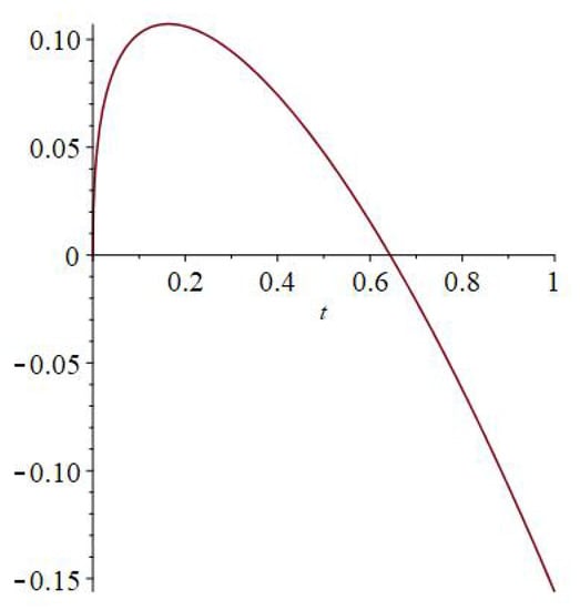
We show that the result of Theorem 1 is no longer true if the function h changes sign. Consider the following simplified form of (12):

$$\begin{array}{ccc}\hfill {\displaystyle \left(1+{\tau }_q^{\alpha }{D}_t^{\alpha }\right)\left({\partial }_{t}T(x,t)\right)-\left(1+{\tau }_T^{\beta }{D}_t^{\beta }\right)\Delta T(x,t)}& {\displaystyle =f\left(x\right)h\left(t\right)}\hfill & {\displaystyle in{Q}_{\mathcal{T}}}\hfill \\ \hfill {\displaystyle T(x,t)}& {\displaystyle =0}\hfill & {\displaystyle in{\Sigma }_{\mathcal{T}}}\hfill \\ \hfill {\displaystyle T(x,0)}& {\displaystyle =0}\hfill & {\displaystyle in\Omega ,}\hfill \\ \hfill {\displaystyle T(x,\mathcal{T})}& {\displaystyle =0}\hfill & {\displaystyle in\Omega ,}\hfill \end{array}$$

(14)

where $\Omega =(0,\pi )$ and $\mathcal{T}=1.$ The ISP for missing $f\left(x\right)$ has the trivial solution $\left(T\right(x,t),f(x\left)\right)=(0,0).$ We now determine a non-trivial solution, based on a modification of [23] Example 3.1. Take a function $g\left(x\right)$ such that $-\Delta g=\lambda g$ with $g\left(0\right)=g\left(\pi \right)=0$ and let $v\in C^2(0,1)$ with $v\left(0\right)=v\left(1\right).$ Set

$$h\left(t\right)={\tau }_q^{\alpha }(g_{1-\alpha }\ast v^{\prime \prime })\left(t\right)+\lambda {\tau }_T^{\beta }(g_{1-\beta }\ast v^{\prime })\left(t\right)+v^{\prime }\left(t\right)+\lambda v\left(t\right).$$

Then, we have the non-trivial solution $T(x,t)=v\left(t\right)g\left(x\right),f\left(x\right)=g\left(x\right)$ for example with $f\left(x\right)=sin\left(x\right)$, $\lambda =1$ and $v\left(t\right)=t^{\alpha +\beta +1}(1-t^b)$ where $b>0.$ We find

$$\begin{array}{cc}\hfill {\displaystyle h\left(t\right)}& {\displaystyle =\frac{{\tau }_q^{\alpha }}{\Gamma (1-\alpha )}\left(-(\alpha +\beta +b+1)(\alpha +\beta +b)t^{\beta +b}\mathrm{B}(\alpha +\beta +b,1-\alpha )\right.}\hfill \\ & {\displaystyle \left.+(\alpha +\beta )(\alpha +\beta +1)t^{\beta }\mathrm{B}(\alpha +\beta ,1-\alpha )\right)}\hfill \\ & {\displaystyle +\frac{\lambda {\tau }_T^{\beta }}{\Gamma (1-\beta )}\left(-(\alpha +\beta +b+1)t^{\alpha +1+b}\mathrm{B}(\alpha +\beta +b+1,1-\beta )\right.}\hfill \\ & {\displaystyle \left.+(\alpha +\beta +1)t^{\alpha +1}\mathrm{B}(\alpha +\beta +1,1-\beta )\right)}\hfill \\ & {\displaystyle +(\alpha +\beta +1)t^{\alpha +\beta }-(\alpha +\beta +b+1)t^{\alpha +\beta +b}+\lambda t^{\alpha +\beta +1}(1-t^b),}\hfill \end{array}$$

where $\mathrm{B}$ is the Beta function. The free parameters to tune are $\alpha ,\beta ,{\tau }_q,{\tau }_T,b$ and can be chosen in such a way that $h\left(t\right)$ changes its sign, see Figure 1.

Remark 2.

In Theorem 2 and Remark 3, we will use the real discrete spectrum of the self-adjoint positive differential operator $Av=\nabla ·(-k\nabla v)$ acting on e.g., $H_0^1(\Omega ),$ similar to the above (where k was the identity matrix). Performing the spectral analysis, this operator A has a real discrete spectrum $0<{\lambda }_n\to \infty ,$ with corresponding eigenfunctions $e_n\in H_0^1(\Omega ),$ which create an orthonormal base in $L^2(\Omega )$ and $A{e}_n={\lambda }_n{e}_n.$

3. Modified Model for ${\mathit{\tau }}_{\mathit{T}}\mathbf{>}{\mathit{\tau }}_{\mathit{q}}$

Let us modify the concept of Tzou [3] in the following way. We allow that the heat flux and the temperature gradient occur at different instants of time in micro-scale heat transfer. We interpret it as follows:

$$\mathbf{q}(\mathbf{x},t)=-k\left(\mathbf{x}\right)\nabla T(\mathbf{x},t+\tau ),$$

(15)

where the parameter $\tau$ represents the difference between $\tau :={\tau }_T-{\tau }_q>0$ and the time t takes the meaning of $t+{\tau }_q$ in (1).

Phase lags represent the time parameters required by the material to start up the heat flux and temperature gradient, after a thermal excitation was imposed. Materials, in which the temperature gradient phase lag dominates, show a strong attenuation of the neat heat flux. Thus, the behavior is dominated by parabolic terms of the heat transport equation.

Taking the first-order Taylor series expansion on the right-hand side with reference to time t (neglecting the second- and higher-order terms) yields

$$\mathbf{q}(\mathbf{x},t)=-k\left(\mathbf{x}\right)\left(\nabla T(\mathbf{x},t)+\tau {\partial }_t\nabla T(\mathbf{x},t)\right).$$

Considering the fractional version of this relation, we replace the first order derivative with respect to time by the fractional operator, which leads us to the relation (compare to (31))

$$\mathbf{q}(\mathbf{x},t)=-k\left(\mathbf{x}\right)\left(\nabla T(\mathbf{x},t)+{\tau }^{\beta }{D}_t^{\beta }\nabla T(\mathbf{x},t)\right).$$

(16)

Combining this with the conservation law (4), we arrive at a modified (5)

$$\rho c{\partial }_{t}T(\mathbf{x},t)+\nabla ·\left(-k\left(\mathbf{x}\right)\left(\nabla T(\mathbf{x},t)+{\tau }^{\beta }{D}_t^{\beta }\nabla T(\mathbf{x},t)\right)\right)=g(\mathbf{x},t).$$

(17)

The advantage of this formulation is the validity of the maximum principle. In fact, the relation (17) is a special case of the so called multi-term time-fractional diffusion equation, see [24]. Following [24] Theorem 3, we see that, if the source $g(\mathbf{x},t)\ge 0$, then the temperature $T(\mathbf{x},t)$ attains its minimum on the parabolic part of the boundary i.e., in $\overline{\Omega }\times \left\{0\right\}$ or on the boundary $\partial \Omega \times [0,T]$.

Let us assume that the source term g in (17) takes the following form $g(\mathbf{x},t)=F\left(\mathbf{x}\right)+f\left(\mathbf{x}\right)h\left(t\right)-aT(\mathbf{x},t)$—which corresponds to (6) for ${\tau }_q^{\alpha }=0$. We consider the following ISP, which relates to (7) with ${\tau }_q^{\alpha }=0$: Find $T(\mathbf{x},t)$ and $f\left(\mathbf{x}\right)$ obeying

$$\begin{array}{ccc}\hfill {\displaystyle \rho c{\partial }_{t}T(\mathbf{x},t)+aT(\mathbf{x},t)+\nabla ·\left(-k\left(\mathbf{x}\right)\left(\nabla T(\mathbf{x},t)+{\tau }^{\beta }{D}_t^{\beta }\nabla T(\mathbf{x},t)\right)\right)}& {\displaystyle =F\left(\mathbf{x}\right)+f\left(\mathbf{x}\right)h\left(t\right)}\hfill & {\displaystyle \mathrm{in}{Q}_{\mathcal{T}}}\hfill \\ \hfill {\displaystyle T(\mathbf{x},t)}& {\displaystyle =T_{\Gamma }(\mathbf{x},t)}\hfill & {\displaystyle \mathrm{in}{\Sigma }_{\mathcal{T}}}\hfill \\ \hfill {\displaystyle T(\mathbf{x},0)}& {\displaystyle =T_0\left(\mathbf{x}\right)}\hfill & {\displaystyle \mathrm{in}\Omega }\hfill \\ \hfill {\displaystyle T(\mathbf{x},\mathcal{T})}& {\displaystyle =\mathsf{\Psi }\left(\mathbf{x}\right)}\hfill & {\displaystyle \mathrm{in}\Omega .}\hfill \end{array}$$

(18)

The following lemma will play an important role in the proof of uniqueness for a solution to the ISP (18).

Lemma 2

(Maximum principle). Let $0<\beta <1$ and $\mathcal{T}>0$. Consider functions $v,r,z\in C\left(\right[0,\mathcal{T}\left]\right)$, $\alpha \in C^1\left((0,\mathcal{T}]\right)$ and ${\alpha }^{\prime }$ is Lebesgue integrable on $(0,\mathcal{T})$. Assume that the function α obeys

$$z\left(t\right){\alpha }^{\prime }\left(t\right)+\left(D^{\beta }\alpha \right)\left(t\right)+r\left(t\right)\alpha \left(t\right)=v\left(t\right)fort\in [0,\mathcal{T}]$$

(19)

along with

$$\alpha \left(0\right)=\alpha \left(\mathcal{T}\right)=0,0\le r\left(t\right),z\left(t\right),fort\in [0,\mathcal{T}].$$

Then:

(i) 

If $v\left(t\right)\le 0$ for $t\in [0,\mathcal{T}]$, then $\alpha \left(t\right)\le 0$ for $t\in [0,\mathcal{T}]$.

(ii) 

If $v\left(t\right)\ge 0$ for $t\in [0,\mathcal{T}]$, then $\alpha \left(t\right)\ge 0$ for $t\in [0,\mathcal{T}]$.

Proof. 

$\left(i\right)$ We want to show that $\alpha \left(t\right)\le 0$ in $[0,\mathcal{T}]$. We present the proof by contradiction. Suppose that there exists an interior point $t_0\in (0,\mathcal{T})$ such that $\alpha \left(t_0\right)>0$. First, we define a temporary function w as follows:

$$w\left(t\right):=\alpha \left(t\right)+\frac{\alpha \left(t_0\right)}{2}\frac{\mathcal{T}-t}{\mathcal{T}}.$$

It holds that

$$w\left(\mathcal{T}\right)=0,w\left(0\right)=\frac{\alpha \left(t_0\right)}{2}>0,w\left(t_0\right)=\alpha \left(t_0\right)+\frac{\alpha \left(t_0\right)}{2}\frac{\mathcal{T}-t_0}{\mathcal{T}}>\frac{\alpha \left(t_0\right)}{2}.$$

We see that $w\left(t\right)$ cannot attain its maximum at the border of the time interval, i.e., at $t=0$ or at $t=\mathcal{T}$, due to the fact that $w\left(t_0\right)>max\{w\left(0\right),w\left(\mathcal{T}\right)\}$. Let $t_1$ be a maximum point of $w\left(t\right)$ on $[0,\mathcal{T}]$. We see that

$$w\left(t_1\right)\ge w\left(t_0\right)>\frac{\alpha \left(t_0\right)}{2}>0.$$

(20)

Clearly,

$$0=w^{\prime }\left(t_1\right)={\alpha }^{\prime }\left(t_1\right)-\frac{\alpha \left(t_0\right)}{2\mathcal{T}}<{\alpha }^{\prime }\left(t_1\right).$$

In virtue of [25] Theorem 1, we get that $\left(D^{\beta }w\right)\left(t_1\right)\ge 0$. Now, we apply the fractional operator $D^{\beta }$ to $w\left(t\right)$ to obtain

$$\left(D^{\beta }\alpha \right)\left(t\right)=\left(D^{\beta }w\right)\left(t\right)+\frac{\alpha \left(t_0\right)}{2\mathcal{T}}\left(D^{\beta }t\right)\left(t\right)=\left(D^{\beta }w\right)\left(t\right)+\frac{\alpha \left(t_0\right)}{2\mathcal{T}}\frac{t^{1-\beta }}{\Gamma (2-\beta )}.$$

Therefore, we get

$$\left(D^{\beta }\alpha \right)\left(t_1\right)=\left(D^{\beta }w\right)\left(t_1\right)+\frac{\alpha \left(t_0\right)}{2\mathcal{T}}\frac{t_1^{1-\beta }}{\Gamma (2-\beta )}>0.$$

Now, we are in a position to check the validity of the time-fractional differential Equation (19) at the time point $t_1$. We may write

$$\begin{array}{cc}\hfill {\displaystyle z\left(t_1\right){\alpha }^{\prime }\left(t_1\right)+\left(D^{\beta }\alpha \right)\left(t_1\right)+r\left(t_1\right)\alpha \left(t_1\right)-v\left(t_1\right)}& {\displaystyle =z\left(t_1\right){\alpha }^{\prime }\left(t_1\right)+\left(D^{\beta }\alpha \right)\left(t_1\right)}\hfill \\ & {\displaystyle +r\left(t_1\right)\left[w\left(t_1\right)-\frac{\alpha \left(t_0\right)}{2}\frac{\mathcal{T}-t_1}{\mathcal{T}}\right]-v\left(t_1\right)}\hfill \\ & {\displaystyle \stackrel{\left(20\right)}{>}z\left(t_1\right){\alpha }^{\prime }\left(t_1\right)+\left(D^{\beta }\alpha \right)\left(t_1\right)}\hfill \\ & {\displaystyle +r\left(t_1\right)\frac{\alpha \left(t_0\right)}{2}\left[1-\frac{\mathcal{T}-t_1}{\mathcal{T}}\right]-v\left(t_1\right)}\hfill \\ & {\displaystyle =z\left(t_1\right){\alpha }^{\prime }\left(t_1\right)+\left(D^{\beta }\alpha \right)\left(t_1\right)+r\left(t_1\right)\frac{\alpha \left(t_0\right)}{2}\frac{t_1}{\mathcal{T}}-v\left(t_1\right)}\hfill \\ & {\displaystyle >0,}\hfill \end{array}$$

so the fractional equation is not fulfilled at the time $t_1$, which is a contradiction. Therefore, our assumption about the existence of $t_0\in (0,\mathcal{T})$ such that $\alpha \left(t_0\right)>0$ was wrong and we have proved that $\alpha \left(t\right)\le 0$ for all $t\in [0,\mathcal{T}]$.

$\left(ii\right)$ This part follows directly from just proved $\left(i\right)$ by replacing v by $-v$ and $\alpha$ by $-\alpha$. □

The following theorem shows that the uniqueness to the ISP (18) can be established without monotonicity assumption on $h\left(t\right)$.

Theorem 2

(Uniqueness). Assume $0<\beta <1$, $\tau >0$, (13), $0\le a$ and $h\in C\left(\right(0,T\left]\right)$ and $0\not\equiv h\ge 0$. Then, there exists at most one couple $\left(T\right(\mathbf{x},t),f(\mathbf{x}\left)\right)$ solving the ISP (18) such that $f\in L^2(\Omega )$, $T\in C\left([0,\mathcal{T}],L^2(\Omega )\right)$, $T\in L^2\left((0,\mathcal{T}),H_0^1(\Omega )\right)$, and

$$\left|h\left(t\right)\right|+∥T_t\left(t\right)∥\le C\left(1+t^{-\delta }\right)\mathit{for}\mathit{any}t\in (0,\mathcal{T}]$$

for some $0<\delta <1$.

See a typical regularity of solution in [26]. The paper [27] shows that the solution of $D_t^{\beta }u=u_{xx}$ subject to homogeneous initial data and BCs behaves like $u_t\left(t\right)\approx t^{\beta -1}$ as $t\to 0_{+}.$

Proof. 

Due to the linearity of the problem, we have to prove that, if

$$\begin{array}{ccc}\hfill {\displaystyle \rho c{\partial }_{t}T(\mathbf{x},t)+aT(\mathbf{x},t)+\nabla ·\left(-k\left(\mathbf{x}\right)\left(\nabla T(\mathbf{x},t)+{\tau }^{\beta }{D}_t^{\beta }\nabla T(\mathbf{x},t)\right)\right)}& {\displaystyle =f\left(\mathbf{x}\right)h\left(t\right)}\hfill & {\displaystyle \mathrm{in}{Q}_{\mathcal{T}}}\hfill \\ \hfill {\displaystyle T(\mathbf{x},t)}& {\displaystyle =0}\hfill & {\displaystyle \mathrm{in}{\Sigma }_{\mathcal{T}}}\hfill \\ \hfill {\displaystyle T(\mathbf{x},0)}& {\displaystyle =0}\hfill & {\displaystyle \mathrm{in}\Omega }\hfill \\ \hfill {\displaystyle T(\mathbf{x},\mathcal{T})}& {\displaystyle =0}\hfill & {\displaystyle \mathrm{in}\Omega ,}\hfill \end{array}$$

(21)

then $T(\mathbf{x},t)=0=f\left(\mathbf{x}\right)$.

We aim to use the separation of variables technique, using Remark 2. We may express both f and T in the basis ${\left(e_n\right)}_n$ associated with $Av:=\nabla ·\left(-k\nabla v\right)$ as follows $f={\sum }_{n=0}^{\infty }\left(f,e_n\right)e_n$ and $T\left(t\right)={\sum }_{n=0}^{\infty }{\alpha }_n\left(t\right)e_n$ with ${\alpha }_n\left(0\right)=0$ for all n. Moreover, the fact that $T(\mathbf{x},\mathcal{T})=0$ implies that ${\alpha }_n\left(\mathcal{T}\right)=0$ for all n. Without loss of generality, we may assume that $\left(f,e_n\right)\ge 0$ for all n because, if not, then we just replace those $e_n$ for which $\left(f,e_n\right)<0$, by $-e_n$. Substituting the coordinate expressions for f and T in the governing FPDE, multiplying by $e_j$, integrating over $\Omega$ and involving the Green’s theorem we easily arrive at

$$\rho c{\alpha }_j^{\prime }\left(t\right)+(a+{\lambda }_j){\alpha }_j\left(t\right)+{\tau }^{\beta }{\lambda }_j\left(D^{\beta }{\alpha }_j\right)\left(t\right)=h\left(t\right)\left(f,e_j\right)\mathrm{for}\mathrm{all} j,$$

or in a more suitable form

$$\frac{\rho c}{{\tau }^{\beta }{\lambda }_j}{\alpha }_j^{\prime }\left(t\right)+\frac{a+{\lambda }_j}{{\tau }^{\beta }{\lambda }_j}{\alpha }_j\left(t\right)+\left(D^{\beta }{\alpha }_j\right)\left(t\right)=\frac{h\left(t\right)}{{\tau }^{\beta }{\lambda }_j}\left(f,e_j\right)\mathrm{for}\mathrm{all} j$$

(22)

Lemma 2 now implies

$${\alpha }_n\left(t\right)\ge 0\mathrm{for}\mathrm{all}n.$$

(23)

Consider for a while the following auxiliary time-fractional equation with a constant $\lambda >0$

$$\left(D^{\beta }v\right)\left(t\right)+\lambda v\left(t\right)=\sigma \left(t\right),v\left(0\right)=0.$$

(24)

Then, the solution is given in terms of the Mittag–Leffler function (see eg. [28] (13))

$$v\left(t\right)={\int }_0^t{(t-s)}^{\beta -1}{E}_{\beta ,\beta }\left(-\lambda {(t-s)}^{\beta }\right)\sigma \left(s\right)\mathrm{d}s,$$

where the Mittag–Leffler function is defined for $\mu >0,\gamma >0,z\in \mathbb{R}$ as

$$E_{\mu ,\gamma }\left(z\right)=\sum _{k=0}^{\infty }\frac{z^k}{\Gamma (\mu k+\gamma )}.$$

Thus, the solution to (22) obeys

$$\begin{array}{cc}\hfill {\displaystyle {\alpha }_j\left(t\right)}& {\displaystyle =\frac{\left(f,e_j\right)}{{\tau }^{\beta }{\lambda }_j}{\int }_0^t{(t-s)}^{\beta -1}{E}_{\beta ,\beta }\left(-\frac{a+{\lambda }_j}{{\tau }^{\beta }{\lambda }_j}{(t-s)}^{\beta }\right)h\left(s\right)\mathrm{d}s}\hfill \\ & {\displaystyle -\frac{\rho c}{{\tau }^{\beta }{\lambda }_j}{\int }_0^t{(t-s)}^{\beta -1}{E}_{\beta ,\beta }\left(-\frac{a+{\lambda }_j}{{\tau }^{\beta }{\lambda }_j}{(t-s)}^{\beta }\right){\alpha }_j^{\prime }\left(s\right)\mathrm{d}s}\hfill \end{array}$$

(25)

Let us recall some monotonic properties of Mittag–Leffler function, which will be used later in the proof. According to [29] Lemma 3.2, the function

$$t\mapsto E_{\beta ,1}(-t)>0$$

is completely monotonic and, for $\eta >0$, we have

$$\frac{d}{dt}{E}_{\beta ,1}(-\eta t^{\beta })=-\eta t^{\beta -1}{E}_{\beta ,\beta }(-\eta t^{\beta })<0,\frac{d^2}{d{t}^2}{E}_{\beta ,1}(-\eta t^{\beta })=-\eta \frac{d}{dt}\left(t^{\beta -1}{E}_{\beta ,\beta }(-\eta t^{\beta })\right)>0.$$

(26)

A more general result for $E_{\mu ,\gamma }$ can be found in [30,31]. Here, it was proved that the generalized Mittag–Leffler function $E_{\mu ,\gamma }(-t),t>0$ is completely monotonic for $\mu >0,\gamma >0$ if and only if $0<\mu \le 1$ and $\mu \le \gamma$. Thus, the function $E_{\beta ,\beta }(-\eta t^{\beta })$ is decreasing in t and

$$0\le E_{\beta ,\beta }(-\eta t^{\beta })<E_{\beta ,\beta }\left(0\right)=\frac{1}{\Gamma \left(\beta \right)}.$$

Now, we aim to use integration by parts in time in the last integral of (25). To avoid singularities in the improper integral, we use the following more sophisticated way. It holds that

$$\begin{array}{ccc}\hfill {\displaystyle C\left(1+s^{-\delta }\right)}& {\displaystyle \ge ∥T_t\left(s\right)∥}\hfill & {\displaystyle =\underset{\phi \in L^2(\Omega ),∥\phi ∥=1}{sup}\left|\left(T_t\left(s\right),\phi \right)\right|}\hfill \\ & {\displaystyle =\underset{\phi \in L^2(\Omega ),∥\phi ∥=1}{sup}\left|\left(\sum _{i=0}^{\infty }{\alpha }_i^{\prime }\left(s\right)e_i,\phi \right)\right|}\hfill & {\displaystyle \ge |\left(\sum _{i=0}^{\infty }{\alpha }_i^{\prime }\left(s\right)e_i,e_j\right)|}\hfill \\ & {\displaystyle =|{\alpha }_j^{\prime }\left(s\right)|}\hfill \end{array}$$

and

$$\begin{array}{c}{\displaystyle |{\int }_0^t{(t+\epsilon -s)}^{\beta -1}{E}_{\beta ,\beta }\left(-\frac{a+{\lambda }_j}{{\tau }^{\beta }{\lambda }_j}{(t+\epsilon -s)}^{\beta }\right){\alpha }_j^{\prime }\left(s\right)\mathrm{d}s|}\hfill \\ {\displaystyle \le {\int }_0^t{(t+\epsilon -s)}^{\beta -1}{E}_{\beta ,\beta }\left(-\frac{a+{\lambda }_j}{{\tau }^{\beta }{\lambda }_j}{(t+\epsilon -s)}^{\beta }\right)\left|{\alpha }_j^{\prime }\left(s\right)\right|\mathrm{d}s}\hfill \\ {\displaystyle \le {\int }_0^t{(t-s)}^{\beta -1}{E}_{\beta ,\beta }\left(-\frac{a+{\lambda }_j}{{\tau }^{\beta }{\lambda }_j}{(t-s)}^{\beta }\right)\left|{\alpha }_j^{\prime }\left(s\right)\right|\mathrm{d}s}\hfill \\ {\displaystyle \le C{\int }_0^t{(t-s)}^{\beta -1}\left(1+s^{-\delta }\right)\mathrm{d}s}\hfill \\ {\displaystyle \le C\left(t^{\beta }+t^{\beta -\delta }\right).}\hfill \end{array}$$

Clearly, for $0<s<t$, we have pointwise convergence

$$\underset{\epsilon \searrow 0}{lim}{(t+\epsilon -s)}^{\beta -1}{E}_{\beta ,\beta }\left(-\frac{a+{\lambda }_j}{{\tau }^{\beta }{\lambda }_j}{(t+\epsilon -s)}^{\beta }\right)={(t-s)}^{\beta -1}{E}_{\beta ,\beta }\left(-\frac{a+{\lambda }_j}{{\tau }^{\beta }{\lambda }_j}{(t-s)}^{\beta }\right).$$

Thus, we may invoke the Lebesgue dominated convergence theorem to say

$$\begin{array}{c}{\displaystyle -{\int }_0^t{(t-s)}^{\beta -1}{E}_{\beta ,\beta }\left(-\frac{a+{\lambda }_j}{{\tau }^{\beta }{\lambda }_j}{(t-s)}^{\beta }\right){\alpha }_j^{\prime }\left(s\right)\mathrm{d}s}\hfill \\ {\displaystyle =-\underset{\epsilon \searrow 0}{lim}{\int }_0^t{(t+\epsilon -s)}^{\beta -1}{E}_{\beta ,\beta }\left(-{(t+\epsilon -s)}^{\beta }\right){\alpha }_j^{\prime }\left(s\right)\mathrm{d}s}\hfill \\ {\displaystyle =\underset{\epsilon \searrow 0}{lim}\left\{{\left.{(t+\epsilon -s)}^{\beta -1}{E}_{\beta ,\beta }\left(-\frac{a+{\lambda }_j}{{\tau }^{\beta }{\lambda }_j}{(t+\epsilon -s)}^{\beta }\right){\alpha }_j\left(s\right)\right|}_{s=t}^{s=0}\right.}\hfill \\ {\displaystyle +\left.{\int }_0^t\frac{d}{ds}\left[{(t+\epsilon -s)}^{\beta -1}{E}_{\beta ,\beta }\left(-\frac{a+{\lambda }_j}{{\tau }^{\beta }{\lambda }_j}{(t+\epsilon -s)}^{\beta }\right)\right]{\alpha }_j\left(s\right)\mathrm{d}s\right\}.}\hfill \end{array}$$

(27)

Combining relations (25) and (27), we get

$$\begin{array}{cc}\hfill {\displaystyle {\alpha }_j\left(t\right)}& {\displaystyle =\frac{\left(f,e_j\right)}{{\tau }^{\beta }{\lambda }_j}{\int }_0^t{(t-s)}^{\beta -1}{E}_{\beta ,\beta }\left(-\frac{a+{\lambda }_j}{{\tau }^{\beta }{\lambda }_j}{(t-s)}^{\beta }\right)h\left(s\right)\mathrm{d}s}\hfill \\ & {\displaystyle +\frac{\rho c}{{\tau }^{\beta }{\lambda }_j}\underset{\epsilon \searrow 0}{lim}\left\{{\left.{(t+\epsilon -s)}^{\beta -1}{E}_{\beta ,\beta }\left(-\frac{a+{\lambda }_j}{{\tau }^{\beta }{\lambda }_j}{(t+\epsilon -s)}^{\beta }\right){\alpha }_j\left(s\right)\right|}_{s=t}^{s=0}\right.}\hfill \\ & {\displaystyle +\left.{\int }_0^t\frac{d}{ds}\left[{(t+\epsilon -s)}^{\beta -1}{E}_{\beta ,\beta }\left(-\frac{a+{\lambda }_j}{{\tau }^{\beta }{\lambda }_j}{(t+\epsilon -s)}^{\beta }\right)\right]{\alpha }_j\left(s\right)\mathrm{d}s\right\}}\hfill \end{array}$$

and, especially for the final time $t=\mathcal{T}$, we have

$$\begin{array}{cc}\hfill {\displaystyle 0={\alpha }_j\left(\mathcal{T}\right)}& {\displaystyle =\frac{\left(f,e_j\right)}{{\tau }^{\beta }{\lambda }_j}{\int }_0^{\mathcal{T}}{(\mathcal{T}-s)}^{\beta -1}{E}_{\beta ,\beta }\left(-\frac{a+{\lambda }_j}{{\tau }^{\beta }{\lambda }_j}{(\mathcal{T}-s)}^{\beta }\right)h\left(s\right)\mathrm{d}s}\hfill \\ & {\displaystyle +\frac{\rho c}{{\tau }^{\beta }{\lambda }_j}\underset{\epsilon \searrow 0}{lim}{\int }_0^{\mathcal{T}}\frac{d}{ds}\left[{(\mathcal{T}+\epsilon -s)}^{\beta -1}{E}_{\beta ,\beta }\left(-\frac{a+{\lambda }_j}{{\tau }^{\beta }{\lambda }_j}{(\mathcal{T}+\epsilon -s)}^{\beta }\right)\right]{\alpha }_j\left(s\right)\mathrm{d}s.}\hfill \end{array}$$

(28)

Using (26), we may write for $0<s<\mathcal{T}$

$${(\mathcal{T}-s)}^{\beta -1}{E}_{\beta ,\beta }\left(-\frac{a+{\lambda }_j}{{\tau }^{\beta }{\lambda }_j}{(\mathcal{T}-s)}^{\beta }\right)>0$$

and

$$\begin{array}{c}{\displaystyle \frac{d}{ds}\left[{(\mathcal{T}+\epsilon -s)}^{\beta -1}{E}_{\beta ,\beta }\left(-\frac{a+{\lambda }_j}{{\tau }^{\beta }{\lambda }_j}{(\mathcal{T}+\epsilon -s)}^{\beta }\right)\right]}\hfill \\ {\displaystyle =\frac{d}{d(\mathcal{T}+\epsilon -s)}\left[{(\mathcal{T}+\epsilon -s)}^{\beta -1}{E}_{\beta ,\beta }\left(-\frac{a+{\lambda }_j}{{\tau }^{\beta }{\lambda }_j}{(\mathcal{T}+\epsilon -s)}^{\beta }\right)\right]\frac{d(\mathcal{T}+\epsilon -s)}{ds}}\hfill \\ {\displaystyle >0.}\hfill \end{array}$$

Thus, relation (28) together with (23) and the fact that $0\le h\not\equiv 0$ implies that

$${\alpha }_j\left(s\right)=0=h\left(s\right)\left(f,e_j\right)\mathrm{in} [0,\mathcal{T}].$$

This holds true, for any j, so we deduce that $T=0=f$, which concludes the proof. □

4. Modified Model for ${\mathit{\tau }}_{\mathit{q}}\mathbf{>}{\mathit{\tau }}_{\mathit{T}}$

Materials, in which the heat flux phase lag is dominant, show a slight attenuation of the heat flux, implying that a hyperbolic Cattaneo–Vernotte heat propagation is present. For a further discussion of the relationship between thermal conductivity and phase lags, Tzou’s book [10] is recommended.

In this section, we assume that $\tau :={\tau }_q-{\tau }_T>0$ and we develop a modified fractional model. We proceed similarly as in Section 3. We allow again that the heat flux and the temperature gradient appear at different times. We interpret it as follows:

$$\mathbf{q}(\mathbf{x},t+\tau )=-k\left(\mathbf{x}\right)\nabla T(\mathbf{x},t),$$

(29)

where the parameter $\tau$ represents the difference ${\tau }_q-{\tau }_T>0$. This is in fact the single phase-lag constitutive relation. Here, the time t takes the meaning of $t+{\tau }_T$ in (1). Taking the first-order Taylor series expansion on the left-hand side with reference to time t (neglecting the second- and higher-order terms) implies

$$\mathbf{q}(\mathbf{x},t)+\tau {\partial }_t\mathbf{q}(\mathbf{x},t)=-k\left(\mathbf{x}\right)\nabla T(\mathbf{x},t).$$

(30)

(For the transient heat conduction process, Fourier’s law leads to an unphysical infinite heat propagation speed (due to its parabolic character), which contradicts the theory of relativity. To overcome this shortcoming of Fourier’s law, Cattaneo [1] and Vernotte [2] developed a new heat conduction framework termed as CV (Cattaneo–Vernotte) model, see (30). This model switches the classical heat equation from a parabolic type to a hyperbolic one. The additional term in the CV model includes a derivative of the heat flux with respect to time, making the heat propagation speed finite.)

Then, following the derivation of the fractional model from the introduction, the time fractional model now reads as

$$\mathbf{q}(\mathbf{x},t)+{\tau }^{\alpha }{D}_t^{\alpha }\mathbf{q}(\mathbf{x},t)=-k\left(\mathbf{x}\right)\nabla T(\mathbf{x},t).$$

(31)

Combining this relation with the conservation law (4), we arrive at a modified (5)

$$\begin{array}{cc}\hfill {\displaystyle \left(1+{\tau }^{\alpha }{D}_t^{\alpha }\right)\left(\rho c{\partial }_{t}T(\mathbf{x},t)\right)+\nabla ·\left(-k\left(\mathbf{x}\right)\nabla T(\mathbf{x},t)\right)}& {\displaystyle =\left(1+{\tau }^{\alpha }{D}_t^{\alpha }\right)g(\mathbf{x},t)}\hfill \\ & {\displaystyle \stackrel{\left(6\right)}{=}F\left(\mathbf{x}\right)+f\left(\mathbf{x}\right)h\left(t\right)-a\left(1+{\tau }^{\alpha }{D}_t^{\alpha }\right)T(\mathbf{x},t),}\hfill \end{array}$$

(32)

which represents a fractional form of the Cattaneo–Vernotte type equation. This corresponds to (7) with ${\tau }_T^{\beta }=0$.

Remark 3.

Theorem 2 shows the uniqueness of the ISP (18) for $h\in C\left(\right[0,T\left]\right)$ and $0\not\equiv h\ge 0$. Here, we will show that such result cannot be proved for (32).

To fix the ideas, we consider the following simplified form of (32)

$${\partial }_{t}T(\mathbf{x},t)+D_t^{\alpha }{\partial }_{t}T(\mathbf{x},t)-\Delta T(\mathbf{x},t)=h\left(t\right)f\left(\mathbf{x}\right)\mathrm{in} Q_{\mathcal{T}}$$

subject to homogeneous initial conditions

$$T(\mathbf{x},0)=0,T_t(\mathbf{x},0)=0for\mathbf{x}\in \Omega$$

and homogeneous boundary conditions

$$T(\mathbf{x},t)=0for(\mathbf{x},t)\in {\Sigma }_{\mathcal{T}}.$$

Consider the vanishing final time measurement $T(\mathbf{x},\mathcal{T})=0$. Clearly, the ISP for determination of missing $f\left(\mathbf{x}\right)$ has a trivial solution $\left(T\right(\mathbf{x},t),f(\mathbf{x}\left)\right)=(0,0)$. Now, we construct a non-trivial solution in the following way.

Put $f=e,$ where e is an eigenfunction of $Au=-\Delta u$ acting on $H_0^1(\Omega )$ with eigenvalue $\lambda ,$ see Remark 2. Set $T(\mathbf{x},t)=v\left(t\right)e\left(\mathbf{x}\right)$. Clearly, we get

$$v^{\prime }\left(t\right)+\left(D^{\alpha }{v}^{\prime }\right)\left(t\right)+\lambda v\left(t\right)=h\left(t\right)$$

along with

$$v\left(0\right)=0=v^{\prime }\left(0\right),v\left(\mathcal{T}\right)=0.$$

Let $v\left(t\right)=1-cos\left(t\right)$, $v^{\prime }\left(t\right)=sin\left(t\right)$, and $\mathcal{T}=2\pi$. We see that $v\left(t\right)$ is non-negative in the time interval, moreover $v\left(0\right)=0=v^{\prime }\left(0\right)$ and $v\left(2\pi \right)=0$. Following [32] Proposition 14, we have

$$\left(D^{\alpha }{v}^{\prime }\right)\left(t\right)=\left(D^{\alpha }sin\right)\left(t\right)=t^{1-\alpha }{E}_{2,2-\alpha }(-t^2).$$

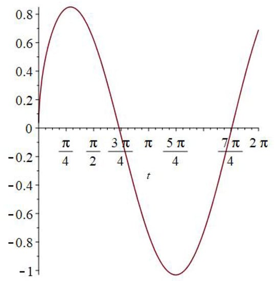
For ease of explanation, we choose $\alpha =\frac{1}{2}$, see also Figure 2. It holds that

$$\begin{array}{cc}\hfill {\displaystyle \left(D^{\frac{1}{2}}{v}^{\prime }\right)\left(t\right)}& {\displaystyle =t^{\frac{1}{2}}{E}_{2,\frac{3}{2}}(-t^2)}\hfill \\ & {\displaystyle =\sqrt{2}\left[cos\left(t\right)C\left(\sqrt{\frac{2t}{\pi }}\right)+sin\left(t\right)S\left(\sqrt{\frac{2t}{\pi }}\right)\right],}\hfill \end{array}$$

where the symbols C and S denote the Fresnel integrals [33] page 300

$$C\left(x\right)={\int }_0^{x}cos\left(\frac{\pi t^2}{2}\right)\mathrm{d}t,S\left(x\right)={\int }_0^{x}sin\left(\frac{\pi t^2}{2}\right)\mathrm{d}t.$$

Thus, we have

$$h\left(t\right)=sin\left(t\right)+\lambda (1-cos\left(t\right))+\sqrt{2}\left[cos\left(t\right)C\left(\sqrt{\frac{2t}{\pi }}\right)+sin\left(t\right)S\left(\sqrt{\frac{2t}{\pi }}\right)\right]$$

and

$$h^{\prime }\left(t\right)=cos\left(t\right)+\lambda sin\left(t\right)+\sqrt{2}\left(cos\left(t\right)S\left(\sqrt{\frac{2t}{\pi }}\right)-sin\left(t\right)C\left(\sqrt{\frac{2t}{\pi }}\right)\right)+\frac{1}{\sqrt{\pi t}}.$$

It holds (for any choice of λ)

$$h\left(0\right)=0,h^{\prime }\left(0\right)=\underset{t\to 0_{+}}{lim}{h}^{\prime }\left(t\right)=\underset{t\to 0_{+}}{lim}\left(1+\frac{1}{\sqrt{\pi t}}\right)=\infty ,h\left(2\pi \right)=\sqrt{2}C\left(2\right)>0.$$

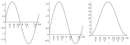
The only left free parameter to tune is λ. Please note that $h\left(t\right)$ consists of two parts. The first one is independent of λ – cf. Figure 3 (left). The second part is $\lambda (1-cos(t\left)\right)\ge 0$. Choosing sufficiently large $\lambda >0$, we can force $h\left(t\right)$ to be non-negative, see Figure 3.

Wrapping up, the ISP for determination of missing $f\left(\mathbf{x}\right)$ from the final time observation admits in addition to the trivial solution $\left(T\right(\mathbf{x},t),f(\mathbf{x}\left)\right)=(0,0)$ also a non-trivial one

$$(T(\mathbf{x},t),f\left(\mathbf{x}\right))=\left((1-cos(t\left)\right)e\left(\mathbf{x}\right),e\left(\mathbf{x}\right)\right),$$

where $-\Delta e=\lambda e$ with sufficiently large eigenvalue $\lambda >0$. Moreover, we see that $0\not\equiv h\left(t\right)\ge 0$ and the derivative $h^{\prime }\left(t\right)$ changes its sign. Therefore, we conclude that positivity of $h\left(t\right)$ is not sufficient to prove the uniqueness to the ISP (32).

Please note that, if $h^{\prime }\left(t\right)\ge 0$, then we would have uniqueness by Theorem 1.

5. Conclusions

We studied some fractional versions of the Dual-Phase-Lag equation arising in heat conduction processes. The source term was supposed to be in a separated form $h\left(t\right)f\left(\mathbf{x}\right)$. We considered an inverse source problem of recovery a solely space dependent source term $f\left(\mathbf{x}\right)$ from the final time observation. We showed uniqueness of a solution to this ISP for a general fractional Jeffrey-type model assuming $h\left(t\right)>0,h^{\prime }\left(t\right)\ge 0$, see Theorem 1. Assuming ${\tau }_T>{\tau }_q$, the assumptions in Theorem 1 can be relaxed to $0\not\equiv h\ge 0$, see Theorem 2. Remark 3 shows that, if ${\tau }_q>{\tau }_T$, which corresponds to a fractional Cattaneo–Vernotte model, the positivity of $h\left(t\right)$ cannot guarantee the uniqueness of a solution to the ISP.

References

- Cattaneo, C. A Form of Heat-Conduction Equations Which Eliminates the Paradox of Instantaneous Propagation. Compt. Rendus 1958, 247, 431. [Google Scholar]
- Vernotte, P. Les paradoxes de la theorie continue de l’equation de la chaleur. Compt. Rendus 1958, 246, 3154–3155. [Google Scholar]
- Tzou, D.Y. A Unified Field Approach for Heat Conduction From Macro- to Micro-Scales. J. Heat Transf. 1995, 117, 8–16. [Google Scholar] [CrossRef]
- Quintanilla, R. A condition on the delay parameters in the one-dimensional dual-phase-lag thermoelastic theory. J. Therm. Stress. 2003, 26, 713–721. [Google Scholar] [CrossRef]
- Xu, H.Y.; Jiang, X.Y. Time fractional dual-phase-lag heat conduction equation. Chin. Phys. 2015, 24, 034401. [Google Scholar] [CrossRef]
- Podlubný, I. Fractional Differential Equations: An Introduction to Fractional Derivatives, Fractional Differential Equations, to Methods of Their Solution and Some of Their Applications; Mathematics in Science and Engineering; Elsevier Science: Amsterdam, The Netherlands, 1998. [Google Scholar]
- Nohel, J.; Shea, D. Frequency domain methods for Volterra equations. Adv. Math. 1976, 22, 278–304. [Google Scholar] [CrossRef]
- Singh, J.; Gupta, P.K.; Rai, K. Solution of fractional bioheat equations by finite difference method and HPM. Math. Comput. Model. 2011, 54, 2316–2325. [Google Scholar] [CrossRef]
- Kumar, D.; Rai, K. Numerical simulation of time fractional dual-phase-lag model of heat transfer within skin tissue during thermal therapy. J. Therm. Biol. 2017, 67, 49–58. [Google Scholar] [CrossRef]
- Tzou, D. Macro- To Micro-Scale Heat Transfer: The Lagging Behavior; Chemical and Mechanical Engineering Series; Taylor & Francis: New York, NY, USA, 1996. [Google Scholar]
- Nassar, R.; Dai, W. Modelling of Microfabrication Systems; Microtechnology and MEMS; Springer: Berlin, Germany, 2003. [Google Scholar]
- Gajewski, H.; Gröger, K.; Zacharias, K. Nichtlineare Operatorgleichungen und Operatordifferentialgleichungen; Mathematische Lehrbücher und Monographien. II. Abteilung. Band 38; Akademie-Verlag: Berlin, Germany, 1974. [Google Scholar]
- Slodička, M. An investigation of convergence and error estimate of approximate solution for a quasilinear parabolic integrodifferential equation. Apl. Mat. 1990, 35, 16–27. [Google Scholar]
- Slodička, M. On the Rothe-Galerkin method for a class of parabolic integrodifferential problems. Mat. Model. 1991, 3, 12–25. [Google Scholar]
- Slodička, M. Application of Rothe’s method to evolution integrodifferential systems. Comment. Math. Univ. Carol. 1989, 30, 57–70. [Google Scholar]
- Slodička, M. Smoothing effect and regularity for evolution integrodifferential systems. Comment. Math. Univ. Carol. 1989, 30, 303–316. [Google Scholar]
- Grimmonprez, M.; Slodička, M. Full discretization of a nonlinear parabolic problem containing Volterra operators and an unknown Dirichlet boundary condition. Numer. Methods Partial Differ. Equ. 2015, 31, 1444–1460. [Google Scholar] [CrossRef]
- Khoa, V.A.; Dao, M.K. Convergence analysis of a variational quasi-reversibility approach for an inverse hyperbolic heat conduction problem. arXiv 2020, arXiv:2002.08573. [Google Scholar]
- Tuan, N.H.; Nguyen, D.V.; Au, V.V.; Lesnic, D. Recovering the initial distribution for strongly damped wave equation. Appl. Math. Lett. 2017, 73, 69–77. [Google Scholar] [CrossRef]
- Rukolaine, S.A. Unphysical effects of the dual-phase-lag model of heat conduction: Higher-order approximations. Int. J. Therm. Sci. 2017, 113, 83–88. [Google Scholar] [CrossRef]
- Rukolaine, S.A. Unphysical effects of the dual-phase-lag model of heat conduction. Int. J. Heat Mass Transf. 2014, 78, 58–63. [Google Scholar] [CrossRef]
- Liu, Z.; Quintanilla, R.; Wang, Y. On the regularity and stability of the dual-phase-lag equation. Appl. Math. Lett. 2020, 100, 106038. [Google Scholar] [CrossRef]
- Slodička, M.; Šišková, K.; Bockstal, K.V. Uniqueness for an inverse source problem of determining a space dependent source in a time-fractional diffusion equation. Appl. Math. Lett. 2019, 91, 15–21. [Google Scholar] [CrossRef]
- Luchko, Y. Maximum Principle and Its Application for the Time-Fractional Diffusion Equations. Fract. Calc. Appl. Anal. 2011, 14, 110–124. [Google Scholar] [CrossRef]
- Luchko, Y. Maximum principle for the generalized time-fractional diffusion equation. J. Math. Anal. Appl. 2009, 351, 218–223. [Google Scholar] [CrossRef]
- Mclean, W. Regularity of solutions to a time-fractional diffusion equation. ANZIAM J. 2010, 52, 123–138. [Google Scholar] [CrossRef]
- Stynes, M. Too much regularity may force too much uniqueness. Fract. Calc. Appl. Anal. 2016, 9, 1554–1562. [Google Scholar] [CrossRef]
- Duan, J.S.; Chen, L. Solution of Fractional Differential Equation Systems and Computation of Matrix Mittag–Leffler Functions. Symmetry 2018, 10, 503. [Google Scholar] [CrossRef]
- Sakamoto, K.; Yamamoto, M. Initial value/boundary value problems for fractional diffusion-wave equations and applications to some inverse problems. J. Math. Anal. Appl. 2011, 382, 426–447. [Google Scholar] [CrossRef]
- Schneider, W.R. Completely monotone generalized Mittag-Leffler functions. Expo. Math. 1996, 14, 3–16. [Google Scholar]
- Miller, K.S.; Samko, S.G. A note on the complete monotonicity of the generalized Mittag-Leffler function. Real Anal. Exch. 1999, 23, 753–756. [Google Scholar] [CrossRef]
- Garrappa, R.; Kaslik, E.; Popolizio, M. Evaluation of Fractional Integrals and Derivatives of Elementary Functions: Overview and Tutorial. Mathematics 2019, 7, 407. [Google Scholar] [CrossRef]
- Abramowitz, M.; Stegun, I.A. Handbook of Mathematical Functions with Formulas, Graphs, and Mathematical Tables, 10th ed.; Dover: New York, NY, USA, 1964. [Google Scholar]
© 2020 by the authors. Licensee MDPI, Basel, Switzerland. This article is an open access article distributed under the terms and conditions of the Creative Commons Attribution (CC BY) license (http://creativecommons.org/licenses/by/4.0/).