The Optimal Setting of A/B Exam Papers without Item Pools: A Hybrid Approach of IRT and BGP

Abstract

The administration of A/B exams usually involves the use of items. Issues arise when the pre-establishment of a question bank is necessary and the inconsistency in the knowledge points to be tested (in the two exams) reduces the exams ‘fairness’. These are critical for a large multi-teacher course wherein the teachers are changed such that the course and examination content are altered every few years. However, a fair test with randomly participating students should still be a guaranteed subject with no item pool. Through data-driven decision-making, this study collected data related to a term test for a compulsory general course for empirical assessments, pre-processed the data and used item response theory to statistically estimate the difficulty, discrimination and lower asymptotic for each item in the two exam papers. Binary goal programing was finally used to analyze and balance the fairness of A/B exams without an item pool. As a result, pairs of associated questions in the two exam papers were optimized in terms of their overall balance in three dimensions (as the goals) through the paired exchanges of items. These exam papers guarantee their consistency (in the tested knowledge points) and also ensure the fairness of the term test (a key psychological factor that motivates continued studies). Such an application is novel as the teacher(s) did not have a pre-set question bank and could formulate the fairest strategy for the A/B exam papers. The model can be employed to address similar teaching practice issues.

1. Introduction

1.1. Background

Resource-related conflicts may occur during term tests evaluating learning results and conducted among course participants within available classroom space. This may result in the infeasibility of unified exams (i.e., the use of the same exam papers at the same time). A common strategy used in this case is the random distribution of exams to students at different times. To address the disadvantages of administering exams across sessions, different exam papers must be administered for each exam session. When an exam is conducted in two sessions and requires two exam papers, an ‘A/B exam papers’ strategy is applied. Each exam paper normally has the same number of question items and contains items that consistently test the same set of various knowledge points.

Although the ‘A/B exam papers’ strategy aims for fairness between the two sessions, it has been observed to be not entirely fair when introduced in teaching practice. This phenomenon can be explained by the fact that even though A and B exam papers’ items are developed according to the same knowledge points, the items are not identical, which leads to differences among them in three item-parametric dimensions: difficulty, discrimination and guessing. Difficulty refers to the parameter of an item that governs how the item behaves over the ability scale, that is, the level of ability at which 50% of the respondents choose the correct response, whereas discrimination refers to the parameter of an item determining the rate at which the likelihood of choosing a correct response changes for differing ability levels [1]. Meanwhile, guessing refers to a parameter of an item that will be further discussed in Section 1.2.3. Thus, fairness cannot be achieved for students randomly assigned to take A/B exams. Such unfairness, accumulated through several pairs of items, leads to unpredictable and even more substantial testing unfairness (motivation).

To address this issue under the premise that the teacher does not need to pre-establish a question bank, the principle lies in the pair-wise exchange of items in A/B exam papers that test the same knowledge point, so the item sets necessary for both exam papers could be determined to maximize the fairness of the A and B exam papers overall in the three dimensions. Hence, the objective of this study was to develop a feasible model to adapt to such needs, so the model can provide all students with the opportunity to participate in a fairer (or nearly fair) exam effectively. As shown in the literature review, such a research question (RQ) is novel (objective).

For the methods, this study followed the recent data-driven decision-making (DDDM) concept [2]. With regards to data analytics and decision supporting, this study proposed the use of a hybrid model that combined item response theory (IRT) used in statistics and binary goal programing (BGP) used in operational research [3]. IRT was used to estimate the item parameters (with respect to (wrt) the three dimensions) for each question in the A and B exam papers in their original settings. Another BGP model that could suggest ‘exchange actions’ for item pairs was established. Finally, question sets were determined for the reproduced A’ and B’ exam papers so that examination fairness was ensured in their similarity in these dimensions. The resulting hybrid model was novel in terms of methodology.

Regarding data collection and data pre-processing, data were collected from the term test of a compulsory general course of multiple equally-taught classes, wherein exam participants came from multiple institutes. The most salient feature of this course was that the term test required the use of an ‘A/B exam papers’ strategy, but no item pool was available. In addition, several techniques were also applied during data pre-processing. Section 2 (Methods) gives a detailed description.

1.2. Literature Review

The literature study emphasized the implications of the exam fairness issue for educational psychology and the novelty of the RQ (absence of related systematic research), the relevance of the IRT model wrt the RQ, the relevance of the BGP model and the novelty of the combined IRT and BGP approach. First, the importance of the RQ is addressed.

1.2.1. Importance of the RQ

Issues regarding an effective test were addressed wrt test reliability and test practicality two decades ago [4]. However, how do we know if a test is reliable and practical? The influencing factors can be reviewed in a broader sense.

For practicality, an effective test is practical if it has the following attributes: (P1) it is not excessively expensive; (P2) it takes an appropriate length of time; (P3) it is easy to administer; and (P4) it utilizes a scoring/evaluation procedure that is efficient in terms of time while also being specific.

For reliability, a test is reliable if it is both consistent and dependable. The reliability of a given test can best be ensured if various factors that could make the test unreliable are taken into account and appropriately addressed. In other words, a reliable test is one that is fair to everyone, which entails both (R1) reliability for students and (R2) reliability for test administrators.

From the summary, resolving the RQ (to test with the A/B exam papers ‘effectively’ without the use of an item pool) is critical in practice because this exam papers setting strategy reduces the cost (P1) to maintain any item pool and the computerized solution allows simple test administration (P3), while the length of time and the efficiency of the evaluation procedure do not increase and the test remains ‘being specific’ (P4).

Resolving this RQ (to test with the A/B exam papers ‘fairly’ but still keeping the tested knowledge points consistent) is also critical because exam fairness is a psychological issue. The reliability for students (R1), certainly can be ensured by assigning who will participate in the exams using the reproduced A’ and B’ exam papers that are fairer randomly, while the size of the sample is usually sufficient to have two statistically even distributions for fairness. However, ensuring the reliability for test administrators (R2) usually involves setting two individual exam papers fairly because this can control the unreliable factors to an extent, but this often troubles the teacher.

1.2.2. Implications of Exam Fairness and Novelty of the RQ

Based on the preceding discussion, in the present study, the term ‘fairness’, although difficult to define, is essentially used to refer to the fairness of a test (that is, as opposed to other issues of fairness, such as fairness in scheduling [5], that is, the degree to which any differences in the three item-parametric dimension between two different tests are eliminated. Fairness, which is an essential aspect of a test, refers broadly to the equitable treatment, over the course of the testing process, of all the individuals taking a test, which includes unbiased access to the measured constructs, no measurement bias, and clear validity in the interpretation of test scores for the proposed purpose(s). That said, a clear definition of the word fairness is difficult to produce, insofar as the primary concept of testing fairness is, as expressed in The Standards for Educational and Psychological Testing, ‘to identify and remove construct-irrelevant barriers to maximal performance for any examinee’ [6]. Relatedly, in the event that test scores used for the purposes of assessment differ substantially in terms of, for example, racial groups, there is some potential that associated decisions pertaining to members of lower scoring groups may be unfair. As such, fairness can be defined as the removal of any systematic variation resulting from racial or cultural socialization experiences from test scores, and it is therefore distinct from cultural bias and test-score validity [7]. Relatedly, the various meanings of ‘fairness’ in assessment were also extensively discussed in a study by Camilli [8]. The fairness of a test is an extremely important ethical issue, from educational and psychological perspectives, for both teachers and students. This issue was once defined by Shohamy [9], who stated that tests are essentially a form of social technology that plays a central role in education, business, and government, with tests frequently being the sole factors in deciding the futures of test-takers. As such the people who design testes should feel an obligation to meet and uphold the specific standards set by the educational institutions that they serve.

Relatedly, the ethics of testing are a form of what educators term critical pedagogy, but standardized testing on a large scale is not a process without bias. Rather, it is affected by various aspects of society, culture, and politics, as well as by specific ideological and educational agendas, that mold the lives of all those who take part in the process, including students, teachers, and others [10]. Therefore, the design and administration of a large-scale standardized test [11,12] involve the issue of fairness for the different groups of participants [13].

As A/B exam papers are an important means of ensuring fairness, setting (and ‘aligning’) them consistently and fairly takes care of group interests of both students (e.g., positive course experience for continued learning) and teachers (e.g., reducing negative feedbacks, mitigate the effects that any member in the teaching roster is lack of personal understanding about educational assessment, etc.) [14,15,16,17,18]. However, the question of exactly how best to achieve fairness remains for setting the A/B exam papers without an item pool. In the literature, studies addressing such a RQ would be few (see further discussions in Section 1.2.3).

1.2.3. Relevance of the IRT wrt the Analysis of the RQ

Lord proposed a two parameters normal ogive model, which is considered to be the origin of IRT (or latent trait theory) [19]. In later years, psychologists developed an IRT model with three parameters [20], the generalized form of which will be presented in the methods section. It has long been known by psychometricians that guessing constitutes a substantial threat to test score validity and that it can, relatedly, be a cause of construct irrelevant variance. There are a several ways in which guessing behaviors are typically investigated, but almost all of these methods of investigation entail the administration of a test to an appropriate sample and then analyzing the resulting response patterns and scores for any indications that guessing may have taken place. To that end, we chose to create a test consisting of items actually relevant to medical school courses and then to administer that test to university staff members of a medical education administrative office. Because none of these administrative staff members actually had any formal experiences or education in the fields of medicine or health sciences, we theorized that they would be forced to rely almost completely on guessing strategies when taking the exam. In other words, by intentionally having an inappropriate sample take the exam, we were able to investigate guessing in a more deliberate manner, better determine the ways in which guessing might affect the test scores of our medical students, and better identify the specific exam items that appeared to be vulnerable to test wise-ness. With respect to fairness, the key questions in this regard are whether or not the social consequences of an exam and/or the associated examination practices can contribute to societal equity and whether or not a particular exam or examination program has any pernicious effects. Relatedly, it has been suggested by Griffore [21] that avoiding the use of valid tests that have been called unfair due to culturally or racially based construct-irrelevant variance is itself unfair if those tests can, in fact, assist individuals in making decisions that ultimately result in successful outcomes.

Since its proposition, IRT has been widely applied. Both social and education sciences give high consideration to the issue of civic scientific literacy (CSL). In the 1990s, Miller estimated the item question parameters of a CSL questionnaire and applied IRT to calculate individual and group ‘CSL latent levels’ for the understanding of scientific concepts, thus replacing the correct answering rate (CAR) measure used to calculate total scores directly based on answers. As a result, a so-called ‘3D measure’ was established [22], which was later followed in CSL studies conducted in different countries, including Europe, Japan, South Asia and Central and South America [23,24,25,26,27]. Starting from this century, because of the implementation of IRT in that field, cross-country comparisons have been based on an objective foundation rather than subjective scoring [28,29]. These observations have strengthened our confidence in using IRT.

With regard to the question setting issue in Education, Lord [30] proposed the following four steps for the compilation of an exam paper using test information function:

• Decide on the desirable curve and target for the information function, based on the testing objective.
• Select a set of items from a question bank and calculate the test information amount for each item.
• Add and delete items and recalculate the sum of information amounts for all included items.
• Repeat steps 2–3 until the aggregated information amount approaches the target for the test and becomes satisfactory.

This IRT-based method is supported by a statistical foundation. However, empirical studies have discovered that the compiled paper often lacks content validity (see Appendix A). Therefore, Yen [31] proposed computerized item choice and paper compilation as means to address issues related to the manual compilation and complex processing used in the case of a large number of available items; the scholar integrated linear programing (LP) modelling. Later studies by Theunissen [32], Boekkooi-Timminga [33], Boekkooi-Timminga and van der Linden [34] also used binary programing (BP) modelling to compile papers for different exams. Adema [35] and Swanson and Stocking [36] used BP modelling to compile questions for parallel tests. However, these subsequent studies were initially aimed at automating the test compilation process following the estimation of item parameters using IRT.

Thus, according to this review, first, IRT was proposed as a theory for psychological statistics but, in addition to use in other fields (e.g., CSL), has been widely used in exam paper compilation in Education. This describes the relevance of the IRT model for this study.

Next, the related studies discussed above involved the pre-establishment of a large question bank. The questions selected from which were used to compile one single (or several single ones individually) exam paper to meet the target and maintain balance in each dimension. Nevertheless, under different circumstances (e.g., the studied case), teachers often cannot pre-establish any such question bank in teaching practice. They design test items based on the knowledge points they want to test according to the teaching content for a certain period of time, in particular, in the cases of ‘course dynamics’ (i.e., a new teacher every semester), large numbers of teaching participants and the joint design of test items. In fact, the authors have found no study that discussed the balance and fairness of A/B exam papers in the absence of a question bank. This is the greatest difference between this study and other studies.

Finally, as many relevant studies used mathematical programing (MP) (e.g., LP or BP) after the use of IRT, they confirmed the feasibility of this study’s model integration (i.e., using BGP after IRT). However, the use of BGP is a must in this study because of the abovementioned ‘great difference’.

1.2.4. Relevance of BGP and the Novelty of the IRT–BGP Approach

Goal programing (GP) was proposed by Charnes and Cooper [37]. GP modelling is also another MP approach that deals with multiple explicit goals in the decision context and allows the decision-maker to consider these goals simultaneously [38]. Thus, it is now a key approach in the multi-objective programing (MOP) field [39,40,41,42,43]. In addition, it is also a flexible decision analysis tool when the problem involves conflicting goals subject to a number of complex decision constraints [44,45,46]. Therefore, there are also a great number of studies that use GP to support the various decision-analysis demands in actual practice, e.g., healthcare, agriculture, economics, engineering, transportation and marketing [47,48,49,50,51,52,53].

GP also supports the decision of discrete optimization. In the field of GP, the mixed-integer GP (MIGP) modelling approach is a special case of GP where any solution vector in the feasible solution set contains only integer elements, whilst the BGP modelling approach is a special case of the MIGP where the vector contains only 0–1 binary variables.

Using BGP is appropriate because it meets the purpose of this study, as the problem to be solved is: how the paired questions produced to test the same knowledge, one per version of the exam paper, should be exchanged so as to achieve the fairness objectives in the three dimensions. Therefore, the matter to be decided is ‘whether each pair of two such questions should be exchanged or not’, which can be connoted by a 0–1 variable. The 0–1 variables for all pairs determine an ‘exchange plan’ over two exam papers, rather than any suitable ‘organization’ of each exam paper. It is, intrinsically, a discrete optimization problem which is only solvable by BGP.

Therefore, unlike the studies wherein hybrid test compilation methods such as IRT–LP or IRT–BP are used, the IRT–BGP model is developed. Despite the different purposes of these models, the application of IRT–BGP on test compilation, however, is novel.

1.3. Results: A Brief

The topic of interest is the item exchange between A/B exam papers to achieve exam fairness. The research results have certain implications from the perspective of educational psychology research. The content of A/B exam papers after item exchange (i.e., A’ and B’ exam papers) is fair from the students’ perspective (for example, classmates assigned to take different exam papers are less likely to argue about the exam results). This is also beneficial for teachers in teaching practice, the main benefits being that fairer exam papers can be obtained for actual large-scale testing and a pre-set question bank is not needed when many teachers participate in the teaching and development of a large course and are changed each year, thus leading to changes in course and examination content.

Section 2 introduces the methods. Section 3 presents the main results. A descriptive analysis is presented to carry out observations of the extent of unfairness in the original A/B papers, followed by estimating the item parameters using IRT and achieving the fairness of the two papers using BGP. Section 4 conducts several extensive analyses in order to explore the relevant implications. A process for future application of the approach is also suggested. The last section provides the conclusion.

2. Methods

2.1. Experimental Flow

Figure 1 shows the flowchart for this study. It is designed in accordance with the standard process for DDDM; Appendix B offers extensive discussions.

For data collection, the researchers collected data concerning detailed answers and the performance scores (based on the traditional CAR justification) of students who were allocated randomly to take the A and B exam papers in a term test. The exams were administered for a compulsory general course teaching basic computer programing techniques. In total, 298 first-year university students from 11 colleges took this course during the fall semester studied. Because of the lack of classroom resources in the school, the course was taught equally in 6 classes (i.e., the same topic was taught by the same teacher in each class). Students needed to be divided not only for studies but also for tests. As the university had no auditorium that could hold them, the ‘A/B exam papers’ strategy is necessary to use for the term test. The exams were conducted in two sessions which used the A exam paper (149 students) and B exam paper (149 students), respectively. The course teacher group designed 20 multi-choice question items for each exam paper based on the course content taught. The items paired under the same item number were associated in terms of the terminology.

After the exam, the researchers applied to the exam paper storage center (the committee on general core courses in the university) and were authorized to “borrow and record exam paper answers under the prerequisite of de-identification.” The center also provided the ‘standard answers,’ that is, the correct answers for the 20 items in each exam paper. As such, raw data were collected.

For data pre-processing, together with the CAR scores available for each student, an item-by-item inspection for each exam paper returned was conducted to code the students’ correct and incorrect answers as 1 and 0, respectively. These were registered in an Excel file. Pivot analysis was performed to test for abnormal values and data irrationalities. The scores of the only one student who did not answer any question in the B exam paper were eliminated according to the complete case study method commonly used in medicine to keep the data faithful. All results were saved into a data warehouse for the latter data analysis and decision-making/supporting phases.

2.2. IRT Modelling

The data analysis phase uses IRT. The general ‘IRT 3PL model’ can be used to introduce general IRT principles because in this study, all items are multiple-choice questions as the testing items in the CSL survey. Miller (1998) presented the 3PL IRT model, as:

$$T({\theta }_r;{\mathsf{\Psi }}_j)=c_j+\frac{1-c_j}{1+e^{-a_j({\theta }_r-b_j)}}$$

(1)

where ${\mathsf{\Psi }}_j=\{a_j,b_j,c_j\}$ is a parameter set for the j-th test question item; a_j, b_j and c_j are, respectively, the discrimination, difficulty and lower asymptotic parameter (or guessing, that is, the CAR baseline) of the question; ${\theta }_r$ is the latent variable connoting the r-th respondent’s level of ability.

This formula was to measure a set of parameters ${\mathsf{\Psi }}_j$ for each question item j in an exam paper based on statistical estimations, as well as the latent ability of each respondent r. The values in ${\mathsf{\Psi }}_j$ were the basis for the pairwise exchange of items in the later phase using the BGP model. Theoretically, for each a_j, b_j and c_j in ${\mathsf{\Psi }}_j$, −∞ < a_j < +∞, −∞ < b_j < +∞ and 0 ≤ c_j ≤ 1 [54].

2.3. BGP Modelling

Following from Section 1.2, there is no existing model which can be referenced for the studied problem. So, this study uses BGP as the approach to make an ‘exchange plan’ for how the paired testing items in the two exam papers should be exchanged subject to the fairness requirements.

In order to balance the exam papers to pursue fairness, a model for exchanging the testing items in the A and B exam papers wrt the three criteria (in three dimensions) is constructed according to the standard form of a BGP model in Appendix C, as the following:

(BGP–IEP (item exchange planning))

$$Min{\displaystyle \sum _{i\in PL}{w}_i(d_i)}$$

(2)

s.t.

$$S_i^{A^{\prime }}={\displaystyle \sum _{j\in \{1,\dots ,N\}}\left(p_{ji}^A{y}_j+p_{ji}^B(1-y_j)\right)},\forall i\in PL$$

(3)

$$S_i^{B^{\prime }}={\displaystyle \sum _{j\in \{1,\dots ,N\}}\left(p_{ji}^A(1-y_j)+p_{ji}^B{y}_j\right)},\forall i\in PL$$

(4)

$$\left|S_i^{A^{\prime }}-S_i^{B^{\prime }}\right|-d_i=0,\forall i\in PL$$

(5)

$$y_j\in \{0,1\},j=\{1,\dots ,J\}$$

(6)

$$d_i\ge 0,\forall i\in PL$$

(7)

where PL is the set of question parameters considered as the criteria to balance the exam papers; y_j is the binary decision variable controlling whether the j-th pair of associated questions should be exchanged; define E ϵ {A, B} (A and B are the original exam papers), $p_{ji}^E$ is the i-th item parameter as estimated from the analysis of IRT for the j-th question in an original exam paper E; define E’ ϵ {A’, B’} (A’ and B’ are the new exam papers), $S_i^{E^{\prime }}\in R$ is the gap that remains between the two new exam papers in E’ for the i-th item parameter, after the exchanges; and N is the number of questions in each exam paper; $d_i$ and $w_i$ are, respectively, the surplus (or positive) deviational variable and the test administrator’s preferential weight toward the i-th goal criterion (parameter), relative to other criteria.

In this model, PL = {discrimination, difficulty, guessing} means that it is able to suggest the exchanges by balancing every item parameter that are assessed by the 3PL model of IRT. However, if PL = {discrimination, difficulty}, then only the discriminative power and the difficulty of the two exam papers are balanced. Thus, this flexible model can be generalized as per the test administrator’s wish.

For this model, the solution, the one-dimensional binary vector, Y*, determines an ‘exchange plan’. It details which pairs of associated questions in the two original exam papers should be exchanged (i.e., the individual y_j* values 1 indicates that the j-th pair should be exchanged) and which pairs should not (i.e., y_j* = 0) to constitute the new A’ and B’ exam papers. In other words, it is not used to determine whether a question in the existing item pool should be included or not, as in previous IRT–BP studies.

In the above (BGP–item exchange planning) model, the goals are to minimize the unidirectional absolute distance between two exam papers in each goal criterion (see Equation (5)). Thus, it is straightforward to formulate only a surplus variable, $d_i$, for each item-parametric dimension that is considered, i.e., i ϵ PL. However, the test administrator(s) would sometimes like to gain information ‘with directions’ about how each of the goals are optimized, i.e., whether a positive deviation or a negative deviation between the new exam papers A’ and B’ still exists? In this case, Equation (5) is further linearized, and both surplus and slack variables can be introduced (see also (Martel and Aouni, 1990)). This gives Equations (9), with a new Equation (10) and a new objective function, which is Equation (8):

$$Min{\displaystyle \sum _{i\in PL}{w}_i(d_i^{+}+d_i^{-})}$$

(8)

$$\left(S_i^{A^{\prime }}-S_i^{B^{\prime }}\right)-d_i^{+}+d_i^{-}=0,\forall i\in PL$$

(9)

$$d_i^{+}\ge 0,d_i^{-}\ge 0,\forall i\in PL$$

(10)

Substituting the above Equation (5) in the (BGP–item exchange planning) model with Equation (9) and using Equation (8) and Equation (10) as the replacements for Equation (2) and Equation (7) yields another new model, which can be called the (BGP–IEP II) model. The fully linearized model can be written and solved by almost all LP packages without extension functional supports for absolute values (e.g., in LINGO).

Moreover, in either Equation (2) or Equation (8), the weight-additive GP variant is applied [55,56]. This adheres to the principle of simplicity in proposing a scientific concept (i.e., the problem-model fitting for this study) [57]. As the incommensurability of the various objectives may create problems [58], the gaps measured by these models between two exam papers (i.e., $\left|S_i^{A^{\prime }}-S_i^{B^{\prime }}\right|$ or $\left(S_i^{A^{\prime }}-S_i^{B^{\prime }}\right)$) can be further aggregated to be commensurable. Although the distance from one exam paper to another (i.e., $d_i$ or the term ($-d_i^{+}+d_i^{-}$)) in each dimension is purely numerical without any unit (because the parameters in Equations (3) and (4) are all numerical), which is unlike the objectives possessing incommensurable measurement units, similar rules can be applied. In this sense, additional intervals can be introduced to normalize the distance or deviation for each objective. Suppose that ${\Delta }_i$ connotes the ‘suitable range’ for the i-th item parametric dimension in the studied problem, the normalized expression to aggregate the objectives becomes:

$$Min{\displaystyle \sum _{i\in PL}{w}_i(\frac{d_i}{{\Delta }_i})}\mathrm{for}(\text{BGP–IEP}),\mathrm{or}Min{\displaystyle \sum _{i\in PL}{w}_i\frac{(d_i^{+}+d_i^{-})}{{\Delta }_i}}\mathrm{for}(\text{BGP–IEP II})\mathrm{alternatively}.$$

(11)

Note that although the bounds and some ‘usually seen ranges’ of the parameters assessed by IRT are suggested (see also Section 2.2), they are often contextually dependent, so that the ‘suitable range’ (${\Delta }_i$) should vary on a case-by-case basis.

Lastly, another model enhancement relates to the use of the min-max concept or the max-min concept [59,60]. For example, the objective function of (BGP–IEP II) (Equation (8)) could also be re-written semantically as the following, whilst one may refer to Romero [42] for the linearization process of the function in the GP context:

$$MinMax\left\{{\displaystyle \sum _{i\in PL}{w}_i{d}_i^{+}},{\displaystyle \sum _{i\in PL}{w}_i{d}_i^{-}}\right\}$$

(12)

2.4. Short Summary

The method used in previous studies of IRT-based exam paper compilation is detailed in Appendix D. Method-wise, regardless of whether any MP model was used for automating the process, an exam paper that could meet the information targets (required in the dimensions) to the greatest extent possible was designed. In the case, designing two fair A/B exam papers involved two rounds of the process with identical targets set. However, this required a question bank.

In contrast, this study is based on another common case when no question bank is available. While there is nothing to do with the innate parameters of the items in the given A/B exam papers, but the pursuit of a fair A/B test is still the concern, the fairness of two exam papers is sought for by carrying out pair-wise exchanges of items so as to achieve a balance in the three dimensions. The only commensurable property of these two approaches is the use of IRT.

Therefore, a systematized IRT–BGP approach is proposed. To the best of the authors’ knowledge, it has no analogues in current research, in terms of either model integration or modelling purpose. It is a different approach compared to those in previous studies that have also used the IRT. This makes it a novel and niche one.

3. Results

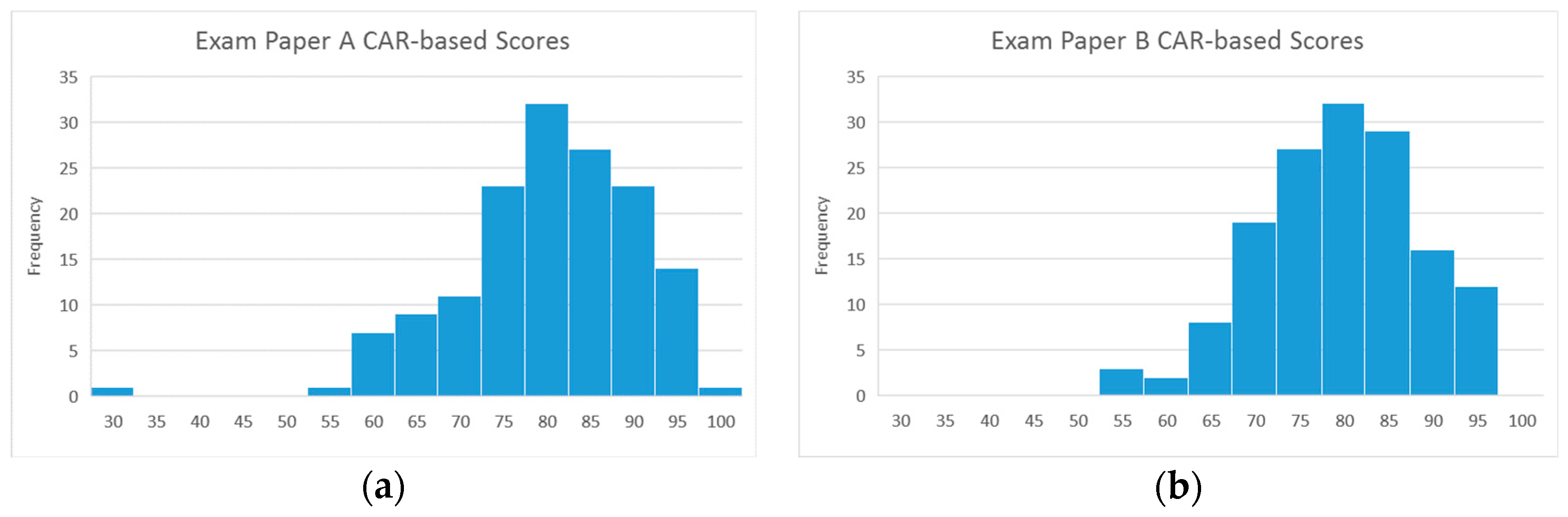
3.1. The Unfair A/B Test

The unfairness of the original A/B test is shown by a descriptive statistical analysis using students’ answers. As they were randomly assigned, it could be assumed that students with different abilities were evenly distributed to two participant groups. Under this premise, any difference in CAR would indicate the unfairness.

Table 1. The correct answering rate (CAR) to each question in A/B exam papers and the gaps.

Item	Q1	Q2	Q3	Q4	Q5	Q6	Q7	Q8	Q9	Q10
A	87.2%	87.9%	45.6%	100%	94.6%	62.4%	82.6%	98.0%	96.6%	22.8%
B	98.0%	93.9%	98.6%	54.7%	80.4%	76.4%	52.7%	95.9%	37.2%	97.3%
|A–B|	10.80%	6.00%	53.00%	45.30%	14.20%	14.00%	29.90%	2.10%	59.40%	74.50%
Item	Q11	Q12	Q13	Q14	Q15	Q16	Q17	Q18	Q19	Q20
A	55.0%	94.0%	99.3%	91.9%	75.2%	98.0%	98.0%	81.9%	38.3%	93.3%
B	92.6%	98.6%	85.1%	87.2%	51.4%	100%	96.6%	77.0%	29.1%	87.2%
|A–B|	37.60%	4.60%	14.20%	4.70%	23.80%	2.00%	1.40%	4.90%	9.20%	6.10%

demonstrates the CAR for each item for these two test-participant groups. As seen from the table, the difference in CAR exceeded 20% for seven item pairs (Q3, Q4, Q7, Q9, Q10, Q11 and Q15) using the two papers.

The distribution of CAR in Figure 2 also indicates substantial differences in students’ performance between the exam papers. All this indicated that the original A/B exam papers did not allow the two groups of students to be examined fairly, and thereby violated their rights severely.

3.2. Estimating the Item Parameters Using IRT

The IRT 3PL model was used to analyze the pre-processed data and estimate the three parameters for each item. These are summarized in

Table 2. The estimated item response theory (IRT) model parameters for all question items in the two exam papers.

	A Exam Paper			B Exam Paper
Qj	PjAguessing	PjADifficulty	PjADiscrimination	PjBguessing	PjBDifficulty	PjBDiscrimination
Q1	0.062693	−5.28596	0.35833	0.371513	−4.67323	0.788151
Q2	0.733727	−0.11029	4.477341	0.010156	−5.40925	0.525375
Q3	0.073052	0.524729	0.757966	0.036918	−4.31039	1.127738
Q4	0.999148	−16.0528	0.182542	1.8 × 10−14	−0.32322	0.616322
Q5	0.082952	105.6133	−0.0263	0.000153	−2.33305	0.655196
Q6	0.265127	0.05209	1.432473	1.1 × 10−17	−0.68727	31.1551
Q7	0.052179	−2.63839	0.605141	0.491215	−3.0337	−0.97887
Q8	0.057648	−2.40507	3.092044	0.908461	−0.14645	3.522721
Q9	0.07932	−5.7558	0.597789	0.000115	3.946901	0.134206
Q10	0.151572	2.907607	0.900514	0.067808	−42.2536	0.083154
Q11	0.343063	1.018947	0.886161	0.006117	4.488719	−0.59619
Q12	0.009758	−2.09139	1.962636	7.98 × 10−8	2.201958	−31.5338
Q13	0.06416	−4.66897	1.220194	2.52 × 10−6	4.233981	−0.4289
Q14	0.018908	−2.44744	1.211052	0.000189	−3.02158	0.687387
Q15	0.002061	−0.72737	3.737409	1.46 × 10−11	−0.12289	0.416349
Q16	0.052894	−4.75631	0.885629	1	18.33097	−0.4557
Q17	0.017352	−2.26877	4.149376	0.018236	3.143843	−1.31879
Q18	0.022078	−2.16509	0.759793	0.013546	−9.85322	0.121235
Q19	0.28291	1.288772	2.668051	0.261825	−1.85502	−6.41667
Q20	0.061449	−3.56639	0.791395	0.004878	13.74994	−0.13957
Total	3.43205	56.46538	30.64953	3.191133	−27.9266	−2.03558

.

The comparison of the estimated parameters also showed severe unfairness. All pairs of the associated items in the two original exam papers considerably differed in terms of their difficulty and discrimination, which corresponded to the differences in CAR discussed earlier. These illustrated that failure to apply a mechanism in the planning of A/B exam paper questions had violated the students’ rights severely and, consequently, damaged the school’s reputation.

Supporting evidence was also found in the item distribution: some unsuitable items were found and their appearance was also unbalanced. The left-hand figures in Figure 3a,b demonstrate the distribution of the difficulties and discriminations of the A/B exam paper questions. However, because of a number of outliers, using a normal scale cannot demonstrate the relations between the difficulty and discrimination of each item easily. The rank-rescaled distributions are therefore visualized in order to identify the attributes of any item (in Table 2) easily.

If an ‘absolute measure’ is used, then, in the figures, none of the items in the A paper but four items in the B paper (Q11, Q13, Q16, Q17) are characterized by high difficulty (difficulty > 2.5) and low discrimination (discrimination < −0.4) (see the lower right part). In contrast, the B paper contained four items (Q1, Q2, Q3, Q14) with low difficulty (difficulty < −2.5) and high discrimination (discrimination > 0.4), while the A paper contained more such questions (Q7, Q9, Q13, Q16, Q20). These are usually the ‘unsuitable questions’.

If another ‘relative measure’ is used, then, in the right-hand figures, two items in the A paper (Q3, Q5) but five items in B (Q11, Q12, Q13, Q16, Q17) are characterized by high difficulty (the rank in difficulty is ≥14, i.e., between 15 and 20) and low discrimination (the rank in discrimination is ≤7). In addition, the A paper contained no item with low difficulty (the rank in difficulty is ≤7) and high discrimination (the rank in discrimination is ≥14), but the B paper contained three such items (Q1, Q3, Q14). Both analyses have shown the imbalance in these unsuitable questions in the two exam papers.

3.3. Modelling the Problem Using the BGP Model

As establishing a question bank was infeasible for the A/B test of the course, using any previous item-pool-based model to compile two individual papers was infeasible. A model is constructed based on (BGP–item exchange planning) in 2.3 using real data. Let I = 3, PL be the set of {discrimination, difficulty, guessing} and J = 20 for the case studied. Let the values of the model parameters, $p_{ji}^A$ and $p_{ji}^B$, where j = 1…20 and i = 1…3, be the corresponding item parametric elements in Table 2. By limiting y_j (j = 1…20) as binary variables and manifesting that $w_i=1$ (i = 1…3), the model is solved. Because of non-linearity, the optimal binary vector, Y^*, is obtained after 9863 solver iterations with 1 extended solver step:

$$\begin{array}{ll}{Y}^{*}& =\left[y_1^{*},y_2^{*},y_3^{*},y_4^{*},y_5^{*},y_6^{*},y_7^{*},y_8^{*},y_9^{*},y_{10}^{*},y_{11}^{*},y_{12}^{*},y_{13}^{*},y_{14}^{*},y_{15}^{*},y_{16}^{*},y_{17}^{*},y_{18}^{*},y_{19}^{*},y_{20}^{*}\right]\\ & =\left[1,1,1,0,0,0,0,1,0,1,1,0,1,1,1,0,1,1,0,0\right]\end{array}$$

This vector suggests an ‘exchange plan’ for the paired questions in two original exam papers, which is shown in

Table 3. The exchanging plan according to the optimal decision vector obtained.

Question Items in Exam Paper A	Planned Exchanges	Question Items in Exam Paper B	Remark (yi)
Q1	⇋	Q1	1
Q2	⇋	Q2	1
Q3	⇋	Q3	1
Q4		Q4	0
Q5		Q5	0
Q6		Q6	0
Q7		Q7	0
Q8	⇋	Q8	1
Q9		Q9	0
Q10	⇋	Q10	1
Q11	⇋	Q11	1
Q12		Q12	0
Q13	⇋	Q13	1
Q14	⇋	Q14	1
Q15	⇋	Q15	1
Q16		Q16	0
Q17	⇋	Q17	1
Q18	⇋	Q18	1
Q19		Q19	0
Q20		Q20	0
Summary			11

.

According to Table 3, to form the new A’ and B’ exam papers, a total number of 11 item pairs in A and B should be exchanged, i.e., that the following set of questions in both exam papers A and B be exchanged while keeping the rest unchanged: {Q1, Q2, Q3, Q8, Q10, Q11, Q13, Q14, Q15, Q17, Q18}.

The model’s objective based on this ‘exchange plan’ reveals its effectiveness, which is as small as: ${\displaystyle \sum _{i\in PL=\left\{\mathrm{discrimination},\mathrm{difficulty},\mathrm{guessing}\right\}}{w}_i(d_i)}=0.7738291$.

Furthermore, this can be decomposed as:

$d_{\mathrm{discrimination}}^{+}=0.5587864$, $d_{\mathrm{difficulty}}^{+}=0.2008591$ and $d_{\mathrm{guessing}}^{+}=0.01418366$.

These are the gaps in the three dimensions that still exist between the new A’ and B’ papers and refer to the nearly ideal status after minimising the differences in total discriminative power, total difficulty and total guessing probability between the two tests. Note that in this model the absolute distance of the gap remaining in each dimension (i.e., on the LHS of Equation (5)) is always ≥0. Also see Appendix E for the tools used to implement the entire IRT–BGP model.

The above solution set is obtained using the (BGP–item exchange planning) model. Appendix F provides an extensive analysis using the (BGP–IEP II) model and some comparisons based on the two solution sets.

4. Discussion and Implications

4.1. Analysis of the Exchange Plan

At first, after the exchanges, the total discriminative power, the total difficulty, and the total guessing of each new exam paper (that is, those behind the minimized differences but which are used to determine the magnitude of them), $S_i^{E^{\prime }},E^{\prime }\in \{A^{\prime },B^{\prime }\},i\in PL$, can be further analyzed. The item parameters in these new papers are detailed in

Table 4. The detailed parameter values of the A’ and B’ exam papers after exchanging.

	Exam Paper A’			Exam Paper B’
Qj	pj(guessing)	pj(difficulty)	pj(discrimination)	pj(guessing)	pj(difficulty)	pj(discrimination)
Q1	0.371513	−4.67323	0.788151	0.062693	−5.28596	0.35833
Q2	0.010156	−5.40925	0.525375	0.733727	−0.11029	4.477341
Q3	0.036918	−4.31039	1.127738	0.073052	0.524729	0.757966
Q4	0.999148	−16.0528	0.182542	1.80 × 10−14	−0.32322	0.616322
Q5	0.082952	105.6133	−0.0263	0.000153	−2.33305	0.655196
Q6	0.265127	0.05209	1.432473	1.10 × 10−17	−0.68727	31.1551
Q7	0.052179	−2.63839	0.605141	0.491215	−3.0337	−0.97887
Q8	0.908461	−0.14645	3.522721	0.057648	−2.40507	3.092044
Q9	0.07932	−5.7558	0.597789	0.000115	3.946901	0.134206
Q10	0.067808	−42.2536	0.083154	0.151572	2.907607	0.900514
Q11	0.006117	4.488719	−0.59619	0.343063	1.018947	0.886161
Q12	0.009758	−2.09139	1.962636	7.98 × 10−8	2.201958	−31.5338
Q13	2.52 × 10−6	4.233981	−0.4289	0.06416	−4.66897	1.220194
Q14	0.000189	−3.02158	0.687387	0.018908	−2.44744	1.211052
Q15	1.46 × 10−11	−0.12289	0.416349	0.002061	−0.72737	3.737409
Q16	0.052894	−4.75631	0.885629	1	18.33097	−0.4557
Q17	0.018236	3.143843	−1.31879	0.017352	−2.26877	4.149376
Q18	0.013546	−9.85322	0.121235	0.022078	−2.16509	0.759793
Q19	0.28291	1.288772	2.668051	0.261825	−1.85502	−6.41667
Q20	0.061449	−3.56639	0.791395	0.004878	13.74994	−0.13957
Total	3.318683	14.16897	14.02758	3.3045	14.36983	14.58637

. A digest is presented in

Table 5. Effectiveness of the solution in comparison with that of the original exam paper settings.

Attributes of A’	Value	Gap	Attributes of B’	Value
$S\begin{array}{c}{A}^{\prime }\\ \mathrm{Discrimination}\end{array}$	14.58637	0.5587864	$S\begin{array}{c}{B}^{\prime }\\ \mathrm{Discrimination}\end{array}$	14.02758
$S\begin{array}{c}{A}^{\prime }\\ \mathrm{Difficulty}\end{array}$	14.36983	0.2008591	$S\begin{array}{c}{B}^{\prime }\\ \mathrm{Difficulty}\end{array}$	14.16897
$S\begin{array}{c}{A}^{\prime }\\ \mathrm{Guessing}\end{array}$	3.304500	0.01418366	$S\begin{array}{c}{B}^{\prime }\\ \mathrm{Guessing}\end{array}$	3.318683
Subtotal		0.7738291
Attributes of A	Value	Gap	Attributes of B	Value
$S\begin{array}{c}{A}^{\prime }\\ \mathrm{Discrimination}\end{array}$	30.64953	32.68511	$S\begin{array}{c}{B}^{\prime }\\ \mathrm{Discrimination}\end{array}$	−2.03558
$S\begin{array}{c}{A}^{\prime }\\ \mathrm{Difficulty}\end{array}$	56.46538	84.39198	$S\begin{array}{c}{B}^{\prime }\\ \mathrm{Difficulty}\end{array}$	−27.9266
$S\begin{array}{c}{A}^{\prime }\\ \mathrm{Guessing}\end{array}$	3.43205	0.240917	$S\begin{array}{c}{B}^{\prime }\\ \mathrm{Guessing}\end{array}$	3.191133
Subtotal		117.318007

, where these values are also compared to a digest regarding the corresponding values of the original exam papers A and B. Note that if the exchanging actions are not guided by the optimal solution set Y*, but rather by another set which is the 2′s complement of it, Y*’, so that a total number of 9 questions are exchanged and the set of exchanged question pairs in exam papers A and B is {Q4, Q5, Q6, Q7, Q9, Q12, Q16, Q19, Q20}, the content of Table 4 is flipped, i.e., the values on the right side are exchanged with those on the left side. However, this should not affect the post-decision actions because the two determined exam papers can be used interchangeably for the two defined testing time slots, as long as their settings are fair.

From Table 5, it is obvious that the accumulated gap in terms of the differences between A’s and B’s item parameters was 117.318007. The two original papers differed in discrimination power and guessing probability, but these are not as critical as the large difference present in the difficulty dimension, i.e., paper A was much harder. This reflects the fact that some students who participated in the test that used the A exam paper expressed doubts regarding the fairness of the test.

It is also obvious that the proposed model is effective because now the total gap between the new A’ and B’ papers is as small as 0.7738291, and the gap in every dimension has been reduced to less than 1. For the studied case, it is fortunate to have such an outcome because the maximum fairness of the exams (i.e., as measured by the extent to which the gap approaches 0) after one such homogenization process is highly dependent on the initial battery of questions (i.e., in A and B), which means that for another case the minimized gap would be greater. However, the degree to which the gap between two exam papers is reduced greatly shows not only the improvements, but also the proposed model’s ability to obtain such an exchange plan.

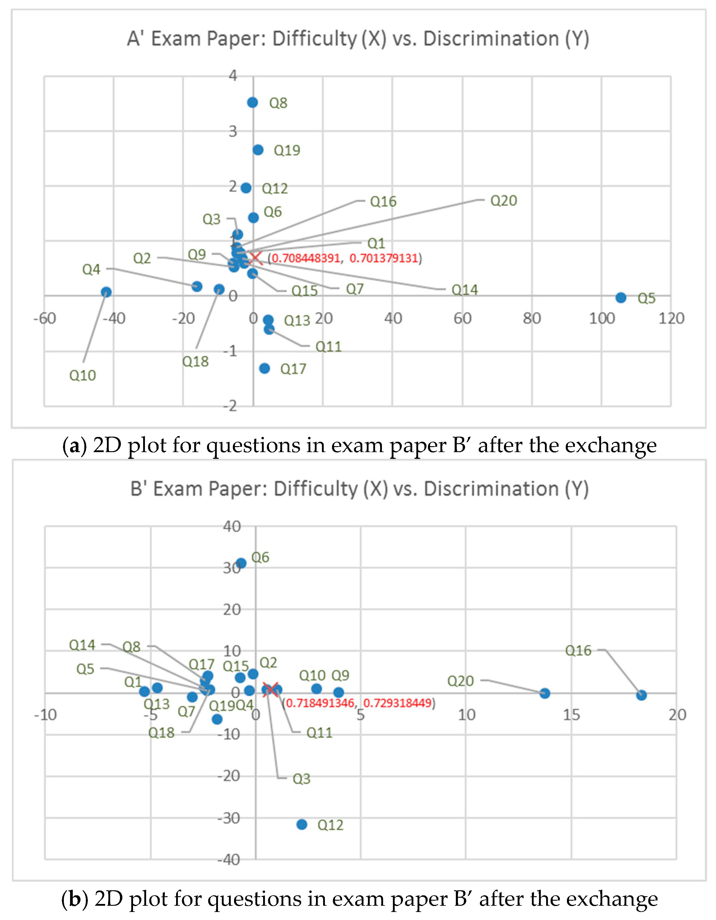
4.2. Distributions of Question Items in New Exam Papers

The discrimination and difficulty of the question items in each new exam paper are shown in Figure 4 without rescaling. The proposed model suggests that more moderately difficult questions should be moved to exam paper A’ (as most of the points in Figure 4a are distributed vertically around the Y axis) but more moderately discriminative questions should be moved to B’ (as most of the points in Figure 4b are distributed horizontally around the X axis).

A more interesting observation is that because the hardest question (i.e., Q5 whose difficulty index > 100) is included in A’, the model determines that three much easier questions should also be included (−50 < difficulty < −10; i.e., Q4, Q10 and Q18). This is not observed in B’, wherein two harder questions are included (10 < difficulty < 20; i.e., Q16 and Q20) but no question that is very easy is included (i.e., the easiest question in B’, Q1, has a difficulty value below −10).

It can be concluded that the model chooses to make a different setting strategy for each exam paper. However, this does not matter because these observations do not erode the fairness brought by the two new exam papers, as their overall difficulty and discriminative power indices are almost on par. As long as the pursued average difficulty and discrimination (see the red crosses in both figures) are fair, the distribution of the question items is not as important as the overall fairness provided by the new exam papers. Note that the analysis uses the per-question average difficulty and discrimination for illustration clarity. This is tantamount to using their total values because the score received for correctly answering each question is 5 points, out of 100.

4.3. The Role of Weights: A Further Analysis

The exchange plan mentioned above assumes no priority for the gaps to be minimised between two exam papers. In the model, ‘$w_1=w_2=w_3=1$’ can be viewed as a weight vector, $W=\left[\begin{array}{ccc}{w}_1& w_2& w_3\end{array}\right]=\left[\begin{array}{ccc}1/3& 1/3& 1/3\end{array}\right]$, which implies an equal weighting of the considerations of difficulty, discrimination and guessing under the weight postulation.

However, as the model is capable of taking into account the different preferences for these dimensions in teachers’ mind, the teacher group leader was interviewed to learn the opinion regarding the real preferential weights. With the stated preference of $W^{\prime }=\left[\begin{array}{ccc}{w}_1& w_2& w_3\end{array}\right]=\left[\begin{array}{ccc}0.5& 0.4& 0.1\end{array}\right]$, another (BGP–item exchange planning) model is reconstructed using this setting. As a result, as shown in

Table 6. The exchanging plan suggested by the weighted binary goal programing (BGP) model (compared to the unweighted one).

Qj in Exam Paper A	Planned Exchanges	Qj in Exam Paper B	Remark (yj)	Exchanges (Unweighted)	yj (Unweighted)
Q1	⇋	Q1	1	⇋	1
Q2	⇋	Q2	1	⇋	1
Q3		Q3	0	⇋	1
Q4	⇋	Q4	1		0
Q5	⇋	Q5	1		0
Q6	⇋	Q6	1		0
Q7	⇋	Q7	1		0
Q8	⇋	Q8	1	⇋	1
Q9		Q9	0		0
Q10		Q10	0	⇋	1
Q11	⇋	Q11	1	⇋	1
Q12	⇋	Q12	1		0
Q13		Q13	0	⇋	1
Q14		Q14	0	⇋	1
Q15		Q15	0	⇋	1
Q16	⇋	Q16	1		0
Q17	⇋	Q17	1	⇋	1
Q18		Q18	0	⇋	1
Q19		Q19	0		0
Q20	⇋	Q20	1		0
Summary			12		11

, another ‘exchange plan’ that produces another two new exam papers, A″ and B″, emerged.

It is obvious that the exchanging patterns the two plans suggest are quite diversified. In addition, a total of 11 question pairs should be exchanged with the dimensions being equally weighted (using W), while a total of 12 should be exchanged with those being weighted by human (using W’).

As is further compared in

Table 7. Effectiveness of the human-weighted setting in comparison with that of the equally-weighted settings.

Attributes of A″	Value	Gap	Attributes of B″	Value
$S\begin{array}{c}{A}^{\prime }\\ \mathrm{Discrimination}\end{array}$	14.52126	0.4285717	$S\begin{array}{c}{B}^{\prime }\\ \mathrm{Discrimination}\end{array}$	14.09269
$S\begin{array}{c}{A}^{\prime }\\ \mathrm{Difficulty}\end{array}$	14.27311	0.007420312	$S\begin{array}{c}{B}^{\prime }\\ \mathrm{Difficulty}\end{array}$	14.26569
$S\begin{array}{c}{A}^{\prime }\\ \mathrm{Guessing}\end{array}$	3.118394	0.3863955	$S\begin{array}{c}{B}^{\prime }\\ \mathrm{Guessing}\end{array}$	3.504789
Objective Val.		0.2558935
Attributes of A’	Value	Gap	Attributes of B’	Value
$S\begin{array}{c}{A}^{\prime }\\ \mathrm{Discrimination}\end{array}$	14.58637	0.5587864	$S\begin{array}{c}{B}^{\prime }\\ \mathrm{Discrimination}\end{array}$	14.02758
$S\begin{array}{c}{A}^{\prime }\\ \mathrm{Difficulty}\end{array}$	14.36983	0.2008591	$S\begin{array}{c}{B}^{\prime }\\ \mathrm{Difficulty}\end{array}$	14.16897
$S\begin{array}{c}{A}^{\prime }\\ \mathrm{Guessing}\end{array}$	3.304500	0.01418366	$S\begin{array}{c}{B}^{\prime }\\ \mathrm{Guessing}\end{array}$	3.318683
Objective Val.		0.257943

, the weighted total gap between A″ and B″ is 0.2558935 with the human-weighted setting. This differs slightly from the averaged gap between A’ and B’, which is 0.257943 (0.7738291 × 1/3), but the achievement is slightly better. Compared to the plan with the equally-weighted setting, the gap in difficulty between the two exam papers is greatly reduced (0.007420312 between A″ and B″ but 0.2008591 between A’ and B’). Their gap in discrimination has also been reduced (0.5587864 compared to 0.4285717).

Nevertheless, the gap in guessing has increased due to a leverage. With the human-weighted setting, the weight assigned to minimize the difficulty gap is the greatest (0.5), and that assigned to minimize the discrimination gap is also great (0.4). Thus, in comparison to the gaps between A’ and B’, the difficulty and discrimination gaps between A″ and B″ are reduced, i.e., the model emphasizes these two dimensions by following the order indicated by W’. Therefore, after a trade-off, the human-weighted model sacrificed the gap-minimization goal for the guessing dimension, as it has the lowest priority (0.1).

In the analysis above, considering human preferences obtains another exchange plan that could be more satisfactory. As the plan is altered by the way the test administrator prioritizes the dimensions, this confirms that the reconstructed model is effective, which further encourages the use of factual weights when the application of (BGP–item exchange planning) is required in any context. Another empirical insight gained from this analysis is that, similar to other studies about test compilation, test administrators usually place more emphasis on the question items’ difficulty and discriminative power, rather than the probability of guessing a right answer.

A Sensitivity Analysis

Given the encouraging results shown above, a question arose as to how the suggested exchange plan (and the model solution) would change, subject to a change in the weight vector. That is, what if the weights were neither assumed to be equal nor assigned by the head teacher through an investigation? A sensitivity analysis could serve the purpose of gaining further insights in this regard.

As less emphasis is usually placed on the parametric dimension of guessing, several sets of probable weights are supposed for the difficulty and discrimination dimensions. Every round in the experiment, the weight of difficulty is increased by 10% and the weight of discrimination is decreased by 10%, and vice versa (to determine the used weight portfolio). The experiment halts when any one of them receives an importance that is equal to the importance of guessing (or is less important than guessing). The direct results are shown in

Table 8. Effectiveness of the human-weighted setting in comparison with that of the equally-weighted settings: Gaps in each dimension and the total objective value under the different weight portfolios.

	Weight Portfolios Investigated
$\mathrm{Discr}.(w_1)$	10%	20%	30%	40%	50%	60%	70%	80%
$\mathrm{Diffi}.(w_2)$	80%	70%	60%	50%	40%	30%	20%	10%
$\mathrm{Guess}.(w_3)$	10%	10%	10%	10%	10%	10%	10%	10%
A’ Discr.	14.58637	14.58637	14.09269	14.31098	14.31098	14.30297	14.31098	14.31098
A’ Diffi.	14.36983	14.36983	14.26569	13.68014	13.68014	14.85866	13.68014	13.68014
A’ Guess.	3.30450	3.30450	3.50479	3.26494	3.26494	3.35825	3.26494	3.26494
B’ Discr.	14.02758	14.02758	14.52126	14.30297	14.30297	14.31098	14.30297	14.30297
B’ Diffi.	14.16897	14.16897	14.27311	14.85866	14.85866	13.68014	14.85866	14.85866
B’ Guess.	3.31868	3.31868	3.11839	3.35825	3.35825	3.26494	3.35825	3.35825
D. Discr.	0.55879	0.55879	0.42857	0.00801	0.00801	0.00801	0.00801	0.00801
D. Diffi.	0.20086	0.20086	0.00742	1.17852	1.17852	1.17852	1.17852	1.17852
D. Guess.	0.01418	0.01418	0.38640	0.09331	0.09331	0.09331	0.09331	0.09331
Obj. (Agg.)	0.05614	0.08073	0.10367	0.10914	0.08990	0.07066	0.05142	0.03218

. These results are further visualized and compared in Figure 5, with the number of questions exchanged and the detailed exchange plan given under each weight portfolio setting shown in

Table 9. Effectiveness of the human-weighted setting in comparison with that of the equally-weighted settings: The detailed exchange plan given under each weight portfolio setting and the total number of questions exchanged.

	$\mathbf{Weight}\mathbf{Portfolios}\mathbf{Investigated}({\mathit{w}}_3=10\%)$
$\mathrm{Discr}.(w_1)$	10%	20%	30%	40%	50%	60%	70%	80%
$\mathrm{Diffi}.(w_2)$	80%	70%	60%	50%	40%	30%	20%	10%
Exchanged Qs	Exchanging Details
Q1	X	X				X
Q2	X	X				X
Q3	X	X	X	X	X		X	X
Q4				X	X		X	X
Q5				X	X		X	X
Q6				X	X		X	X
Q7						X
Q8	X	X		X	X		X	X
Q9			X			X
Q10	X	X	X			X
Q11	X	X		X	X		X	X
Q12				X	X		X	X
Q13	X	X	X	X	X		X	X
Q14	X	X	X			X
Q15	X	X	X			X
Q16				X	X		X	X
Q17	X	X				X
Q18	X	X	X			X
Q19			X	X	X		X	X
Q20				X	X		X	X
#Qs Exchanged	11	11	8	11	11	9	11	11

.

The experiment mentioned above uses the extension model of the gap-minimization (BGP–IEP) model in Section 2.3, wherein the deviations connoting the goals in the objective are normalized according to Equation (2”). Referring to the study by Chang [54], in that paper, except for the bounds of the values of those item parameters, the ‘suitable ranges’ (see also Section 2.2) of these parameters were also induced, as: 0 ≤ a_j ≤ 2, −3 ≤ b_j ≤ 3 and 0 ≤ c_j ≤ 1. This implies a ratio of 2:6:1 of ‘suitable violation intervals’ for discrimination, difficulty and the guessing parameters. Therefore, specifically for the analytical purpose here, in Equation (2”), the normalization constants are set as ${\Delta }_1=2$, ${\Delta }_2=6$ and ${\Delta }_3=1$, respectively, according to the above ratio.

As can be observed in Table 9 and Figure 5b, the solution to the exchange plan converges at the two ends, i.e., when the weight of either discrimination or difficulty becomes less than that of guessing (i.e., {discrimination, difficulty} = {20%, 70%} and {10%, 80%}, or {70%, 20%} and {80%, 10%}). However, the solution ‘turns around’ at the setting when {discrimination, difficulty} = {30%, 60%}, and when {discrimination, difficulty} = {60%, 30%} (that is, it yields a different optimal solution and then yet another optimal solution across these barriers). Besides, either a weight portfolio of {discrimination, difficulty} = {40%, 50%} or {50%, 40%} also converges to the same solution, which is very like the solution when discrimination is heavily addressed (as compared to difficulty). For this item exchange planning case, this solution yields the best compromise when the consideration for discrimination and difficulty are almost on par. Due to a lack of space, other interesting insights from this analysis are awaiting further discussion and exploration.

4.4. Flow for Future Implementation of IRT–BGP

Based on these positive results, further application is expected. A more complete flow for the implementation of IRT–BGP is therefore suggested for holding a fair test using A/B exam papers without the use of question banks:

(1)

The teacher or teacher’s team construct both the original A and B exam papers, with each pair of questions being associated with a certain piece of knowledge.

(2)

A pre-test that uses the original papers is given to two individual random groups of students who are not the respondents in the real test.

(3)

The answers to all the questions in the pre-test are recorded, and the correctness of the answers is justified to form the data warehouse required for subsequent analysis.

(4)

Use IRT to estimate the guessing, difficulty and discrimination parameters for each item contained in A and B, based on the data available in (3).

(5)

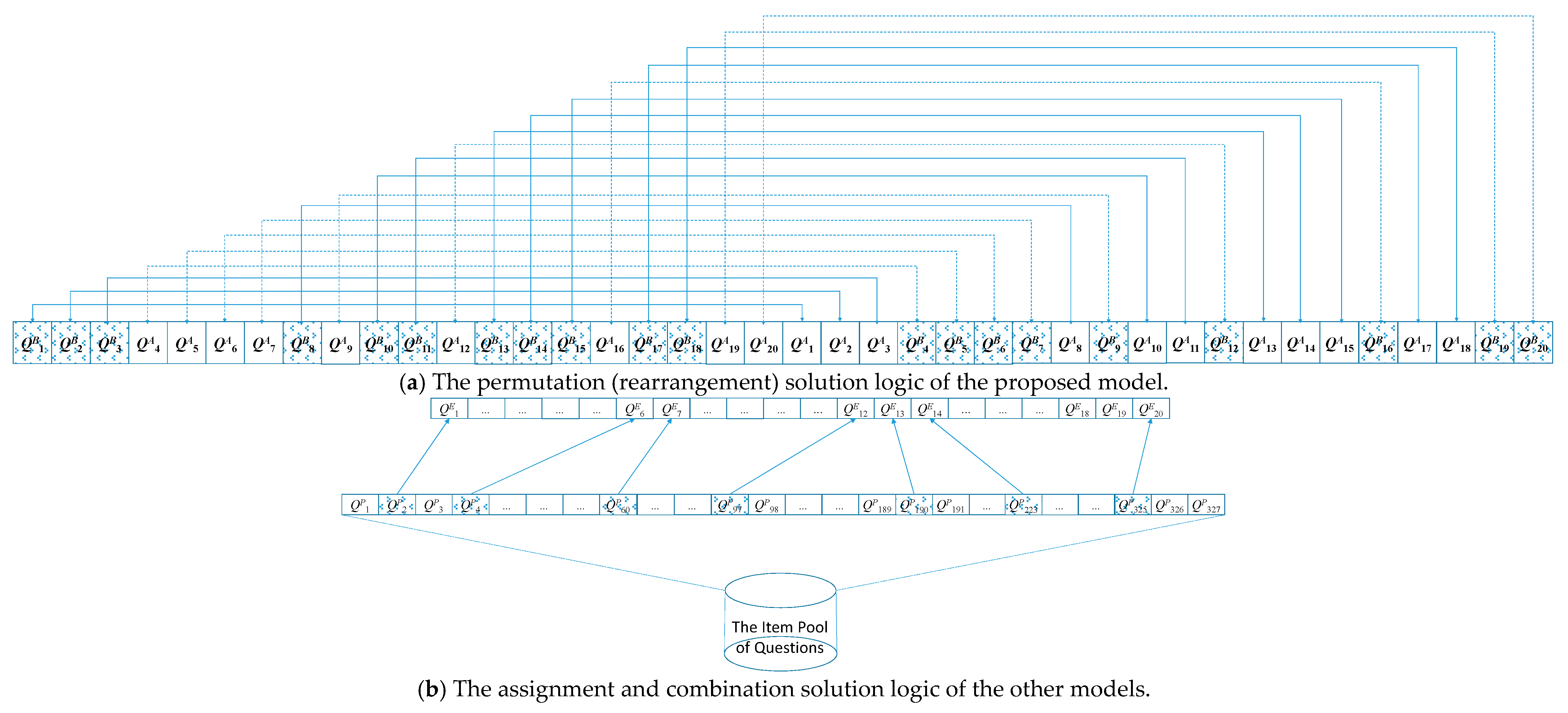
Build a (BGP–item exchange planning) model using the item parameters estimated in (4). Solve the model to determine an ‘exchange plan’. Obtain two new exam papers, A’ and B’ by reference to the plan.

(6)

The new A’ and B’ exam papers are used to test two student groups in the real A/B test.

Figure 6 depicts this flow and the way in which the flow is applied for teachers who are teaching a similar large general course but facing a similar problem. This acknowledges the request to set two exam papers ‘on the fly’ (to determine an exchange plan for the paired, associated questions that have just been set) to the fairest extent possible when there is no existing item pool from which questions can be retrieved, which is the main RQ of this study.

The pre-test requires a sample of students that is at least sufficient so that the results are statistically significant, e.g., the classical magic number based on the normal distribution, which is ≥ 32 [61]. In addition, one way to guarantee that test-takers with characteristics similar to those of the students enrolled in the real exam are included in the pre-test is to use a sample consisting of upper grade students who have also taken the same course. In this case, the safety requirements of having an exam previously tested using another sample of individuals can be met by asking the pre-test takers to sign a non-disclosure agreement.

Lastly, an extensive discussion is provided in terms of methodology. Following from Section 1.2.4, traditional test compilation is an organization problem of an (or several individual) exam paper(s), which is in fact an ‘assignment problem’. But the studied one is an ‘arrangement problem’ between exam papers, in the broader sense of ‘what is to be optimized’ for ‘combinatorial optimization’. This is true when the two original exam papers are stacked as one. Figure 7 clearly shows this difference as well as the logics thereof, clearly. The former is an assignment problem wherein the items drawn from a large pool are assigned to certain limited lots (as defined by the number of questions) in an exam paper, as long as the exam paper composed can meet the required standard. However, the latter is an arrangement problem wherein the existing questions are present but a balance between their placements is pursued. The figure shows that the new model’s goal is to re-permute the elements by exchanging each pair of (j, j + 20) elements and seeing whether this results in improvement. This permutation problem is an arrangement problem de facto.

5. Conclusions

This paper studies the niche problem of setting A/B exam papers fairly, subject to the absence of an existing item pool of questions. Accordingly, an IRT–BGP hybrid modelling approach is proposed (see the flowchart in Section 4.4). IRT is used to estimate the item parameters (i.e., guessing, difficulty and the discriminative power) of the questions included in both exam papers (A and B). These are then used as the model parameters of the proposed (BGP–item exchange planning) model, with the preferential weights manifested by the test administrators for the three item-parametric dimensions.

The solution provides an ‘exchange plan’ for the way the associated questions in two exam papers that are paired in terms of the point of knowledge to be tested should be exchanged. Two new exam papers (A’ and B’) are thus obtained, and they may achieve the desired leverages between the exam papers in the three dimensions, such that the two exam papers become as fair as possible for the students taking the exam. Therefore, the test becomes as fair as possible for the exam takers who are randomly allotted to participate in the test using either A’ or B’. The offered fairest (or almost fair) A/B test not only benefits the dynamically-grouped teacher’s team when A/B tests should be held but the teachers do not have the knowledge needed to intrinsically make these separate tests fair, subject to the usual context in educational practice in which there is no item pool available, but also implies many positive effects for both teachers and students from the perspectives of educational psychology (see the former discussions).

This study also offers a state-of-the-art empirical case for the studied problem. The source data was collected for a large general required course, which resulted in a solid sampling ground for subsequent analyses and the implications drawn. In addition, for this course the teaching team is dynamically organized year by year such that there is no common question item pool established (and is not necessary); however, the teachers are nonetheless asked to set A/B exam papers for the two term-test sessions. As such, the used case is sufficient to justify the proposed approach.

Some future research directions can be recommended. At first, despite the empirical finding that the unfairness of the test would be enormous if questions in the two original exam papers were not suitably balanced (which can be observed in Figure 1 and Table 1 and Table 2), and despite the finding that the proposed model may well balance the two exam papers by exchanging the paired associated questions (as shown in Table 4, Table 5 and Table 7), other observations can also be made if the flow suggested in Section 4.4 can be implemented. In this case, the teachers in the group will be asked to agree to alter the setting process for the exam papers used in a term test. The possible advantages can therefore be examined by statistically testing if distributions of the students’ scores (such as Figure 2) using the new A’ and B’ exam papers are improved (such that a true fair A/B test is given) and if the gap in the average scores is still significant.

The other possible direction is model enhancement. In this study, the model exchanges questions in two exam papers. However, in pedagogical practice, there are situations in which more than two exam papers, each of which is testing the same set of knowledge, should be used for a large-scale test but in which, meanwhile, the fairness of the test should remain unquestionable. Another situation would be one in which even though there are two exam papers, the two papers contain blocks of questions, such that the basic unit for item exchange would be question blocks, rather than individual items themselves. Under these circumstances, how to improve the model to leverage in the multiple item-parametric dimensions among more than two exam papers and exchange the given limited set of questions in these exam papers is the challenge.

Another further enhancement relates to the flexibility of the proposed model. In Section 2.3, the model’s generalized applications were discussed, as one can totally neglect some parameter(s) while pursuing that of fairness (between the exam papers). However, as in the field of GP, pre-emptive GP (PGP) is an approach that has been used to allot every goal into several prioritized goal sets, such that any neglected parametric dimension (e.g., guessing) can also be placed at a second priority level of PGP (i.e., and not just be neglected). In such cases, models such as PGP [62] or lexicographic GP [42] may be applied.

Yet another direction pertains to the future application of the BGP modelling approach to the traditional exam paper setting problems wherein a question bank exists and the aim is to retrieve a suitable set of questions that meets the required standard in each parametric dimension. Should this be the case, improvements in later works could be expected since GP is a special type of LP which can generate more information for multi-criteria decision analysis (MCDA).

Finally, it always requires supports for consistency and fairness in exam practice [63], so to assessments in other pedagogical activities. The approach presented in this study also serves this purpose.

References

1. Embretson, S.E.; Reise, S.P. Item Response Theory for Psychologists; Lawrence Erlbaum Associates: New Jersey, NJ, USA, 2013. [Google Scholar]
2. Firestone, W.A.; Donaldson, M.L. Teacher evaluation as data use: What recent research suggests. Educ. Assess. Eval. Account. 2019, 31, 289–314. [Google Scholar] [CrossRef]
3. Johnes, J. Operational research in education. Eur. J. Oper. Res. 2015, 243, 683–696. [Google Scholar] [CrossRef] [Green Version]
4. Saad, S.; Carter, G.W.; Rothenberg, M.; Israelson, E. Chapter 3: Understanding test quality—Concepts of reliability and validity. In Testing and Assessment: An Employer’s Guide to Good Practices by Employment and Training Administration; U.S. Department of Labour: Washington, DC, USA, 1999; pp. 1–11. [Google Scholar]
5. Wang, S.P.; Hsieh, Y.K.; Zhuang, Z.Y.; Ou, N.C. Solving an outpatient nurse scheduling problem by binary goal programming. J. Ind. Prod. Eng. 2014, 31, 41–50. [Google Scholar] [CrossRef]
6. Eignor, D.R. The standards for educational and psychological testing. In APA Handbooks in Psychology, APA Handbook of Testing and Assessment in Psychology; Geisinger, K.F., Bracken, B.A., Carlson, J.F., Hansen, J.-I.C., Kuncel, N.R., Reise, S.P., Rodriguez, M.C., Eds.; Test theory and testing and assessment in industrial and organizational psychology; American Psychological Association: Clark University, Worcester, MA, USA, 2013; Volume 1, p. 74. [Google Scholar] [CrossRef]
7. Helms, J.E. Fairness is not validity or cultural bias in racial-group assessment: A quantitative perspective. Am. Psychol. 2006, 61, 845. [Google Scholar] [CrossRef] [PubMed]
8. Camilli, G. Test fairness. Educ. Meas. 2006, 4, 221–256. [Google Scholar]
9. Shohamy, E. Performance assessment in language testing. Annu. Rev. Appl. Linguist. 1995, 15, 188–211. [Google Scholar] [CrossRef]
10. Shohamy, E. Critical language testing and beyond. Stud. Educ. Eval. 1998, 24, 331–345. [Google Scholar] [CrossRef]
11. Tan, P.J.-B. Students’ adoptions and attitudes towards electronic placement tests: A UTAUT analysis. Am. J. Comput. Technol. Appl. 2013, 1, 14–23. [Google Scholar]
12. Tan, P.J.-B.; Hsu, M. Designing a System for English Evaluation and Teaching Devices: A PZB and TAM Model Analysis. Eurasia J. Math. Sci. Technol. Educ. 2018, 14, 2107–2119. [Google Scholar] [CrossRef]
13. Berry, R.A.W. Novice teachers’ conceptions of fairness in inclusion classrooms. Teach. Teach. Educ. 2008, 24, 1149–1159. [Google Scholar] [CrossRef]
14. Ortner, T.M.; Weißkopf, E.; Gerstenberg, F.X. Skilled but unaware of it: CAT undermines a test taker’s metacognitive competence. Eur. J. Psychol. Educ. 2013, 28, 37–51. [Google Scholar] [CrossRef]
15. Paufler, N.A.; Clark, C. Reframing conversations about teacher quality: School and district administrators’ perceptions of the validity, reliability, and justifiability of a new teacher evaluation system. Educ. Assess. Eval. Account. 2019, 31, 33–60. [Google Scholar] [CrossRef]
16. Reimann, N.; Sadler, I. Personal understanding of assessment and the link to assessment practice: The perspectives of higher education staff. Assess. Eval. High. Educ. 2017, 42, 724–736. [Google Scholar] [CrossRef] [Green Version]
17. Skedsmo, G.; Huber, S.G. Measuring teaching quality: Some key issues. Educ. Assess. Eval. Account. 2019, 31, 151–153. [Google Scholar] [CrossRef] [Green Version]
18. Wei, W.; Yanmei, X. University teachers’ reflections on the reasons behind their changing feedback practice. Assess. Eval. High. Educ. 2018, 43, 867–879. [Google Scholar] [CrossRef]
19. Lord, F.M. The relation of test score to the trait underlying the test. Educ. Psychol. Meas. 1953, 13, 517–549. [Google Scholar] [CrossRef]
20. Sijtsma, K.; Junker, B.W. Item response theory: Past performance, present developments, and future expectations. Behaviormetrika 2006, 33, 75–102. [Google Scholar] [CrossRef]
21. Griffore, R.J. Speaking of fairness in testing. Am. Psychol. 2007, 62, 1081–1082. [Google Scholar] [CrossRef]
22. Miller, J.D. The measurement of civic scientific literacy. Public Underst. Sci. 1998, 7, 203–223. [Google Scholar] [CrossRef]
23. Bauer, M.W.; Allum, N.; Miller, S. What can we learn from 25 years of PUS survey research? Liberating and expanding the agenda. Public Underst. Sci. 2007, 16, 79–95. [Google Scholar] [CrossRef] [Green Version]
24. Bauer, M.W. Survey research and the public understanding of science. In Handbook of Public Communication of Science & Technology; Bucchi, M., Trench, B., Eds.; Routledge: New York, NY, USA, 2008; pp. 111–130. [Google Scholar]
25. Cajas, F. Public understanding of science: Using technology to enhance school science in everyday life. Int. J. Sci. Educ. 1999, 21, 765–773. [Google Scholar] [CrossRef]
26. Mejlgaard, N.; Stares, S. Participation and competence as joint components in a cross-national analysis of scientific citizenship. Public Underst. Sci. 2010, 19, 545–561. [Google Scholar] [CrossRef]
27. Kawamoto, S.; Nakayama, M.; Saijo, M. A survey of scientific literacy to provide a foundation for designing science communication in Japan. Public Underst. Sci. 2013, 22, 674–690. [Google Scholar] [CrossRef] [PubMed]
28. Miller, J.D.; Pardo, R. Civic scientific literacy and attitude to science and technology: A comparative analysis of the European Union, the United States, Japan, and Canada. In Between Understanding and Trust: The Public, Science, and Technology; Dierkes, M., von Grote, C., Eds.; Harwood Academic Publishers: Amsterdam, The Netherlands, 2000; pp. 81–129. [Google Scholar]
29. Wu, S.; Zhang, Y.; Zhuang, Z.-Y. A systematic initial study of civic scientific literacy in China: Cross-national comparable results from scientific cognition to sustainable literacy. Sustainability 2018, 10, 3129. [Google Scholar] [CrossRef] [Green Version]
30. Lord, F.M. Practical applications of item characteristic curve theory. J. Educ. Meas. 1977, 14, 117–138. [Google Scholar] [CrossRef]
31. Yen, W.M. Use of the three-parameter logistic model in the development of a standardized achievement test. In Applications of Item Response Theory; Hambleton, R.K., Ed.; Educational Research Institute of British Columbia: Vancouver, CO, Canada, 1983; pp. 123–141. [Google Scholar]
32. Theunissen, T.J.J.M. Binary programming and test design. Psychometrika 1985, 50, 411–420. [Google Scholar] [CrossRef]
33. Boekkooi-Timminga, E. Simultaneous test construction by zero-one programming. Methodika 1987, 1, 102–112. [Google Scholar]
34. Boekkooi-Timminga, E.; van der Linden, W.J. Algorithms for automated test construction. In Computers in Psychology: Methods, Instrumentation and Psychodiagnostics; Maarse, F.J., Mulder, L.J.M., Sjouw, W.P.B., Akkerman, A.E., Eds.; Swets & Zeitlinger: Lisse, The Netherlands, 1987; pp. 165–170. [Google Scholar]
35. Adema, J.J. Methods and models for the construction of weakly parallel tests. Appl. Psychol. Meas. 1992, 16, 53–63. [Google Scholar] [CrossRef] [Green Version]
36. Swanson, L.; Stocking, M.L. A model and heuristic for solving very large item selection problems. Appl. Psychol. Meas. 1993, 17, 151–166. [Google Scholar] [CrossRef] [Green Version]
37. Charnes, A.; Cooper, W.W. Multiple Criteria Optimization and Goal Programming. Oper. Res. 1975, 23, B384. [Google Scholar]
38. Aouni, B.; Ben Abdelaziz, F.; Martel, J.M. Decision-maker’s preferences modeling in the stochastic goal programming. Eur. J. Oper. Res. 2005, 162, 610–618. [Google Scholar] [CrossRef]
39. Chang, C.-T. Multi-choice goal programming. Omega Int. J. Manag. Sci. 2007, 35, 389–396. [Google Scholar] [CrossRef]
40. Chang, C.-T.; Chen, H.-M.; Zhuang, Z.-Y. Revised multi-segment goal programming: Percentage goal programming. Comput. Ind. Eng. 2012, 63, 1235–1242. [Google Scholar] [CrossRef]
41. Kettani, O.; Aouni, B.; Martel, J.M. The double role of the weight factor in the goal programming model. Comput. Oper. Res. 2004, 31, 1833–1845. [Google Scholar] [CrossRef]
42. Romero, C. Extended lexicographic goal programming: A unifying approach. Omega Int. J. Manag. Sci. 2001, 29, 63–71. [Google Scholar] [CrossRef]
43. Silva, A.F.D.; Marins, F.A.S.; Dias, E.X.; Miranda, R.D.C. Fuzzy Goal Programming applied to the process of capital budget in an economic environment under uncertainty. Gestão Produção 2018, 25, 148–159. [Google Scholar] [CrossRef] [Green Version]
44. Aouni, B.; Kettani, O. Goal programming model: A glorious history and a promising future. Eur. J. Oper. Res. 2001, 133, 225–231. [Google Scholar] [CrossRef]
45. Chang, C.-T.; Zhuang, Z.-Y. The Different Ways of Using Utility Function with Multi-Choice Goal Programming Transactions on Engineering Technologies; Springer: Dordrecht, The Netherlands, 2014; pp. 407–417. [Google Scholar]
46. Tamiz, M.; Jones, D.; Romero, C. Goal programming for decision making: An overview of the current state-of-the-art. Eur. J. Oper. Res. 1998, 111, 569–581. [Google Scholar] [CrossRef]
47. Caballero, R.; Ruiz, F.; Rodriguez-Uría, M.V.R.; Romero, C. Interactive meta-goal programming. Eur. J. Oper. Res. 2006, 175, 135–154. [Google Scholar] [CrossRef]
48. Chang, C.-T.; Chung, C.-K.; Sheu, J.-B.; Zhuang, Z.-Y.; Chen, H.-M. The optimal dual-pricing policy of mall parking service. Transp. Res. Part A Policy Pract. 2014, 70, 223–243. [Google Scholar] [CrossRef]
49. Colapinto, C.; Jayaraman, R.; Marsiglio, S. Multi-criteria decision analysis with goal programming in engineering, management and social sciences: A state-of-the art review. Ann. Oper. Res. 2017, 251, 7–40. [Google Scholar] [CrossRef] [Green Version]
50. Hocine, A.; Zhuang, Z.-Y.; Kouaissah, N.; Li, D.-C. Weighted-additive fuzzy multi-choice goal programming (WA-FMCGP) for supporting renewable energy site selection decisions. Eur. J. Oper. Res. 2020, 285, 642–654. [Google Scholar] [CrossRef]
51. Jones, D.; Tamiz, M. Goal programming in the period 1990–2000. In Multiple Criteria Optimization: State-of-the-Art Annotated Bibliographic Survey; Ehrgott, M., Gandibleux, X., Eds.; Kluwer Academic: Dordrecht, The Netherlands, 2002; pp. 130–172. [Google Scholar]
52. Sawik, B.; Faulin, J.; Pérez-Bernabeu, E. Multi-criteria optimization for fleet size with environmental aspects. Transp. Res. Procedia 2017, 27, 61–68. [Google Scholar] [CrossRef]
53. Zhuang, Z.-Y.; Su, C.-R.; Chang, S.-C. The effectiveness of IF-MADM (intuitionistic-fuzzy multi-attribute decision-making) for group decisions: Methods and an empirical assessment for the selection of a senior centre. Technol. Econ. Dev. Econ. 2019, 25, 322–364. [Google Scholar] [CrossRef]
54. Chang, W.-T. Research Digest: The Three-Parameter Logistic Model of Item Response Theory. E-papers of the National Academy of Educational Research (Taiwan, ROC). 2011. Volume 7. Available online: https://epaper.naer.edu.tw/index.php?edm_no=7 (accessed on 19 May 2020).
55. Romero, C. A general structure of achievement function for a goal programming model. Eur. J. Oper. Res. 2004, 153, 675–686. [Google Scholar] [CrossRef]
56. Romero, C. Handbook of Critical Issues in Goal Programming; Pergamon Press: São Paulo, Brazil, 2014. [Google Scholar]
57. Popper, K. The Logic of Scientific Discovery; Routledge: London, UK, 1992. [Google Scholar]
58. Martel, J.M.; Aouni, B. Incorporating the decision-maker’s preferences in the goal-programming model. J. Oper. Res. Soc. 1990, 41, 1121–1132. [Google Scholar] [CrossRef]
59. Lin, C.C. A weighted max—Min model for fuzzy goal programming. Fuzzy Sets Syst. 2004, 142, 407–420. [Google Scholar] [CrossRef]
60. Yaghoobi, M.A.; Tamiz, M. A method for solving fuzzy goal programming problems based on MINMAX approach. Eur. J. Oper. Res. 2007, 177, 1580–1590. [Google Scholar] [CrossRef]
61. Greenwood, J.A.; Sandomire, M.M. Sample size required for estimating the standard deviation as a per cent of its true value. J. Am. Stat. Assoc. 1950, 45, 257–260. [Google Scholar] [CrossRef]
62. Zeleny, M. The pros and cons of goal programming. Comput. Oper. Res. 1981, 8, 357–359. [Google Scholar] [CrossRef]
63. Klein, J. The failure of a decision support system: Inconsistency in test grading by teachers. Teach. Teach. Educ. 2002, 18, 1023–1033. [Google Scholar] [CrossRef]
64. Ignizio, J.P. Goal Programming and Extensions; Lexington Books: Lexington, MA, USA, 1976. [Google Scholar]
65. DeMars, C.E. Item information function. In SAGE Encyclopedia of Educational Research, Measurement, and Evaluation; Frey, B.B., Ed.; SAGE Publications Inc.: The Thousand Oaks, CA, USA, 2018; pp. 899–903. [Google Scholar] [CrossRef]
66. Moghadamzadeh, A.; Salehi, K.; Khodaie, E. A comparison the information functions of the item and test on one, two and three parametric model of the item response theory (IRT). Procedia Soc. Behav. Sci. 2011, 29, 1359–1367. [Google Scholar] [CrossRef] [Green Version]
67. Gulliksen, H. Theory of Mental Tests; Wiley: New York, NY, USA, 1950. [Google Scholar]
68. Birnbaum, A. Some latent trait models and their use in inferring an examinee’s ability. In Statistical Theories of Mental Test Scores (chapters 17–20); Lord, F.M., Novick, M.R., Eds.; Addison-Wesley: Boston, MA, USA, 1968. [Google Scholar]
69. Moustaki, I.; Knott, M. Generalized latent trait models. Psychometrika 2000, 65, 391–411. [Google Scholar] [CrossRef] [Green Version]
Figure 1. The flow of this study in terms of data-driven decision-making.
Mathematics 08 01290 g001
Figure 2. The distribution of students’ CAR-based scores. (a) Paper A, (b) Paper B.
Mathematics 08 01290 g002
Figure 3. Analyzing the exam papers in terms of difficulty and discrimination: the 2-dimensional plots.
Mathematics 08 01290 g003
Figure 4. 2D plot analysis of the discriminative power and difficulty of A’ and B’.
Mathematics 08 01290 g004
Figure 5. Results for implementation of different weight portfolios of discrimination and difficulty during optimization.
Mathematics 08 01290 g005
Figure 6. The flow incorporating the use of the proposed IRT-BGP hybrid model.
Mathematics 08 01290 g006
Figure 7. The solution logics: a comparison.
Mathematics 08 01290 g007