Equilibria and Stability of One Class of Positive Dynamic Systems with Entropy Operator: Application to Investment Dynamics Modeling

Abstract

Dynamical systems with entropy operator (DSEO) form a special class of dynamical systems whose nonlinear properties are described by the perturbed mathematical programming problem with entropy objective functions. A subclass of DSEO is the system with positive state coordinates (PDSEO), which are used as mathematical models of the spatiotemporal evolution of demographic and economic processes, dynamic image restoration procedures in computer tomography and machine learning. A mathematical model of the PDSEO with a connectivity parameter characterizing the influence of the entropy operator on the dynamic properties of the system is constructed. PDSEO can have positive stationary states of various classes depending on the number of positive components in the state vector. Classes with p positive components of the state vector ($p\le n$, where n is the order of the system) are considered. The framework of formal power series and the method of successive approximations for the formation of existence conditions of stationary states are developed. The conditions of existence are obtained in the form of relations between the parameters of the system. We used the method of differential Bellman inequalities to study the stability of classes of stationary states in a limited region of phase space. The parametric conditions of instability of the zero stationary state and p positive stationary states depending on the connectivity parameter are obtained. The framework of formal power series and the method of successive approximations for the formation of existence conditions and classification of stationary states are developed. The stability conditions “in large” stationary states are obtained, based on the method of differential Bellman inequalities. The developed methods of existence, classification and stability are illustrated by the analysis of the dynamic properties of the economic model with stochastic investment exchange. Positive stationary states characterize the profitability of economic subsystems. The conditions of profitability and their stability for all subsystems in the system and their various groups are obtained.

1. Introduction

Dynamic systems with an entropy operator are widely used for mathematical modeling of real processes. Apparently, research in this field was pioneered by A.J. Wilson [1], who suggested a thermodynamic approach to the mathematical modeling of transport and regional systems based on the hypothesis about the random nature of exchange processes and the existence of a stationary state that maximizes entropy. This approach turned out to be very fruitful, as is indicated by a large number of publications in which it was applied and further developed for modeling of macro systems [2], entropy restoration of tomographic images [3,4,5], demoeconomic modeling [6], machine learning [7] and others.

Of particular interest are dynamic processes with positive states. For their study, a fundamental principle of statistical thermodynamics—the principle of local equilibria—was developed. In accordance with this principle, a dynamic system is assumed to have “fast” and “slow” processes. A “fast” process is considered a sequence of locally stationary states that correspond to a “slow” process. There are many examples of such processes, but the main difficulties are connected with mathematical modeling of a “fast” process, i.e., with the description of a sequence of locally stationary states. The first idea introduced in [8] was to describe a “fast” process in terms of the local maximum of entropy that depends on the state of a corresponding “slow” process. This approach turned out to be very fruitful as well, and it was successfully applied in many problems, such as population dynamics modeling [9], the spatiotemporal development of settlements [10,11,12] and the dynamic entropy-based procedures of image restoration [13].

The integration of dynamic models of a “slow” process with entropy maximization models describing the locally stationary states of a “fast” process actually formed a new class of dynamic systems with the entropy operator (DSEO) [14]. Generally, the entropy operator in these systems was described by a perturbed mathematical programming problem with entropy objective functions that characterized the mapping of the state space of a “slow” process into the state space of a “fast” process. In most applications of positive dynamic systems with the entropy operator (PDSEO), the models of entropy operators of simpler form were used; namely, the ones described by perturbed problems of constrained entropy maximization. For this class of entropy operators, the conditions of existence, continuity, differentiation, and boundedness were obtained [15]. The Lipschitz constant is an important characteristic of an entropy operator that determines the dynamic properties of PDSEO. In [16,17], a linear majorant method was proposed and some estimates of the Lipschitz constant for the Fermi entropy operator were derived.

This paper is dedicated to the study of positive dynamic systems with the Boltzmann-type entropy operator and constraints on “fast” variables. The properties of a system are analyzed depending on the degree of influence of the entropy operator on them, which is characterized by the connectivity index. A method for calculating stationary positive states is developed and all such states are classified. Parametric conditions for the existence of positive stationary states and their stability in large are established. The proposed methods are used to study stationary states and their stability in an economic system that exchanges investments.

2. Positive Dynamic System with Entropy Operator

Positive dynamic systems are characterized by the state vector with nonnegative components. A subclass of such systems consists of positive dynamic systems with an entropy operator (PDSEO). The structural diagram of a PDSEO can be seen in Figure 1.

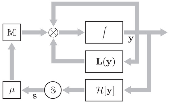
Figure 1. Functional diagram.

It includes three feedback loops with autonomous integrators as follows. One of them is the feedback loop by the state vector $\mathbf{y}\in R_{+}^n$ with the multiplying block $\mathbb{M}$; the other contains a nonlinear vector function $\mathbf{L}\left(\mathbf{y}\right)$ with components $L_1\left(y_1\right),\dots ,L_n\left(y_n\right)$; the third feedback loop incorporates an entropy operator $\mathcal{H}\left[\mathbf{y}\right]=X_{*}\left(\mathbf{y}\right)$, where $X_{*}$ is a nonnegative matrix of dimensions $(n\times n).$ The block $\mathbb{S}$ calculates the so-called $\mathbf{s}$-decrement of the matrix $X_{*}$, i.e., the difference between its column and row sums. The degree of influence of the entropy operator on the dynamic properties of the system is characterized by the connectivity index $\mu$.

The PDSEO under study is described by Equation [11]

$$\begin{array}{c}\dot{\mathbf{y}}=\mathbf{y}\otimes \left[\mathbf{L}\left(\mathbf{y}\right)+\mu \mathbf{s}\left(\mathbf{y}\right)\right],\mathbf{L}\left(\mathbf{y}\right)=\left\{L_i\left(y_i\right)\right|i=\overline{1,n}\}\hfill \\ \mathbf{s}\left(\mathbf{y}\right)=\left(X_{*}^{⊺}\left(\mathbf{y}\right)-X_{*}\left(\mathbf{y}\right)\right)\mathbf{e},\mathbf{e}=\{1,\dots ,1\}\in R^n\hfill \\ \mathcal{H}\left[\mathbf{y}\right]=X_{*}\left(\mathbf{y}\right)=argmax\left\{H\left(X\right)|0\le X\le C(\mathbf{y})\right\}\hfill \\ H\left(X\right)=-\mathrm{tr}\left(X{X}_{ln}\right),\hfill \end{array}$$

(1)

with the following notations: $\mathrm{tr}(•)$ as the trace of a matrix •; $X_{ln}$ as a matrix of dimensions $(n\times n)$ with elements $ln\frac{x_{ij}}{{\tilde{\nu }}_{ij}}$; ${\tilde{\nu }}_{ij}\in [0,1]$ and ${\sum }_{j=1}^n{\tilde{\nu }}_{ij}=1,i=\overline{1,n}$, as parameters; finally, $C\left(\mathbf{y}\right)$ as a matrix of dimensions $(n\times n)$ with elements $c_{ij}\left(\mathbf{y}\right)$.

Let us write system (1) in a more convenient form. Consider an entropy operator $\mathcal{H}\left(\mathbf{y}\right)$ described by a perturbed mathematical programming problem: maximize the Boltzmann information entropy [2] on the nonnegative polyhedron $0\le X\le C\left(\mathbf{y}\right)$. This problem can be simplified, i.e., reduced to an unconstrained maximization problem by passing to the entropy function

$$\tilde{H}\left(X\right)=-\mathrm{tr}\left\{\left(X{X}_{ln}\right)+\left[(C\left(\mathbf{y}\right)-X){(C\left(\mathbf{y}\right)-X)}_{ln}\right]\right\}.$$

(2)

The entropy function (2) structurally resembles the Fermi informational entropy [2]. As is easily observed, this function is defined on the above polyhedron, meaning that its absolute maximum belongs to the latter:

$$X_{*}\left(\mathbf{y}\right)=argmax\tilde{H}\left(X\right).$$

(3)

In accordance with (2), the elements of the matrix $X_{*}\left(\mathbf{y}\right)$ have the form

$$x_{ij}^{*}\left(\mathbf{y}\right)={\nu }_{ij}{c}_{ij}\left(\mathbf{y}\right),{\nu }_{ij}=\frac{{\tilde{\nu }}_{ij}}{1+{\tilde{\nu }}_{ij}}.$$

(4)

The vector of the $\mathbf{s}$-decrement of the matrix $X_{*}$ consists of the components

$$s_i\left(\mathbf{y}\right)=\sum _{j=1}^n\left({\nu }_{ji}{c}_{ji}\left(\mathbf{y}\right)-{\nu }_{ij}{c}_{ij}\left(\mathbf{y}\right)\right),i=\overline{1,n}.$$

(5)

Consider the case in which the functions $c_{ij}\left(\mathbf{y}\right)$ linearly depend on $y_i$:

$$c_{ij}\left(\mathbf{y}\right)={\alpha }_{ij}+{\beta }_{ij}{y}_i,(i,j)=\overline{1,n},$$

(6)

where ${\alpha }_{ij}$ and ${\beta }_{ij}$ are constant coefficients. In this case, the components of the vector $\mathbf{s}$ have the form

$$s_i\left(\mathbf{y}\right)=A_i-B_i{y}_i+\sum _{j=1}^n{\nu }_{ji}{\beta }_{ji}{y}_j,i=\overline{1,n},$$

(7)

where

$$A_i=\sum _{j=1}^n({\nu }_{ji}{\alpha }_{ji}-{\nu }_{ij}{\alpha }_{ij}),B_i=\sum _{j=1}^n{\nu }_{ij}{\beta }_{ij}.$$

(8)

Substituting these relations into Equation (1), we derive the PDSEO equation

$$\dot{\mathbf{y}}=\mathbf{y}\otimes \left(\mu \mathbf{A}+\tilde{\mathbf{L}}(\mathbf{y},\mu )+\mu B^{⊺}\mathbf{y}\right),$$

(9)

where the vector function $\tilde{\mathbf{L}}(\mathbf{y})$ consists of the components

$${\tilde{L}}_i(\mathbf{y},\mu )=-\mu B_i{y}_i+L_i\left(\mathbf{y}\right),i=\overline{1,n},$$

(10)

while the elements of the matrix B are ${\nu }_{ij}{\beta }_{ij}$.

Consider the PDSEO with

$$L_i\left(\mathbf{y}\right)=l_i^0+l_i{y}_i,i=\overline{1,n}.$$

(11)

Then Equation (9) takes the form

$$\dot{\mathbf{y}}=\mathbf{y}\otimes \left(D\left(\mu \right)\mathbf{y}+\mathbf{g}\left(\mu \right)\right),\mathbf{y}\left(0\right)\ge \mathbf{0},$$

(12)

where the elements of the matrix $D\left(\mu \right)$ are given by

$$d_{ij}\left(\mu \right)=\left\{\begin{array}{cc}{l}_i-\mu B_i\hfill & \mathrm{for}i=j,\hfill \\ \mu {\nu }_{ji}{\beta }_{ji}\hfill & \mathrm{for}i\ne j,\hfill \end{array}\right.$$

(13)

while the vector $\mathbf{g}\left(\mu \right)$ consists of the components

$$g_i\left(\mu \right)=l_i^0+\mu A_i.$$

(14)

Equations (12) with nonnegative initial conditions have a nonnegative solution, thereby representing an adequate model of the PDSEO.

3. Classification of Stationary States and Existence Conditions

An important problem connected with the study of PDSEOs is the existence of stationary states (equilibria) and their classification. The existence of stationary states depends on the degree of influence of the entropy operator on the dynamic properties of a system, i.e., on the connectivity index $\mu$. The stationary states of a PDSEO can be divided into three classes as follows.

The first class contains the unique trivial state $\mathbb{N}=\{{\mathbf{y}}^{*}=\mathbf{0}\}$. From Equation (12) it follows that this state always exists, regardless of the connectivity index.

The second class consists of the states with positive components of the state vector. Such a state will be called n-positive and denoted by ${\mathbb{P}}^n\left(\mu \right)=\{{\mathbf{y}}^{*}\left(\mu \right)>\mathbf{0}\}$.

Finally, the third class includes the states with $i_1,\dots ,i_p$ positive components of the state vector. Such states will be called $(i_1,\dots ,i_p)$-positive and denoted by ${\mathbb{P}}^{i_1,\dots ,i_p}\left(\mu \right)=\{y_{i_1}^{*}\left(\mu \right)>0,\dots ,y_{i_p}^{*}\left(\mu \right)>0;y_{k_1}^{*}\left(\mu \right)=0,\dots ,y_{k_{(n-p)}}^{*}\left(\mu \right)=0\}$, where the numbers $i_1,\dots ,i_p$ and $k_1,\dots ,k_{n-p}$ are different non-coinciding integers from the range $[1,n]$.

3.1. n-Positive States ${\mathbb{P}}^n\left(\mu \right)$

Consider system (11)–(13) with a fixed value of the connectivity index $\mu$. The matrix $D\left(\mu \right)$ is assumed to be nondegenerate, i.e., $detD\left(\mu \right)\ne 0$. Then the existence of a state ${\mathbb{P}}^n\left(\mu \right)$ of this system is determined by the existence of a positive solution to the linear equation

$$D\left(\mu \right)\mathbf{y}=-\mathbf{g}\left(\mu \right),\mathbf{y}\left(0\right)>\mathbf{0}.$$

(15)

In this case,

$${\mathbf{y}}^{*}\left(\mu \right)=-D^{-1}\left(\mu \right)\mathbf{g}\left(\mu \right)\ge \mathbf{0},\mu \in [0,1].$$

(16)

In particular, if $\mu =0$, then

$$y_i^{*}\left(0\right)=-\frac{l_i^0}{l_i}>0,i=1,\dots ,n.$$

(17)

Hence, for ${\mathbf{y}}^{*}\left(0\right)$ to be positive the parameters $l_i^0$ and $l^i$ must have different signs:

$$l_i^0\ge 0\&l_i\le 0,\mathrm{or}{l}_i^0\le 0\&l_i\ge 0,i=\overline{1,n}.$$

(18)

Consider the case in which $\mu (0,1]$. Reverting to Equation (15), we write it in the form

$$\left(D_1+\mu D_2+\mu D_3\right)\mathbf{y}=-{\mathbf{g}}^{\left(0\right)}-\mu {\mathbf{g}}^{\left(1\right)},$$

(19)

where:

—

the vectors ${\mathbf{g}}^{\left(0\right)}$ and ${\mathbf{g}}^{\left(1\right)}$ consist of the components $l_i^0$ and $A_i$, respectively;

—

the matrices $D_1$–$D_3$ are given by

$$D_1=\mathrm{diag}\left[l_i\right|i=\overline{1,n}],D_2=\mathrm{diag}\left[B_i\right|i=\overline{1,n}];$$

(20)

$$D_3\left(\mu \right)=\left(\begin{array}{cccc}0& B_{21}& \dots & B_{n1}\\ B_{12}& 0& \dots & B_{n2}\\ \dots & \dots & \dots & \dots \\ B_{1n}& B_{2n}& \dots & 0\end{array}\right).$$

(21)

Clearly, the matrix $D_3$ is degenerate, i.e., $det{D}_3=0$. We will construct the solution to Equation (19) as the formal series [18]

$${\mathbf{y}}^{*}\left(\mu \right)={\mathbf{y}}^{\left(0\right)}+\mu {\mathbf{y}}^{\left(1\right)}+{\mu }^2{\mathbf{y}}^{\left(2\right)}+\dots .$$

(22)

In this equality, the initial approximation ${\mathbf{y}}^{\left(0\right)}$ satisfies the equation

$$D_1{\mathbf{y}}^{\left(0\right)}=-{\mathbf{g}}^{\left(0\right)},{\mathbf{y}}^{\left(0\right)}={\mathbf{y}}^{*}\left(0\right);$$

(23)

the first approximation ${\mathbf{y}}^{\left(1\right)}\left(\mu \right),$ the equation

$$D_2{\mathbf{y}}^{\left(1\right)}=-{\mathbf{g}}^{\left(1\right)},{\mathbf{y}}^{\left(1\right)}=\left\{-\frac{A_1}{B_1},\dots ,-\frac{A_n}{B_n}\right\}.$$

(24)

Thus, in the first approximation the solution to (15) consists of the components

$$y_i^{*}\left(\mu \right)\cong -\frac{l_i^0}{l_i}-\mu \frac{A_i}{B_i},i=\overline{1,n}.$$

(25)

Direct analysis of the signs of all terms in these formulas allows us to establish the following result.

Theorem 1.

Suppose that

$$\begin{array}{c}\left\{(l_i^0\ge 0)\&(l_i\le 0)\left|\right|(l_i^0\le 0)\&(l_i\ge 0)\right\}\&\hfill \\ \left\{(A_i\ge 0)\&(B_i\le 0),\left|\right|(A_i\le 0)\&(B_i\ge 0)\right\}\hfill \\ i=\overline{1,n}.\hfill \end{array}$$

(26)

Then system (15) has the approximate ${\mathbb{P}}^n\left(\mu \right)$-state (25).

3.2. $(i_1,\dots ,i_p)$-Positive States ${\mathbb{P}}^{i_1,\dots ,i_p}\left(\mu \right)$

For identifying positive components in a state ${\mathbb{P}}^{i_1,\dots ,i_p}\left(\mu \right),$ we consider condition (26) with an appropriate modification. More specifically, we construct the matrix $D^{i_1,\dots ,i_p}\left(\mu \right)$ by removing the rows and columns with numbers $k_1,\dots ,k_{(n-p)}$ from the matrix $D\left(\mu \right).$ We perform the same procedure for the vector $\mathbf{g}\left(\mu \right)$ and denote the resulting truncated vector by ${\mathbf{g}}^{i_1,\dots ,i_p}\left(\mu \right)$. The existence conditions of a ${\mathbb{R}}^{i_1,\dots ,i_p}\left(\mu \right)$-state are also provided by Theorem 1, which should be formulated for the components of the state vector with numbers $i_1,\dots ,i_p.$

4. Stability of Stationary States

Now, we get back to the nonlinear Equation (12), for which there exists a stationary state ${\mathbf{y}}^{*}\left(\mu \right)$ from one of the above classes. For analyzing its stability, we introduce the deviation

$$\mathbf{x}\left(t\right)=\mathbf{y}\left(t\right)-{\mathbf{y}}^{*}\left(\mu \right)$$

(27)

and study the latter’s behavior as $t\to \infty .$

4.1. Stability of Trivial State

For this stationary state, the deviation is $\mathbf{x}\left(t\right)=\mathbf{y}\left(t\right)$, and the equation takes the form

$$\frac{d\mathbf{x}\left(t\right)}{dt}=\left[G\left(\mu \right)\mathbf{x}\left(t\right)+\mathbf{x}\left(t\right)\otimes D\left(\mu \right)\right]\mathbf{x}\left(t\right),$$

(28)

where

$$G\left(\mu \right)=\mathrm{diag}[g_i\left(\mu \right),i=\overline{1,n}].$$

(29)

We construct the transition matrix [19]

$$W_{\tau }^t\left(\mu \right)=exp\left(G\left(\mu \right)(t-\tau )\right).$$

(30)

Since the matrix $G\left(\mu \right)$ is diagonal with constant elements, the transition matrix is bounded by norm:

$$\parallel exp\left(G\left(\mu \right)(t-\tau )\right)\parallel \le exp\left(g_{max}\left(\mu \right)(t-\tau )\right),$$

(31)

where $\parallel •\parallel ={\left({\sum }_i{(•)}_i^2\right)}^{1/2}$ and

$$g_{max}\left(\mu \right)=\underset{i}{max}{g}_i\left(\mu \right)=\underset{i}{max}\left(l_i^0+\mu A_i\right).$$

(32)

Consider the integral equation that is equivalent to (28):

$$\mathbf{x}\left(t\right)=W_0^t\left(\mu \right)\mathbf{x}\left(0\right)+{\int }_0^t{W}_{\tau }^t\left(\mu \right)\left(\mathbf{x}\left(\tau \right)\otimes D\left(\mu \right)\mathbf{x}\left(\tau \right)\right)d\tau .$$

(33)

In view of (31), we may write [20]

$$\parallel \mathbf{x}\left(t\right)\parallel =u\left(t\right)\le v\left(t\right),$$

(34)

where

$$v\left(t\right)=exp\left(g_{max}\left(\mu \right)t\right)u\left(0\right)+{\int }_0^{t}exp\left(g_{max}\left(\mu \right)(t-\tau )\rho \left(\mu \right)u^2\left(\tau \right)\right)d\tau$$

(35)

and here we use designation $\parallel D\left(\mu \right)\parallel =\rho \left(\mu \right)$.

Differentiating this equality, we easily establish that the nonnegative variable $v\left(t\right)$ is the solution to the nonlinear differential equation

$$\dot{v}\left(t\right)=g_{max}\left(\mu \right)v\left(t\right)+\rho \left(\mu \right)v^2\left(t\right),v\left(0\right)=\parallel \mathbf{x}\left(0\right)\parallel >0.$$

(36)

The convergence ${lim}_{t\to \infty }v\left(t\right)=0$ holds if the right-hand side of this equation is negative:

$$v\left(t\right)\in [0,-g_{max}\left(\mu \right)/\rho \left(\mu \right)].$$

(37)

Because $v\left(t\right)$ is a nonnegative variable, $g_{max}\left(\mu \right)<0$. Since $g_{max}\left(\mu \right)$ is the maximum component of the vector $\mathbf{g}\left(\mu \right)$, all its components must satisfy the condition

$$g_i\left(\mu \right)=l_i^0+\mu A_i<0,i=1,\dots ,n.$$

(38)

Hence, the connectivity index is

$$\mu <-\frac{l_i^0}{A_i},i=\overline{1,n}.$$

(39)

Theorem 2.

Suppose that for all $i\in [1,n]$ the values $l_i^0$ and $A_i$ are simultaneously positive or simultaneously negative. Then there does not exist a value $\mu \in [0,1]$ that would satisfy at least one of the inequalities of system (39), and hence the trivial state $\mathbb{N}$ is unstable.

Corollary 1.

If for all $i\in [1,n]$ the values $l_i^0$ and $A_i$ have different signs, then for the connectivity indices $0<\mu <\frac{l_i^0}{A_i}$ the trivial state is stable.

4.2. Stability of Stationary States ${\mathbb{P}}^n\left(\mu \right)$

The differential equation in the deviation $\mathbf{x}\left(t\right)$ from a stationary state of the class ${\mathbb{P}}^n\left(\mu \right)$ has the form

$$\frac{d\mathbf{x}\left(t\right)}{dt}=R(\mu ,{\mathbf{y}}^{*})\mathbf{x}\left(t\right)+(\mathbf{x}\left(t\right)+{\mathbf{y}}^{*})\otimes \left[D\left(\mu \right)\mathbf{x}\left(t\right)\right],$$

(40)

where the elements of the matrix $D\left(\mu \right)$ are given by (13) and

$$R(\mu ,{\mathbf{y}}^{*})=\mathrm{diag}[g_i\left(\mu \right)+w_i(\mu ,{\mathbf{y}}^{*})],w_i\left({\mathbf{y}}^{*}\right)=\sum _{j=1}^n{d}_{ij}\left(\mu \right)y_j^{*}.$$

(41)

First of all, consider the case in which the connectivity index is $\mu =0$. In accordance with (13), (14), (17) and (18), we obtain

$$R(0,{\mathbf{y}}^{*})=0,D\left(0\right)=\mathrm{diag}\left[l_i\right|i=\overline{1,n}].$$

(42)

As a result, Equation (40) is transformed into

$$\frac{d{x}_i\left(t\right)}{dt}=l_i^0{x}_i\left(t\right)+l_i{x}_i^2\left(t\right),i=\overline{1,n}.$$

(43)

Theorem 3.

Suppose for all $i=\overline{1,n}$ the variables $l_i^0$ and $l_i$ have different signs. Then the state ${\mathbb{P}}^n\left(0\right)$ is asymptotically stable in the domain of initial deviations $\mathcal{X}={⨂}_{i=1}^n[0,-\frac{l_i^0}{l_i}]$.

The proof is straightforward: under the above hypotheses, the right-hand sides of Equation (43) take negative values in the domain $\mathcal{X}.$

Consider the case in which $\mu \ne 0$. We revert to Equation (40) for $0<\mu \le 1$ and adopt the approximate formula (22) for the stationary state ${\mathbb{P}}^n$.

Let the matrix $R(\mu ,{\mathbf{y}}^{*})$ in Equation (40) be Hurwitz stable, i.e.,

$${\lambda }_{max}=\underset{i\in [1,n]}{max}{g}_i\left(\mu \right)+w_i(\mu ,{\mathbf{y}}^{*})=g^{*}\left(\mu \right)+w^{*}(\mu ,{\mathbf{y}}^{*})<0,$$

(44)

and also let the matrix $D\left(\mu \right)$ have a finite norm $\rho \left(\mu \right)$.

We introduce the transition matrix

$$W_{\tau }^t(\mu ,{\mathbf{y}}^{*})=exp\left(R(\mu ,{\mathbf{y}}^{*})(t-\tau )\right).$$

(45)

Like before, the transition matrix is bounded by norm:

$$\parallel W_{\tau }^t(\mu ,{\mathbf{y}}^{*})\parallel \le exp(-{\lambda }_{max}(t-\tau )).$$

(46)

Using the transition matrix (45), we pass to the integral equation that is equivalent to the differential Equation (40):

$$\mathbf{x}\left(t\right)=W_0^t(\mu ,{\mathbf{y}}^{*})\mathbf{x}\left(0\right)+{\int }_0^t{W}_{\tau }^t(\mu ,{\mathbf{y}}^{*})\mathbf{x}\left(\tau \right)\otimes D\left(\mu \right)\mathbf{x}\left(\tau \right)d\tau .$$

(47)

The following bound is valid [20]:

$$\parallel \mathbf{x}\left(t\right)\parallel =u\left(t\right)\le v\left(t\right),v\left(t\right)=exp\left({\lambda }_{max}t\right)u\left(0\right)+{\int }_0^{t}exp\left({\lambda }_{max}(t-\tau )\right)\rho \left(\mu \right)u^2\left(\tau \right)d\tau .$$

(48)

Please note that the variables $u\left(t\right)$ and $v\left(t\right)$ are nonnegative. Differentiating the expression of $v\left(t\right)$ yields

$$\frac{dv\left(t\right)}{dt}={\lambda }_{max}exp\left({\lambda }_{max}t\right)u\left(0\right)+\rho \left(\mu \right)u^2\left(t\right)+{\left(\lambda \right)}_{max}{\int }_0^{t}exp\left({\lambda }_{max}(t-\tau )\right)\rho \left(\mu \right)u^2\left(\tau \right)d\tau .$$

(49)

A direct comparison of (48) and (49) indicates that $v\left(t\right)$ is the solution to the differential equation

$$\frac{dv\left(t\right)}{dt}={\lambda }_{max}v\left(t\right)+\rho \left(\mu \right)v^2\left(t\right).$$

(50)

Due to (48), we have the differential inequality

$$\frac{dv\left(t\right)}{dt}\le {\lambda }_{max}v\left(t\right)+\rho \left(\mu \right)v^2\left(t\right).$$

(51)

In accordance with the theorem on differential inequalities [20], $u\left(t\right)\le \tilde{v}\left(t\right)$, where $\tilde{v}\left(t\right)$ satisfies the differential equation

$$\frac{d\tilde{v}\left(t\right)}{dt}={\lambda }_{max}\tilde{v}\left(t\right)+\rho \left(\mu \right){\tilde{v}}^2\left(t\right),\tilde{v}\left(0\right)=u\left(0\right)=\parallel x\left(0\right)\parallel >0.$$

(52)

The right-hand side of this equation is negative if $\tilde{v}\left(0\right)\in [\rho \left(\mu \right)/{\lambda }_{max},0]$ (${\lambda }_{max}<0$). For any initial deviations from this range, $v\left(t\right)\to 0$ as $t\to \infty$.

Actually, we have established the following fact:

Theorem 4.

Suppose that the matrix $R(\mu ,{\mathbf{y}}^{*})$ in Equation (40) is Hurwitz stable and ${\lambda }_{max}<0$ is its maximum negative eigenvalue. Then the state ${\mathbb{P}}^n$ is asymptotically stable in the domain of initial deviations

$$\parallel \mathbf{x}\left(t\right)\parallel =u\in Dom(\mathbb{R},\mu )=[0,-\rho \left(\mu \right)/{\lambda }_{max}].$$

(53)

4.3. Stability of Stationary States ${\mathbb{P}}^{i_1,\dots ,i_p}\left(\mu \right)$

Theorem 4 also applies to the states from the class ${\mathbb{P}}^{i_1,\dots ,i_p}\left(\mu \right),$ with the only difference that the vector ${\mathbf{y}}^{*}=\{y_{i_1}^{*},\dots ,y_{i_p}^{*}\}$ and the matrices R and D are compiled from the rows of the original matrices with numbers $i_1,\dots ,i_p$.

5. Equilibria and Stability in Investment Dynamics Models

5.1. Model of Economic System with Investment Exchange

Consider an economic system composed of three subsystems $i=\overline{1,3}$ exchanging investments. The state of each subsystem is characterized by its investment-conditioned yield $Y_i\left(t\right)$ (output in value units) and total investments $I_i\left(t\right)$ (the sum of investments per unit time). The investment relations between the subsystems are an important economic indicator of their interaction, which is described by the connectivity index $\mu \in [0,1]$.

The investment balance of the economic system has the form

$$I_i\left(t\right)=N_i\left(t\right)+\mu [W_i\left(t\right)-E_i\left(t\right)],i=\overline{1,3},$$

(54)

with the following notations: $N_i\left(t\right)$ as the investment flow in own manufacture; $W_i\left(t\right)$ as the investment flow from other subsystems into subsystem i; finally, $E_i\left(t\right)$ as the investment flow from subsystem i into other subsystems. Denote by $x_{ij}\left(t\right)$ the investment flows from subsystem i into subsystem j. Then

$$E_i\left(t\right)=\sum _{j=1,j\ne i}^3{x}_{ij}\left(t\right),W_i\left(t\right)=\sum _{j=1,j\ne i}^3{x}_{ji}\left(t\right),i=\overline{1,3}.$$

(55)

Consider a random mechanism of investment flows between subsystems. Let the portions of investments be randomly and independently distributed among subsystems with some prior probabilities $a_{ij}.$ Please note that with a prior probability $a_{ii}\ne 0$ the portions of investments stay within subsystem i. In the aggregate, all portions of investments form the investment flow $N_i\left(t\right)$.

For each subsystem, the admissible investment flow is completely exhausted. Therefore, the probabilities $a_{ij}$ satisfy the constraint

$$\sum _{j=1}^3{a}_{ij}=1,i=\overline{1,3}.$$

(56)

We assume that the portions of investments are distributed rather fast, and hence at each time instant t the dynamics of this process can be considered a sequence of locally stationary states with the entropy [2,21]

$$H\left(X\left(t\right)\right)=-\sum _{i,j=1}^n{x}_{ij}\left(t\right)ln\frac{x_{ij}\left(t\right)}{a_{ij}}\Rightarrow max$$

(57)

subject to upper constraints on an admissible investment flow ${\tilde{I}}_i\left(t\right)$ for each subsystem. By definition, the admissible investment flow ${\tilde{I}}_i\left(t\right)>0$ depends on the yield of subsystem i. This dependence will be characterized by functions ${\phi }_i\left(Y_i\left(t\right)\right)>0$. As is well-known, initial investments are required for the operation of an economic system, which are not connected with yield. At initial stages of system operation, there may be no yield at all. Therefore, the functions ${\phi }_i\left(Y_i\left(t\right)\right)$ have a constant term ${\alpha }_i>0$ and also a variable term ${\tilde{\phi }}_i\left(Y_i\right)>0$ that linearly depends on yield (in first approximation), i.e.,

$${\phi }_i\left(Y_i\left(t\right)\right)={\alpha }_i+{\beta }_i{Y}_i\left(t\right),{\alpha }_i>0,{\beta }_i>0;i=\overline{1,3}.$$

(58)

Using the functions ${\phi }_i\left(Y_i\left(t\right)\right)$, we write the corresponding system of constraints on the investment activity of all subsystems as

$$\sum _{j=1}^n{x}_{ij}\left(t\right)={\phi }_i\left(Y_i\left(t\right)\right),i=\overline{1,3}.$$

(59)

The entropy operator that maps the space of yields into the space of investment flow matrices is described by the perturbed constrained maximization problem of entropy (57) on set (59). In view of relations (56), the solution to this problem has the form

$$x_{ij}^{*}\left(t\right)=a_{ij}{\phi }_i\left(Y_i\left(t\right)\right),(i,j)=\overline{1,3}.$$

(60)

Please note that the own investment flows $N_i\left(t\right)$ in (54) are given by

$$N_i\left(t\right)=a_{ii}{\phi }_i\left(Y_i\left(t\right)\right),i=\overline{1,3}.$$

(61)

The total investment flow makes up

$$I_i\left(t\right)=A_{ii}{\phi }_i\left(Y_i\right)+\mu \sum _{j\ne i}^n{a}_{ji}{\phi }_j\left(Y_j\left(t\right)\right),i=\overline{1,3},$$

(62)

where

$$A_{ii}=a_{ii}(1+\mu )-\mu .$$

(63)

Now, consider the phenomenology of yield dynamics, taking into account that this variable is nonnegative. A change in yield occurs under the influence of two oppositely directed processes: the depreciation of yield due to its consumption (accumulation) and the update of yield through investments. To ensure the nonnegativity of yield, for convenience its variability can be interpreted in terms of the relative rate of change $V_y\left(t\right)={\dot{Y}}_i\left(t\right)/Y_i\left(t\right).$ In the first approximation, the relative rate of change $V_y\left(y\right)$ is proportional to the difference in the aging rates, due to depreciation and update, through investments. Assuming that each of the listed components of the rate of change $V_y\left(t\right)$ is in turn proportional to the yield $Y_i\left(t\right)$ with a coefficient $s_i$ and also to the total investment flow $I_i\left(t\right)$ with a coefficient $b_i$, we can write the balance relation

$$V_y\left(t\right)=-s_i{Y}_i\left(t\right)+b_i{I}_i\left(t\right),Y_i\left(0\right)>0,i=\overline{1,3}.$$

(64)

Substituting the total investments expression (62) into this relation, we obtain the following system of nonlinear differential equations describing yield dynamics in the economic system composed of three interacting subsystems:

$$\frac{d{Y}_i\left(t\right)}{dt}=Y_i\left(t\right)[-s_i{Y}_i\left(t\right)+A_{ii}{\phi }_i\left(Y_i\right)+\mu \sum _{j\ne i}^n{a}_{ji}{\phi }_j\left(Y_j\left(t\right)\right)],Y_i\left(0\right)>0.i=\overline{1,3}.$$

(65)

Suppose that the total investments are linearly connected with yield (58). In this case, the above system of nonlinear differential equations takes the form

$$\frac{d{Y}_i\left(t\right)}{dt}=Y_i\left(t\right)[\sum _{j=1}^3{d}_{ij}\left(\mu \right)Y_i\left(t\right)+c_i\left(\mu \right)],Y_i\left(0\right)>0,i=\overline{1,3}.$$

(66)

Here the vector c consists of the components

$$c_i\left(\mu \right)=a_{ii}{\alpha }_i+\mu (\sum _{j=1}^n{a}_{ji}{\alpha }_j-{\alpha }_i),$$

(67)

and the elements of the matrix $D\left(\mu \right)$ are given by

$$d_{ij}\left(\mu \right)=\left\{\begin{array}{cc}\mu a_{ji}{\beta }_j\hfill & \mathrm{for}j\ne i,\hfill \\ -s_i+a_{ii}{\beta }_i(1+\mu )-\mu {\beta }_i\hfill & \mathrm{for}j=i.\hfill \end{array}\right.$$

(68)

System (66) with positive initial conditions (nonzero initial yield) has nonnegative solutions.

5.2. Model Parameters

These parameters are an illustration of the PDSEO analysis. The yields produced in each subsystem are depreciated with specific rates $s_1=0.07[1/year],s_2=0.03[1/year]$ and $s_3=0.1[1/year]$. All yields are measured in $\${10}^{10}.$

The random exchange of investments is described by the prior probability matrix

$$A=\left(\begin{array}{ccc}0.3& 0.6& 0.1\\ 0.1& 0.6& 0.3\\ 0.2& 0.1& 0.7\end{array}\right)$$

(69)

The parameters of the functions ${\phi }_i\left(Y_i\right)$ are presented in Table 1.

Table 1. Parameters of functions ${\phi }_i\left(Y_i\right)$.

i	1	2	3
$\alpha$	1.50	0.75	0.50
$\beta$	0.06	0.03	0.04

5.3. Analysis of Stationary States: Existence and Stability

Of economic interest are the states ${\mathbb{P}}^3\left(\mu \right)$ in which the yields in all subsystems are positive. In economic literature, such states are called full profitability states. The dependence of full profitability states and their stability on the connectivity index $\mu$ is illustrated in Table 2. Clearly, such states exist and are stable only for the values $\mu \in [0,0.681].$ For $\mu >0.681,$ they do not exist. The following notations are adopted in this table: $\mathrm{Dom}$ as the stability domain (53); $\mathrm{Stb}$ as the stability indicator, + for stable and − for unstable; ${\lambda }_{max}$ as the maximum eigenvalue.

Table 2. Full profitability states.

$\mathit{\mu }$	0	0.1	0.2	0.4	0.6	0.681	0.682	0.8	1.0
$Y_1^{*}$	8.65	6.75	5.15	2.61	0.67	0.005	−0.003	−0.87	2.12
$Y_2^{*}$	37.5	41.03	43.21	45.26	45.66	45.58	45.57	45.29	44.56
$Y_3^{*}$	4.86	5.65	6.44	7.93	9.27	9.76	9.77	10.44	11.47
$Dom$	4.22	4.19	3.18	1.66	0.43	0.004	−	−	−
$Stb$	+	+	+	+	+	+	−	−	−
${\lambda }_{max}$	−0.379	−0.391	−0.309	−0.175	−0.05	−0.0004	0.0002	0.07	0.189

The dependence of the stationary yields of different subsystems on the connectivity index ($Y_1^{*}\left(\mu \right),Y_2^{*}\left(\mu \right),Y_3^{*}\left(\mu \right)$) and also the stability domains ($Do{m}^{*}\left(\mu \right)$) are shown in Figure 2. Please note that these states exist for $\mu =[0,1]$ and are stable up to ${\mu }^{*}=0.681$.

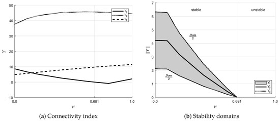
Figure 2. Full profitability states.

Now, consider $(i_1,i_2)$-profitability states (${\mathbb{R}}^{(i_1,i_2)}$). There may exist three states from this class, namely

$(2,3)$: $Y_1^{*}=0,Y_2^{*}>0,Y_3^{*}>0$;

$(1,3)$: $Y_1^{*}>0,Y_2^{*}=0,Y_3^{*}>0$;

$(1,2)$: $Y_1^{*}>0,Y_2^{*}>0,Y_3^{*}=0$;

The dependence of $(2,3),(1,3),(1,2)$-profitability states on the connectivity index is illustrated in Table 3, Table 4 and Table 5.

Table 3. The $\left(23\right)$-profitability states.

$\mathit{\mu }$	0	0.2	0.4	0.51	0.52	0.6	0.8	1.0
$Y_1^{*}$	0	0	0	0	0	0	0	0
$Y_2^{*}$	37.5	40.63	43.0	44.09	44.2	44.9	45.58	47.83
$Y_3^{*}$	4.86	6.29	7.74	8.54	8.75	9.18	9.77	11.97
$Dom$	−	−	−	−	0.045	0.654	1.24	3.17
$Stb$	−	−	−	−	+	+	+	+
${\lambda }_{max}$	0.45	0.275	0.1	0.004	−0.005	−0.075	−0.147	−0.425

Table 4. The $\left(13\right)$-profitability states.

$\mathit{\mu }$	0	0.2	0.4	0.54	0.545	0.6	0.8	1.0
$Y_1^{*}$	8.65	4.69	1.72	0.046	−0.008	−0.59	−2.44	−3.96
$Y_2^{*}$	0	0	0	0	0	0	0	0
$Y_3^{*}$	4.86	5.38	5.78	6.01	6.02	6.1	6.35	6.56
$Dom$	−	−	−	−	−	−	−	−
$Stb$	−	−	−	−	−	−	−	−
${\lambda }_{max}$	0.45	0.58	0.71	0.8	0.81	0.84	0.97	1.1

Table 5. The $\left(12\right)$-profitability states.

$\mathit{\mu }$	0	0.2	0.4	0.6	0.605	0.61	0.8	1.0
$Y_1^{*}$	8.65	4.98	2.22	0.05	0.001	−0.047	−1.72	−3.21
$Y_2^{*}$	37.5	42.77	44.17	43.8	43.78	43.76	42.61	41.01
$Y_3^{*}$	0	0	0	0	0	0	0	0
$Dom$	−	−	−	−	−	−	−	−
$Stb$	−	−	−	−	−	−	−	−
${\lambda }_{max}$	0.35	0.395	0.44	0.485	0.486	0.487	0.53	0.575

From these tables it follows that the $\left(23\right)$-profitability states exist for all values of the connectivity indices, but they are stable only for $\mu \ge 0.515$; the $\left(13\right)$-profitability states exist for $\mu \le 0.54$, but are unstable; the $\left(12\right)$-profitability states exist for $\mu \le 0.605.$

The last class of states consists of $1,2,3$-profitability states.

The dependence of $\left(1\right)$-profitability states on the connectivity index is illustrated in Table 6.

Table 6. The $\left(1\right)$-profitability states.

$\mathit{\mu }$	0	0.2	0.4	0.514	0.52	0.6	0.8	1.0
$Y_1^{*}$	8.65	4.55	1.45	0.003	−0.068	−0.97	−2.92	−4.52
$Y_2^{*}$	0	0	0	0	0	0	0	0
$Y_3^{*}$	0	0	0	0	0	0	0	0
$Dom$	−	−	−	−	−	−	−	−
$Stb$	−	−	−	−	−	−	−	−
${\lambda }_{max}$	0.45	0.58	0.71	0.784	0.788	0.84	0.97	1.1

From Table 6 it can be observed that the 1-profitability states exist for the connectivity index $\mu \in [0,0.514],$ but sufficient stability conditions for them are not satisfied.

The dependence of $\left(2\right)$-profitability states on the connectivity index is illustrated in Table 7.

Table 7. The $\left(2\right)$-profitability states.

$\mathit{\mu }$	0	0.2	0.4	0.6	0.8	1.0
$Y_1^{*}$	0	0	0	0	0	0
$Y_2^{*}$	37.5	40.28	42.26	43.75	44.91	45.83
$Y_3^{*}$	0	0	0	0	0	0
$Dom$	−	−	−	−	−	−
$Stb$	−	−	−	−	−	−
${\lambda }_{max}$	0.45	0.395	0.44	0.485	0.53	0.57

From Table 7 it can be observed that the 2-profitability states exist for all values of the connectivity index $\mu \in [0,1],$ but sufficient stability conditions for them are not satisfied.

The dependence of $\left(3\right)$-profitability states on the connectivity index is illustrated in Table 8.

Table 8. The $\left(3\right)$-profitability states.

$\mathit{\mu }$	0	0.2	0.4	0.6	0.8	1.0
$Y_1^{*}$	0	0	0	0	0	0
$Y_2^{*}$	0	0	0	0	0	0
$Y_3^{*}$	4.86	5.31	5.73	6.12	6.49	6.84
$Dom$	−	−	−	−	−	−
$Stb$	−	−	−	−	−	−
${\lambda }_{max}$	0.45	0.58	0.71	0.84	0.97	1.1

From Table 8 it can be observed that the 3-profitability states exist for all values of the connectivity index $\mu \in [0,1],$ but sufficient stability conditions for them are not satisfied.

Thus, the complete range of the connectivity index can be divided into the following subintervals:

• $[0,0.515),$ on which all types of stationary states exist, but only full profitability states are stable;
• $[0.515,0.542),$ on which all types of stationary states exist, except for the $\left(1\right)$-profitability ones; full and $\left(23\right)$-profitability states are stable;
• $[0.542,0.607),$ on which all types of stationary states exist, except for the $\left(1\right)$- and $\left(13\right)$-profitability ones; full and $\left(23\right)$-profitability states are stable;
• $[0.607,0.681),$ on which full-, $\left(23\right)$-, $\left(2\right)$- and $\left(3\right)$-profitability states exist; full and $\left(23\right)$-profitability states are stable.

6. Discussion and Future Work

The proposed method for the analysis of stationary states is based on an approximate solution of the stationary equations, which is constructed using a formal power series with respect to the connectivity parameter $\mu$. The first order approximation is used. It would be useful to study higher-order approximations, which would clarify the obtained conditions for the existence of positive stationary states.

The PDESO mathematical model contains the simplest Boltzmann entropy operator whose mathematical model taking into account the interval constraints on the variables transforms into the Fermi information entropy maximization problem.

However, in many applied problems in the above areas, mathematical models of PDSEO arise with equalities and inequalities conditions, which have more diverse dynamic properties, namely periodic, non-periodic modes and chaotic attractors.

7. Conclusions

A mathematical model of a positive dynamical system with an entropy operator was formed, focused on studying the influence of the entropy operator on the dynamic properties of the system. A classification of positive stationary states is given and the conditions for their existence are obtained. A theorem on the instability of the zero stationary state is proved. Using the method of differential Bellman inequalities, stability conditions “in large” of positive stationary states are obtained. For the model of the economic system of stochastic investment exchange, the concept of positive profitability conditions is introduced and the conditions for their existence and stability are obtained.

The results obtained can serve as the basis for the study of PDSEO with other classes of entropy operators, for example, the Fermi-entropy operator.

References

- Wilson, A.G. Entropy in Urban and Regional Modelling; Pion Ltd.: London, UK, 1970. [Google Scholar]
- Popkov, Y.S. Teoriya Makrosistem. Ravnovesnye Modeli; (Theory of Macrosystems. Equilibrium Models); URSS: Moscow, Russia, 1999. [Google Scholar]
- Herman, G.T. Image Reconstruction from Projections: The Fundamentals of Computerized Tomography; Academic Press: New York, NY, USA, 1980. [Google Scholar]
- Censor, Y.; Segmon, J. On Block-Iterative Entropy Optimization. J. Inf. Optim. Sci. 1987, 8, 275–291. [Google Scholar]
- Burne, C.L. Block-iterative Method for Image Reconstruction from Projections. IEEE Trans. Img. Proc. 1996, 5, 792–794. [Google Scholar] [CrossRef] [PubMed]
- Popkov, Y.S. Mathematical Demoeconomy: Integrating Demographic and Economic Approaches; De Gruiter GmbH: Berlin, Germany, 2014. [Google Scholar]
- Popkov, Y.S.; Popkov, A.Y.; Dubnov, Y.A. Randomizirovannoe Mashinnoe Obuchenie; (Randomized Machine Learning); LENAND: Moscow, Russia, 2019. [Google Scholar]
- Popkov, Y.S.; Ryazantsev, A.N. Spatio-Functional Models of Demographic Processes; UN Fund for Population Activity: New York, NY, USA, 1980; Preprint. [Google Scholar]
- Popkov, Y.S.; Shvetsov, V.I. A Principle of Local Equilibrium in the Regional Dynamic Models. Math. Model. 1990, 2, 40–50. [Google Scholar]
- Wilson, A.G. Catastrophe Theory and Bifurcations. Application to Urban and Regional Systems; Croom Helm: London, UK, 1981. [Google Scholar]
- Popkov, Y.S.; Shvetsov, V.I.; Weidlich, W. Settlement Formation Models with Entropy Operator. Ann. Reg. Sci. 1998, 32, 267–294. [Google Scholar] [CrossRef]
- Fan, Y.; Guo, R.; He, Z.; Li, M.; He, B.; Yang, H.; Wen, N. Spatio-temporal Pattern of Urban System Network in the Huaihe River Basin Based on Entropy Theory. Entropy 2019, 21, 20. [Google Scholar] [CrossRef]
- Popkov, Y.S.; Rublev, M.V. Dynamic Procedures of Image Reconstruction from Projections (Computer Tomography). Autom. Remote Control 2006, 67, 233–241. [Google Scholar] [CrossRef]
- Popkov, Y.S. Theory of Dynamic Entropy-operator Systems and Its Applications. Autom. Remote Control 2006, 67, 900–926. [Google Scholar] [CrossRef]
- Popkov, A.Y.; Popkov, Y.S.; Van Wissen, L. Positive Dynamic Systems with Entropy Operator: Application to Labour Market Modelling. EJOR 2005, 164, 811–828. [Google Scholar] [CrossRef]
- Popkov, Y.S. Upper Bound Design for Lipschitz Constant of the F(ν,q)-Entropy Operator. Mathematics 2018, 6, 73. [Google Scholar] [CrossRef]
- Popkov, Y.S. Method of Linear Majorant in the Theory of Monotonic Entropy Operators. Dokl. Math. 2018, 97, 277–278. [Google Scholar] [CrossRef]
- Krasnosel’skii, M.A.; Vainikko, G.M.; Zabreyko, R.P.; Ruticki, Y.B.; Stet’senko, V.Y. Approximate Solution of Operator Equations; Springer: Dordrecht, The Netherlands, 1972; p. 496. [Google Scholar]
- Tikhonov, A.N.; Vasil’eva, A.B.; Sveshnikov, A.G. Differentsial’nye Uravneniya; (Differential Equations); Fizmatlit: Moscow, Russia, 2005. [Google Scholar]
- Beckenbach, E.F.; Bellman, R. Inequalities; Springer: Berlin/Heidelberg, Germany, 1961. [Google Scholar]
- Puu, T. Nonlinear Economic Dynamics; Springer: Berlin/Heidelberg, Germany, 1997. [Google Scholar]
© 2020 by the author. Licensee MDPI, Basel, Switzerland. This article is an open access article distributed under the terms and conditions of the Creative Commons Attribution (CC BY) license (http://creativecommons.org/licenses/by/4.0/).