An Evaluation Model for Property-Purchasing Plans Based on a Hybrid Multi-Criteria Decision-Making Model

Abstract

Purchasing a property entails making rankings, comparisons, and trade-offs among various housing characteristics. When trying to sell a house, real estate brokers take on an important role as a middle-person between the seller and buyer. Thus, this research sets up a dynamic price recommendation method for housing purchases and applies the fuzzy multiple criteria decision making (FMCDM) technique, so as to realize housing quality and evaluation. We utilize this method based on the prospect theory of the loss aversion effect, in order to aid real estate brokers’ job of coordinating between the seller and buyer. The method helps us to provide an objective view of the evaluation matrix. From the pricing strategy, the results are able to match price versus quality and improve brokers’ intermediation effects. The brokers can subsequently make recommendations regarding a suitable price, decisions on negotiation strategies to reach an agreement, and settle upon an acceptable price.

1. Introduction

Purchasing a home is an important decision and perhaps one of the biggest expenses in most people’s lifetime. A great amount of time and lots of efforts are expected for buyers to find suitable homes in any real estate market, particularly in an urban area. The decision to purchase a home depends on a number of factors that vary for different housing markets and geographical areas. The buyer mainly considers the estimated value of performance/cost. Monroe and Chapman [1] denote consumers’ perceived value as being a psychological trade-off between the gains and sacrifices that they expect in transactions, as the desirability of a home depends on their needs and purchasing ability (i.e., income). The economic situation of a household also significantly affects its consumption through aspiration level and social comparison [2,3].

In the real estate market, various methods interpret quantitative and qualitative criteria to evaluate and make comparisons. The most common one is the Comparative Method [4,5,6,7], in which other properties nearby the target property are compared. From the various data gathered, one can estimate a home’s value. This method is often used in the real estate market and it normally presents a figure that is closest to the true market value [6]. In a property transaction, the trade-offs between buyers and sellers are influenced by reference alternative situations that include price and home performance. However, the reference alternatives of the seller seldom exactly match those of the buyer. The reference alternatives the seller applies the high price alternatives and opposition the buyer apply the lower-priced alternatives due to loss aversion.

Kahneman and Tversky [8] offered the prospect theory to explain consumers’ behavioral psychology, and a reference point influences their behavior. The theory offers evidence that the value is a function of two aspects: the asset’s location as a reference point and the degree of a positive or negative change from that reference point. The two stages of a decision process are editing and evaluation according to the prospect theory. For the editing, the alternative outcomes are coded as gains or losses relative to a reference point. Marsh et al. [9] reported that the goals and reference point of consumers might determine the pleasure and pain thresholds of the decision-maker.

From the prospect theory, Fan et al. [10] reported that the aspiration level provides a reference point and alters outcomes in a manner consistent with the value function. Simon [11] first showed the concept of aspiration from Psychology to Decision Making in his satisfaction framework, which helps to find an alternative that meets or exceeds an aspiration level. An aspiration level represents a consumer’s target or anticipation over the outcome of the decision making under a risk situation. For a social comparison, the decision-maker’s utility depends on the absolute level of attribute performance and possibly on the extent to which the performance agrees with his/her objectives [12]. After the decision maker determines the aspiration levels for different objectives, the decision maker can give considerable feedback concerning the degree of feasibility of each level of aspiration with respect to all levels of aspiration as a whole.

Lotfi et al. [13] offered an interactive approach to solve this problem by first using an algorithm to find the closest non-dominated alternative to the aspiration level. Through this algorithm, they set up an interactive procedure to explore the best substitute for the decision maker, which includes acquiring various feedback information and changing the aspiration level. Aspiration-level approaches can be used to find the alternative as the best approach by applying interactive comparative procedures. Many studies have addressed the problems of project selection with fuzzy multiple criteria decision making (FMCDM) concepts, methods, or models [14,15,16,17]. For example, Wang et al. [14] used FMCDM to evaluate suppliers in a wind power plant project. Kang et al. [15] proposed a FMCDM model to evaluate business process information systems. Wang et al. [16] offered to combine the fuzzy analytical hierarchy process (FAHP) and green data envelopment analysis to select sustainable suppliers in the food processing industry. Wang and Chen [17] also proposed the FAHP model in order to select a good supplier. For more reference of applications, one can see Deveci et al. [18,19]. Therefore, this study applies the prospect theory to investigate the likelihood of the efficacy of the FMCDM technique. We combine a fuzzy set function and interactive reference approach for evaluating home prices and quality. From the prospect theory, the interactive reference technique can support a housing quality evaluation. Lastly, fuzzy set functions are powerful mathematical tools for modeling uncertain systems.

This study constructs a housing purchasing trade-off model, in which the aspiration level approach is used to support the housing evaluation based on reference alternatives and the decision maker’s preferences. Five experts, whom are scholars, real estate brokers, and governors, determine the reference alternatives. Additionally, the weights of reference alternatives are determined by the decision maker/buyer. After the ordering, it becomes easier to define the purchase values, once previously evaluated properties, that is, those with previously defined purchase values have been included in the set of alternatives price. Therefore, an accurate estimate of the home price that is acceptable to both parties can reduce the negotiation time. We also develop a dynamic price recommendation method that is based on the price-quality relationship.

This study adds to the literature through the development of a method that simplifies the trade-off model for property transactions. It is able to specify the effects of loss aversion and can assist the decision-maker (DM) in understanding the actual selling prices from a wide range of housing transactions. The remainder of this paper runs, as follows. Section 2 reviews the research methodology. Section 3 describes the proposed method. Section 4 interprets the research methodology using a simple example, applies the proposed method to a robust design problem, and demonstrates its effectiveness. Finally, the last section concludes the study.

2. Case Problem

2.1. Background

This research validates the proposed approach by an empirical analysis of a real estate agency in Taipei, which is the capital of Taiwan and a cultural, financial, high-tech center in East Asia. Taipei has a population of approxmately 2.6 million within an area of 271.8 square kilometers, or a density of 9566 persons per square kilometer. Located in a geographical basin, the city is surrounded by mountains that are mostly higher than 1000 meters. Approximately 45% of the city area’s potential development is restricted by the topography, and 14% (46.30 km²) can be developed for residential and commercial purposes. This contributes to a high level of mixed-use development in the city [20]. Wang et al. [21] denoted that the manifestation of dynamic materials in a city involves importing, exporting, supply, transformation, consumption, and other activities that are involved in the flow of materials. During the last two decades, the city’s property price/income ratio has gone up from 6.01 in 2002 to 14.44 in 2018 (based on the public statistics shown on the website of the Ministry of Internal Affairs). Therefore, selecting a suitable property within an affordable range has become a challenge for many wage earners.

Aiming to address this issue, we develop and apply FMCDM in order to evaluate residential properties based on Taipei’s housing data. In most cases, the criteria used to evaluate alternatives are a bit conflicting. For instance, one might ask whether a small, old home in an excellent neighborhood near the city center is considered to be more valuable than a large, new property with both a swimming pool and a leisure area in a neighborhood far from downtown.

The proposed methods provide an alternative approach for comparing preference indicators that include housing condition criteria and surrounding environment information. The users can employ this decision method covering housing purchases to more effectively obtain information and enhance decision quality. Additionally, this study suggests a price-value matching map for the home quality fitness price based on an alternative comparison approach.

2.2. Prospect Theory

Genesove and Mayer [22] examined trading data in the real estate markets of central Boston and identified a “disposition effect” caused by real estate sellers who were unwilling to recognize capital losses. Thus, sellers’ reservation prices may be less flexible downward than buyers’ offers. Initially proposed by Kahneman and Tversky [8], the prospect theory describes the actual decision behavior of individuals under risk. The two phases of a decision process are editing and evaluation, according to the theory. For editing, alternative outcomes are gains or losses relative to a reference point. For the latter, the edited prospects are evaluated by a value function and a weighting function, and the prospect of the highest value is selected. Below we present three important behavioral principles that are associated with the value function [8,23,24]. While low equity levels may/can be a binding financial constraint for sellers, loss aversion imposes a behavioral constraint that similarly affects prices. Fan et al. [10] found the following insights gathered under experimental settings.

• The reference point divides the value function into two parts: gain domain and loss domain.
• Loss aversion: the decision maker is more sensitive to losses than to absolutely commensurate gains. The value function is in the loss domain and not the gain domain, as per the loss aversion principle.
• Diminishing sensitivity: the decision maker displays risk aversion for gains and the risk-seeking tendency for losses. Following the principle of diminishing sensitivity, the value function is concave in the gain domain and convex in the loss domain—namely, both gains and losses have a marginal value that decreases with their size. We note that those behavioral principles are initially defined for choice under risk, whereas the latter are applied to a riskless choice [6,8]. The form of the value function and its properties can be seen in [18].

2.3. Decision-Making Criteria

Most homebuyers want to improve their quality of life by purchasing in a particular location and indoor environment/situation [25,26]. Housing options’ geographical factors include areas under business development [27], traffic conditions [28], infrastructure configuration [29,30], and so on. Preferences regarding housing market analysis have produced a practical guide to this area, and Kauko [31] observed that guides based on market transactions and utility maximization have failed [32,33,34].

A committee of five experts determined the final decision criteria. We treated each expert’s opinions equally. The committee then chose the final criteria for the quality-price fitness value selection after an in-depth discussion. A general consensus among experts was reached to establish a hierarchical structure based on interviews and feedback obtained through marketing research that set forth further focus group discussions and refinement. Figure 1 displays the ordering of the nine criteria affecting a house value in a simple, yet organized way based on the perspectives of the five experts identified in focus group interviews. The nine decision criteria are building age, home area, indoor conditions, architectural surroundings, community private facility, prestigious school nearby, life facility, transportation facility, and not-in-my-backyard (NIMBY) facility. The alternative data for the first six criteria denote the basic condition, and the other data represent the surrounding area’s spatial information.

Two classes of decision criteria exist in the decision process for the quantitative and qualitative criteria of a fitness quality-price evaluation. The functions utilize decision data that are binary, numerical values, interval numbers, and linguistic terms. The evaluation criteria considered to be the most important for this analysis are described, as follows.

2.3.1. Home Factor

Building Age (C₁): this quantitative criterion measures the years that the home can be used and the resale price for the next buyer. However, building age is linearly decremented with purchase sensitivity value. Home age is generally within a specified range and it is not favorable when it is too old. If a home is too old, then an insufficient number of buyers increases the negotiation and coordination costs. When the criteria performance deviates from the desired level, sensitivity increases incrementally [35].

Home Area (C₂): this criterion describes the indoor area of a property that can be used as a living space. Sufficient indoor areas may provide the household with set furniture and room decoration. The quantitative criterion is used to describe the living space. A suitable indoor square provides a comfortable and healthy environment for the family to live and work [36].

Indoor Conditions (C₃): the indoor conditions are the quality of the household senses. Most people spend over one-third of their time indoors. Indoor conditions should be comfortable to the senses and provide a healthy environment, sunlight, natural ventilation, lighting, outdoor view, and so on [35]. Experts have difficulty using these factors to obtain an objective score for home quality. Instead, they just provide an overall subjective evaluation.

Architecture Surrounding (C₄): the outdoor architecture is the layout of the surrounding area, as proposed by the architect(s). The criteria indicator describes the area surrounding the home when the household inside the home will feel comfortable [26]. The ideal models of the architecture phase as well as ‘feng shui’ take into consideration the building direction and surrounding environment—for instance, next to a hill, surrounded by trees, waterfront view, paths, open space, and so on. The ratio of homes in the surrounding environment is assessed by the DMs according to their subjective judgments and predictions.

Community Private Facility (C₅): a community’s private facilities provide the household with usable safe living facilities. A private community has a committee that manages the private facilities and ensures community quality, so that households inside the community will feel safely comfortable [37,38]. The facilities include a parking lot, gym, saloon, swimming pool, lobby, and so on. However, a community’s private facilities have linearly incremental purchase sensitivity values.

Prestigious School (C₆): some homes are in a prestigious, highly ranked school district, which can influence the purchase decision of a homebuyer [39]. Additionally, prestigious school graduates have higher incomes and a higher social level [40]. Thus, such schools may attract homebuyers to that area.

2.3.2. Surrounding Factor

Life Facility (C₇): with restrictions on space and time, accesses to a large supply of local amenities play a key part in the choice of residential location by a household. Homeowners like to be close to places where they conduct their basic daily activities [41]. Accessibility and attractiveness depend on the structure in and near the residential area. For example, amenities near a residence may be relaxing and convenient, such as convenience stores, banks, post office, sports center, supermarkets, department stores, traditional markets, parks (green areas), and so on.

Transportation Facility (C₈): transportation facilities are a key criterion for both mobility and location choice. Nearby transportation facilities may reduce the commuting time and costs [42]. Lee et al. [43] suggested that popular transport facilities include MRT stations, bus stations, highway entrances, and so on.

NIMBY Facility (C₉): the NIMBY phenomenon is very common in Taiwan. Certain facilities may reduce a property’s value or influence undesirable residential spirit. An area is undesirable if it is located near facilities that influenced human health [44]. NIMBY facilities include power substations, viaducts, gas stations, shrines, temples, crematoriums, funeral parlors, cemeteries, tombs, and so on.

3. Methodology

This section uses a constructive research methodology in order to solve a case problem. We first introduce an integrated approach to multi-criteria decision making that considers decision makers. Second, we define five utility functions in the theoretical foundation of this research, such as crisp, linear, s-shape and parabola, and linguistic utility functions.

3.1. The Proposed Approach to Solving the Property Selection Problem

This section presents our framework for solving the home selection problem, which is a multi-criteria decision-making process with the consideration of aspirations. First, we calculate the utility values by applying the utility functions that are defined in Section 3.2. We then set up the aspiration utility matrix for each decision maker; the decision-makers through direct valuation to obtain an alternative ranking aggregate a decision maker’s individual utility. We then define a consistency coefficient to confirm group consensus among decision makers, which we then can employ to evaluate the reliability and validity of the decision results. The approach runs as follows.

The method classifies alternatives in situations that involve multiple criteria, imprecision, and uncertainty. The research applying the interactive method and trade-off character to consumer preferences can help decision-makers with solution optimization. Let $M=\left\{1,2,\cdots ,m\right\}$ and $N=\left\{1,2,\cdots ,n\right\}$. Furthermore, let $P={\left[P_{ij}\right]}_{m\times n}$ denote a finite alternative set, where $P_{ij}$ represents the $i_{th}$ alternative $i\in M$, and the $j_{th}$ criteria,$j\in N$.

Table 1. Original decision matrix of scores for alternatives versus criteria.

Alternative	Criteria
	C1	C2	$\cdots$	Cj	$\cdots$	Cn
A1	P11	P12	$\cdots$	P1j	$\cdots$	P1n
A2	P21	P22	$\cdots$	P2j	$\cdots$	P2n
$⋮$	$⋮$	$⋮$	$\ddots$	$⋮$	$\ddots$	$⋮$
Am	Pm1	Pm2	$\cdots$	Pmj	$\cdots$	Pmn

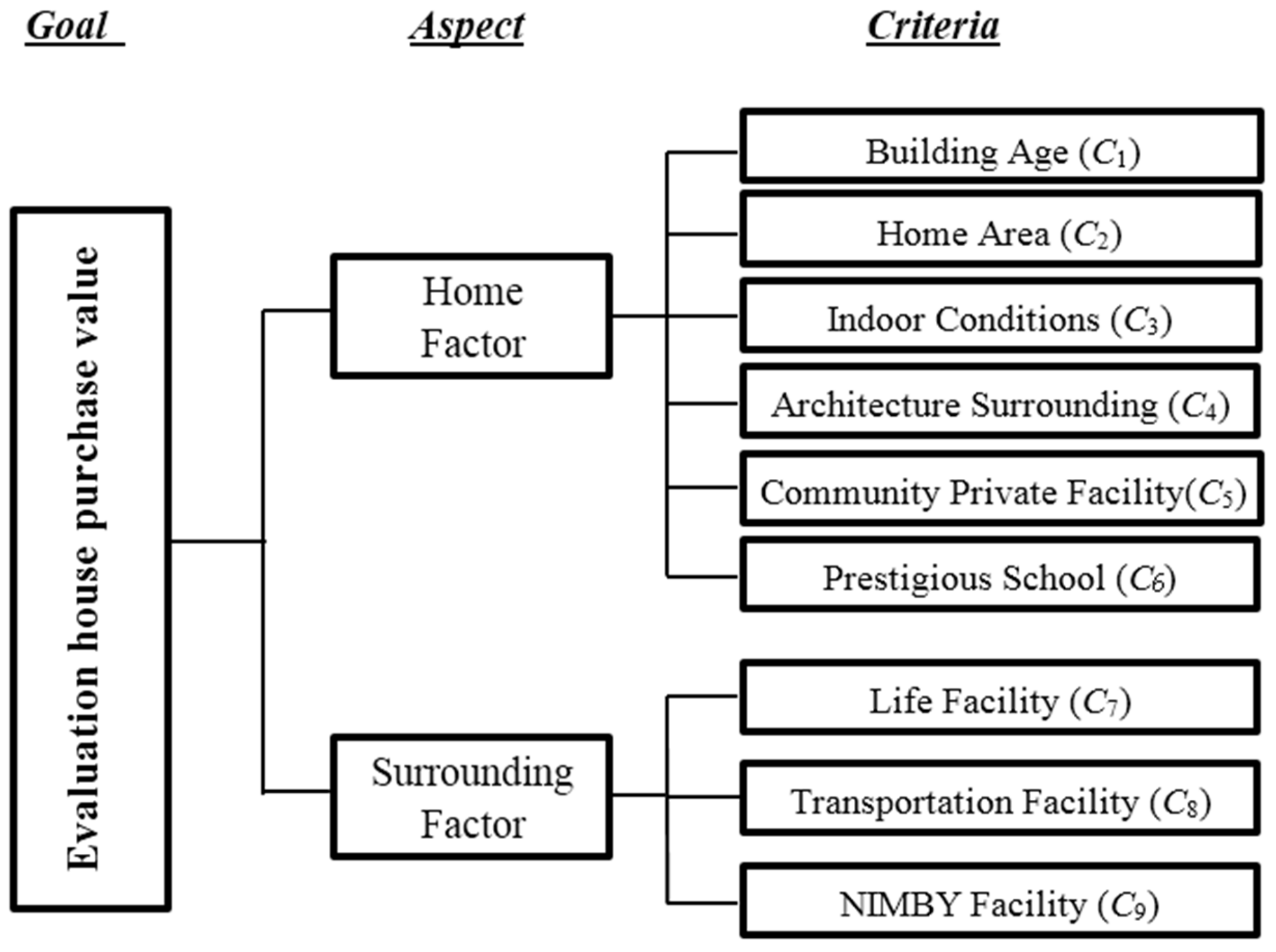
is the original decision matrix of scores for alternatives versus criteria.

The n criteria are ordinarily categorized as benefits or costs. A high value for a benefit criterion is preferable, while a low value for a cost criterion is preferable. Without a loss of generality, this study assumes that all criteria are a benefit type. We can transform a cost type criterion into a benefit type one via the following method. Let $w={\left\{w_1,w_2,\cdots ,w_n\right\}}^T$ be a criteria weight vector, where $w_j$ is the weight or the importance degree of criteria C_j, such that ${{\displaystyle \sum }}_{j=1}^n{w}_j=1$ and $0\le w_j\le 1$. Let $E={\left(e_1,e_2,\cdots ,e_n\right)}^T$ be an aspiration-level vector, where $e_j$ is the aspiration level of criteria C_j from the decision maker,$j\in N$. The decision maker can usually directly evaluate an aspiration-level criterion, according to the goal or the level that he/she desires to achieve. According to Fan et al. [10], “the aspiration level criterion can be set indirectly by the decision analyst according to the current asset position, the ideal points of the decision maker, or the values of historically similar situations”. Let $S={\left[s_{ij}\right]}_{m\times n}$ be a normalized matrix, where $s_{ij}$ is a normalized score. Our paper shall compare the alternative criteria $s_{ij}$ and aspiration level vector $E$.

The problem herein is to set up alternatives and select the most desirable ones from the finite set $P$ using normalized matrix $S$, aspiration level vector E, and criteria weight vector $w$. This study’s method is set up from the prospect theory to solve the above MCDM problem. Figure 2 shows the solution procedure for the method.

First, we define aspiration levels as reference points. Second, we calculate the gains and losses of alternatives based on perceived value differences between criteria and their reference points. Third, we measure the overall prospect values of alternatives using the value function and the simple additive weighting (SAW) method. This is also intuitive to decision makers [45]. Finally, we rank alternatives by comparing the obtained overall prospect values. The following section defines the procedures used to calculate gains, losses, and prospect values of alternatives, along with an algorithm for ranking alternatives.

3.2. The Utility Function

We define five utility functions based on real-world practices, as follows.

3.2.1. Crisp Utility Function

The form of the DM preference structure is “0–1”; that is, if the criteria performance meets or exceeds the DM aspiration level (in absolute numerical value or interval number), then the utility value is “1” and otherwise “0”.

3.2.2. Linear Utility Function

The DM utility value is “1” when the performance hits the aspiration level. The utility linearly drops when the performance deviates from the aspiration level.

3.2.3. S-shape Utility Function

Prelec [46] denoted that an S-shape implies that changes in probability have less impact as one moves away from the boundary of the probability interval, for instance, an initial sweep point seems more valuable than any additional ones. We set the DM utility value as “1” when the aspiration level is met, but the deviation from the aspiration level is used as a reference point.

3.2.4. Parabola Utility Function

The DM might be highly sensitive to changes in criteria. Here, the DM utility value remains “1” when the performance reaches the aspiration level, but sharply drops in a linear manner when the criteria performance deviates from the aspiration level. The parabola utility function can measure the utility value of attributes [12,47]. In the parabola utility function, we set parameter q. Usually, q = 2 is intuitive and practical for DMs in most scenarios [12].

3.2.5. Linguistic Utility Function

The performance of qualitative criteria might be presented by linguistic variables. Accordingly, DMs use linguistic variables to denote their aspirations with a fuzzy binary preference structure. The fuzzy logic is the same as that used for performance evaluations [12,48].

For example, an expert might regard “Middle” as the preferable indoor light in the optimal election. Here, “Middle” comes from linguistic term set S = {DL: Definitely Low, VL: Very Low, L: Low, M: Middle, H: High, VH: Very High, DH: Definitely High}. In this case, criteria performances and the DM aspiration are both in the form of linguistic variables. We process fuzzy linguistic information by first transforming linguistic variables into triangular fuzzy numbers while using

Table 2. Linguistic scales and their corresponding triangular fuzzy numbers.

Linguistic Variables and Semantic	Triangular Fuzzy Number
Definitely Low (DL)	(0, 0, 0.17)
Very Low (VL)	(0, 0.17, 0.33)
Low (L)	(0.17, 0.33, 0.5)
Middle (M)	(0.33, 0.5, 0.67)
High (H)	(0.5, 0.67, 0.83)
Very High (VH)	(0.67, 0.83, 1)
Definitely High (DH)	(0.83, 1, 1)

. The triplet (l, m, u) is known as triangular Fuzzy Number, where l represents smallest likely value, m the most possible value, and u the largest possible value of any fuzzy event. In the study, we assume that the five experts provide his/her preference information on some home factor (indoor conditions, architecture surrounding and community private facility) with regard to criteria by using a linguistic variable; we convert the linguistic variables to triangular fuzzy numbers.

Suppose that the criteria performance is x and that the DM’s aspiration level toward this criteria is e. We denote the DM’s utility function with aspirations as f(x|e).

Table 3. Possible cases’ utility function for the nine types.

Form	Types	Fuzzy Set Function	Case	Graphics
Binary	A	$f\left(x|e\right)=\left\{\begin{array}{cc}0,& x<a\\ 1,& x\ge a\end{array}\right.$	benefit
	B	$f\left(x|e\right)=\left\{\begin{array}{cc}1,& x<a\\ 0,& x\ge a\end{array}\right.$	cost
Line	C	$f\left(x|e\right)=\left\{\begin{array}{cc}0& x<a,\\ \left(\frac{x-a}{b-a} \right),& a\le x<b,\\ 1& b\le x.\end{array}\right.$	benefit
	D	$f\left(x|e\right)=\left\{\begin{array}{cc}1,& x<a,\\ \left(\frac{a-x}{b-a} \right),& a\le x<b,\\ 0,& b\le x.\end{array}\right.$	cost
S-shape	E	$f\left(x|e\right)=\left\{\begin{array}{cc}0,& x<a,\\ \frac{1}{2}+\frac{1}{2}\sin \left( \frac{\pi }{b-a}\right)\left(x-\frac{a+b}{2}\right)& a\le x<b,\\ 1,& b\le x.\end{array}\right.$	benefit
	F	$f\left(x|e\right)=\left\{\begin{array}{cc}1,& x<a,\\ \frac{1}{2}-\frac{1}{2}\sin \left( \frac{\pi }{b-a}\right)\left(x-\frac{a+b}{2}\right)& a\le x<b,\\ 0,& b\le x.\end{array}\right.$	cost
Parabola	G	$f\left(x|e\right)=\left\{\begin{array}{cc}0,& x<a,\\ 1-{\left(\frac{x-a}{b-a} \right)}^q,& a\le x<b,\\ 1,& b\le x.\end{array}\right.$	benefit
	H	$f\left(x|e\right)=\left\{\begin{array}{cc}1,& x<a,\\ {\left(\frac{x-a}{b-a} \right)}^q,& a\le x<b,\\ 0,& b\le x.\end{array}\right.$	cost
Linguistic	I	$f\left(x|e\right)=\left\{\begin{array}{cc}0,& u_a\le l_b,\\ \frac{l_a-u_b}{ (m_b-u_b)-(m_a-l_a)},& otherwise,\\ 1,& m_a\le m_b.\end{array}\right.$	Fuzzy

lists all of the utility functions under consideration.

3.3. Calculating the Gain and Loss Matrix

We take aspiration levels as reference points, in accordance with the prospect theory. We then measure the gains and losses of alternatives via differences in criteria values in comparison with reference points (aspiration levels). Since criteria values and aspiration levels are presented in five formats (Binary, Line, S-Shape, Parabola, and Linguistic), we can compare a criteria value in nine different ways (see Table 3). For each type, several different position relationships between $s_{ij}$ and $e_j$ are possible. The following remark pertains to the situation in which the criteria value and aspiration level are in the form of interval numbers.

Remark 1.

For normalized scores$s_{ij}$, let x be an arbitrary value that is a crisp or interval number. The value is taken to be a random variable with uniform distribution. For the aspiration level, if$e_j$is a crisp number, then$e_j=a ;$if$e_j$is an interval number, then$e_j=\left[a, b\right], a\le b$. The probability density function of x runs as follows.

• Crisp number

  $$f\left(x|e\right)=\left\{\begin{array}{cc}0,& x<a\\ 1,& x\ge a\end{array}\right.$$

  (1)

  where${{\displaystyle \int }}_a^{\infty }{f}_{ij}\left(x|e\right) d\left(x\right)=1$and$f_{ij}\left(x|e\right)\ge 0$for all$x\in \left[0, a\right]$.
• Interval number

  $$f\left(x|e\right)=\left\{\begin{array}{cc}0,& x<a,\\ \left(\frac{x-a}{b-a}\right),& a\le x<b,\\ 1& b\le x,\end{array}\right.$$

  (2)

  where${{\displaystyle \int }}_a^b{f}_{ij}\left(x|e\right) d\left(x\right)=1$and$f_{ij}\left(x|e\right)\ge 0$for all$x\in \left[a, b\right]$.
• Fuzzy set number

  $$f\left(x|e\right)=\left\{\begin{array}{cc}0,& u_a\le l_b,\\ \frac{l_a-u_b}{ (m_b-u_b)-(m_a-l_a)},& otherwise,\\ 1,& m_a\le m_b, \end{array}\right.$$

  (3)

  where${{\displaystyle \int }}_a^b{f}_{ij}\left(x|e\right) d\left(x\right)=1$and$f_{ij}\left(x|e\right)\ge 0$for all$x\in \left[a, b\right]$.

We calculate the gain and loss of each alternative relative to the negative ideal solution and the positive ideal solution. First, we should compare the criteria values of alternatives $s_{ij}$ by pairs. Second, we respectively express the gain and loss of alternative A_i relative to alternative concerning criteria C_j, $G_{ij}$, and $L_{ij}$, as:

$$G_{ij}=\frac{s_{ij}-min\left(s_{ij}\right)}{max\left(s_{ij}\right)-min\left(s_{ij}\right) }$$

(4)

$$L_{ij}=\frac{s_{ij}-max\left(s_{ij}\right)}{max\left(s_{ij}\right)-min\left(s_{ij}\right)}$$

(5)

Furthermore, we set up a gain matrix $G={\left[G_{ij}\right]}_{m\times n}$ and a loss matrix $L={\left[L_{ij}\right]}_{m\times n},$ respectively.

3.4. Calculating the Prospect Values and Ranking of Alternatives

We normalize matrices $G$ and L through Equations (4) and (5), respectively, to transform the gains and losses into comparable values because gains or losses concerning different criteria are generally incommensurate. To achieve this, every element in matrix $G={\left[G_{ij}\right]}_{m\times n}$ or $L={\left[L_{ij}\right]}_{m\times n}$ must be normalized to a corresponding element in matrix $G^{*}={\left[G_{ij}^{*}\right]}_{\times n}$ or $L^{*}={\left[L_{ij}^{*}\right]}_{m\times n}$ while using the following formula:

$$G_{ij}^{*}=\frac{G_{ij}}{max\left(G_{ij}\right)}, i\in M, j\in N.$$

(6)

$$L_{ij}^{*}=\frac{L_{ij}}{max\left(L_{ij}\right)}, i\in M, j\in N.$$

(7)

Thus, based on the value function, the prospect value of alternative $A_i$ with respect to criteria $j , {\nu }_{ij}$ is:

$${\nu }_{ij}={\left(G_{ij}^{*}\right)}^{\alpha }+\left[-\lambda {\left(-L_{ij}^{*}\right)}^{\beta }\right],i\in M,j\in N,$$

(8)

where α and β are estimable parameters for the concavity and convexity of the value function and they represent the decision maker’s risk attitudes for gains and losses, respectively. The literature widely regards $0\le \alpha , \beta \le 1$, so as to be consistent with the property of diminishing sensitivity. As α decreases, the risk aversion in the gain domain increases. Similarly, when β decreases, risk-seeking in the loss domain increases. We note that $\lambda$ is the parameter for loss aversion, and the assumption is $\lambda$ > 1, which means that the decision maker is sensitive to losses and gains. As $\lambda$ increases, the sensitivity to losses becomes higher than the sensitivity to gains.

Tversky and Kahneman [24] conducted several experiments to obtain the values of α, β, and $\lambda$. Their experiments use the linear regression procedure to estimate the parameters, finding that the median values of α and β are both 0.88, and that the value of $\lambda$ is 2.25. These parameter values are considered to be appropriate for describing most decision makers’ behavior. Other scholars obtained the same values for the parameters through experiments [10,49,50]. Therefore, we also apply the values from Tversky and Kahneman [24]; i.e., α = β = 0.88 and $\lambda$ = 2.25. The simple additive weighting (SAW) method calculates the overall prospective value of the alternatives (i.e., [45,51]). A prospect value matrix ${\nu }^{*}$ is constructed using Equation (9).

$${\nu }^{*}=w_j\times {\left[{\nu }_{ij}\right]}_{m\times n}, i\in M,j\in N.$$

(9)

After calculating the diverse partial matrices of dominance (one for each criterion), we obtain the final dominance matrix of the general element ${\nu }^{*}$ using Equation (9) to sum the elements of the diverse matrices.

$${\mu }_i=\frac{{{\displaystyle \sum }}_{j=1}^m{\nu }_{ij}^{*}-min{{\displaystyle \sum }}_{j=1}^m{\nu }_{ij}^{*}}{max{{\displaystyle \sum }}_{j=1}^m{\nu }_{ij}^{*}-min{{\displaystyle \sum }}_{j=1}^m{\nu }_{ij}^{*}}$$

(10)

The term ${\mu }_i$, denoted by the global measures obtained by Equation (10), permits a complete ranking of all alternatives. The rank of every alternative originates from the ordering of the respective values of the two options. As a final step of the developed methodology, global measurements are available, since parameter values in real-life applications originate from estimations with variable reliability (weighting factors, thresholds, criteria qualitative values, etc.). Clearly, as ${\mu }_i$ increases, the corresponding alternative $A_i$ rises. Therefore, we rank all alternatives and select desirable alternatives based on the descending order of the overall prospect values of all alternatives. The procedure for solving the MCDM problems by considering the aspiration level can be summarized, as follows.

Step 1.

Construct an evaluation matrix of alternatives versus criteria in Table 1.

Step 2.

Use the calculation formulae in Table 3 to rank the quality and quantity criteria preferences.

Step 3.

Set up gain matrix $G={\left[G_{ij}\right]}_{m\times n}$ and loss matrix $L={\left[L_{ij}\right]}_{m\times n}$ using Equations (4) and (5), respectively.

Step 4.

Build normalized matrices $G^{*}={\left[G_{ij}^{*}\right]}_{m\times n}$ and $L^{*}={\left[L_{ij}^{*}\right]}_{m\times n}$ while using Equations (6) and (7), respectively.

Step 5.

Write up prospect value matrix ${\nu }^{*}={\left[{\nu }_{ij}^{*}\right]}_{m\times n}$ using Equations (8) and (9).

Step 6.

Calculate the overall prospect value of each alternative using Equation (10).

Step 7.

Determine the ranking order of alternatives according to the obtained overall prospect values.

4. Empirical Analysis

This section presents an example of an application of the proposed method. From the aspiration utility functions depicted in Section 3.3, the experts identified the utility function types for setting up the decision criteria (see

Table 4. Definitions of decision criteria and utility function types.

Factor	Criteria	Definition	Measure
Home Attribute	Building Age (C1)	--	A quantitative criterion for measuring the age of a home. (Unit: year)
	Home Area (C2)	The area provides the household usage living space.	A quantitative criterion for measuring the indoor space (Unit: square meter).
	Indoor Conditions (C3)	The indoor conditions may provide a comfortable sense and a healthy environment.	The indoor conditions are assessed by the DMs through their subjective judgment and prediction (density). The indoor conditions include sunlight in front, natural ventilation, lighting, view, and so on.
	Architecture Surrounding (C4)	The outdoor layout of the architecture surrounding as proposed by the architects.	The ratio of the homes in surrounding environments is assessed by the DMs through their subjective judgement and prediction (density). The architecture surrounding is categorized as against a hill, surrounded by trees, a waterfront view, path in front, open space in front, open view in front, and so on.
	Community Private Facility (C5)	The community’s private facilities provide a household with usable facilities and the feeling of safety.	Community private facilities include security management, parking lot, gym, salon, swimming pool, lobby, and so on.
	Prestigious School (C6)	Homes within a prestigious school district can influence owners to give a better education to their children and improve their relative position.	If the home is near a prestigious school area, then evaluation is “yes” and otherwise “no” (density). A prestigious school includes elementary school, junior school, high school, university, and so on.
Surrounding Attribute	Life Facility (C7)	Amenities and facilities near the home provide a household with the conveniences of daily life activities.	Daily life facilities include convenience stores, banks, post office, sports center, supermarkets, department stores, traditional markets, parks or green areas, and so on.
	Transportation Facility (C8)	Transportation facilities nearby a home may reduce commuting time and costs.	Transportation facilities include Metro Rapid Transit (MRT) stations, bus stations, highway entrance, etc.
	NIMBY Facility (C9)	Nearby undesirable facilities/ NIMBY facilities can worry homeowners and impact human health (noise).	NIMBY facilities include power stations, viaducts, petrol stations, shrines, temples, crematoriums, cemeteries, etc.

).

Table 5. Original decision matrix.

Criteria	C1	C2	C3	C4	C5	C6	C7	C8	C9
Utility function Type	D	C	I	I	I	A	E	E	F
Aspiration level	[5, 30]	[60, 100]	H	H	M	2	[3, 6]	[2, 5]	[0, 1]
Alternative
A1	33	97.4	DH	L	L	0	2	2	0
A2	12	95.5	H	M	M	1	5	2	0
A3	25	76	M	H	VL	2	3	2	0
A4	6	84.7	M	L	VH	3	4	3	0
A5	12	67	L	VH	H	1	4	4	1
A6	16	83.1	M	H	M	2	5	4	1
A7	35	98.7	H	VL	VL	1	6	3	2
A8	36	84.5	VH	M	VL	0	5	3	0
A9	32	97.3	VH	M	L	3	7	4	0
A10	22	94.1	DH	VH	M	2	4	2	0
A11	31	84.7	M	M	L	2	3	2	1
A12	15	107	DH	M	DH	3	5	3	0
A13	25	99.1	M	M	M	2	6	2	1
A14	21	84.7	L	H	H	0	8	2	0
A15	5	92.6	M	L	DH	4	3	3	0

lists the original decision matrix of quantitative and qualitative criteria.

Site-specific data were used in tests before modeling the survey data that were obtained from the scenarios. Nine types of aspiration utility functions $f\left(x|e\right)$ (see Table 3) were applied when using the data to assess the influence of site-specific characteristics and home criteria. The analytical results showed that data from the two stations are independent of the site and can be combined to create a single dataset.

Table 6. Scores for the normalized alternatives against the criteria.

Criteria	C1	C2	C3	C4	C5	C6	C7	C8	C9
A1	0	0.935	1	0	0.50	0	0	0	1
A2	0.72	0.8875	1	0.50	1	0	0.75	0	1
A3	0.2	0.4	0.50	1	0	1	0	0	1
A4	0.96	0.6175	0.50	0	1	1	0.25	0.25	1
A5	0.72	0.175	0	1	1	0	0.25	0.75	0.25
A6	0.56	0.5775	0.50	1	1	1	0.75	0.75	0.25
A7	0	0.9675	1	0	0	0	1	0.25	0
A8	0	0.6125	1	0.50	0	0	0.75	0.25	1
A9	0	0.9325	1	0.50	0.50	1	1	0.75	1
A10	0.32	0.8525	1	1	1	1	0.25	0	1
A11	0	0.6175	0.50	0.50	0.50	1	0	0	0.25
A12	0.6	1	1	0.50	1	1	0.75	0.25	1
A13	0.2	0.9775	0.50	0.50	1	1	1	0	0.25
A14	0.36	0.6175	0	1	1	0	1	0	1
A15	1	0.815	0.50	0	1	1	0	0.25	1

lists the scores for the normalized alternatives against the criteria.

In accordance with the importance given to the criteria used to evaluate the properties in the study, their respective weights were defined by the decision-makers through direct evaluation. The direct valuation was performed by assigning each criterion a number from 1 to 5 (‘least important’ to ‘most important’, respectively). The weights were assigned by the decision-makers. The decision-maker was the realtor in this example.

Table 7. Calculation of decision maker preference weights.

Criterion	Description	Assigned Weights	Criteria Weights
C1	Building Age	4	0.13
C2	House Area	5	0.16
C3	Indoor Conditions	3	0.09
C4	Architecture Surrounding	2	0.06
C5	Community Private Facility	3	0.09
C6	Prestigious School	1	0.03
C7	Life Facility	5	0.16
C8	Transportation Facility	5	0.16
C9	NIMBY Facility	4	0.13

presents the information.

Using Equations (6) and (7), we can obtain the matrices $G^{*}$ and $L^{*}$, respectively.

$$G^{*}=\left[\begin{array}{ccc}\begin{array}{ccc}0& 0.76& 1\\ 0.72& 0.72& 1\\ 0.2& 0.23& 0.5\end{array}& \begin{array}{ccc}0& 0.5& 0\\ 0.5& 1& 0\\ 1& 0& 1\end{array}& \begin{array}{ccc}0& 0& 1\\ 0.75& 0& 1\\ 0& 0& 1\end{array}\\ \begin{array}{ccc}0.96& 0.45& 0.5\\ 0.72& 0& 0\\ 0.56& 0.41& 0.5\end{array}& \begin{array}{ccc}0& 1& 1\\ 1& 1& 0\\ 1& 1& 1\end{array}& \begin{array}{ccc}0.25& 0.25& 1\\ 0.25& 0.75& 0.25\\ 0.75& 0.75& 0.25\end{array}\\ \begin{array}{ccc}0& 0.79& 1\\ 0& 0.44& 1\\ 0& 0.76& 1\end{array}& \begin{array}{ccc}0& 0& 0\\ 0.5& 0& 0\\ 0.5& 0.5& 1\end{array}& \begin{array}{ccc}1& 0.25& 0\\ 0.75& 0.25& 1\\ 1& 0.75& 1\end{array}\\ \begin{array}{ccc}0.32& 0.68& 1\\ 0& 0.44& 0.5\\ 0.6& 0.83& 1\end{array}& \begin{array}{ccc}1& 1& 1\\ 0.5& 0.5& 1\\ 0.5& 1& 1\end{array}& \begin{array}{ccc}0.25& 0& 1\\ 0& 0& 0.25\\ 0.75& 0.25& 1\end{array}\\ \begin{array}{ccc}0.2& 0.80& 0.5\\ 0.36& 0.44& 0\\ 1& 0.64& 0.5\end{array}& \begin{array}{ccc}0.5& 1& 1\\ 1& 1& 0\\ 0& 1& 1\end{array}& \begin{array}{ccc}1& 0& 0.25\\ 1& 0& 1\\ 0& 0.25& 1\end{array}\end{array}\right]$$

$$L^{*}=\left[\begin{array}{ccc}\begin{array}{ccc}-1& -0.065& 0\\ -0.28& -0.112& 0\\ -0.8& -0.6& -0.5\end{array}& \begin{array}{ccc}-1& -0.5& -1\\ -0.5& 0& -1\\ 0& -1& 0\end{array}& \begin{array}{ccc}-1& -0.75& 0\\ -0.25& -0.75& 0\\ -1& -0.75& 0\end{array}\\ \begin{array}{ccc}-0.04& -0.382& -0.5\\ -0.28& -0.825& -1\\ -0.44& -0.422& -0.5\end{array}& \begin{array}{ccc}-1& 0& 0\\ 0& 0& -1\\ 0& 0& 0\end{array}& \begin{array}{ccc}-0.75& -0.5& 0\\ -0.75& 0& -0.75\\ -0.25& 0& -0.75\end{array}\\ \begin{array}{ccc}-1& -0.032& 0\\ -1& -0.387& 0\\ -1& -0.067& 0\end{array}& \begin{array}{ccc}0& -1& -1\\ 0& -0.5& -1\\ 0& -0.5& -0.5\end{array}& \begin{array}{ccc}0& -0.5& -1\\ -0.25& 0& 0\\ 0& -0.75& 0\end{array}\\ \begin{array}{ccc}-0.68& -0.147& 0\\ -1& -0.382& -0.5\\ -0.4& 0& 0\end{array}& \begin{array}{ccc}0& 0& 0\\ -0.5& -0.5& 0\\ -0.5& 0& 0\end{array}& \begin{array}{ccc}-0.75& -0.75& 0\\ -1& -0.5& -0.75\\ -0.25& -0.75& 0\end{array}\\ \begin{array}{ccc}-0.8& -0.022& -0.5\\ -0.64& -0.382& -1\\ 0& -0.185& -0.5\end{array}& \begin{array}{ccc}-0.5& 0& 0\\ 0& 0& -1\\ -1& 0& 0\end{array}& \begin{array}{ccc}0& 0& -0.75\\ 0& -0.75& 0\\ -1& -0.5& 0\end{array}\end{array}\right]$$

According to the experimental results reported by Tversky and Kahneman [24], $\alpha =\beta =0.88,$ and $\lambda =2.25$ in Equation (8). Thus, the prospect value matrix (or the resulting prospect value matrix) is obtained, as follows:

$${\nu }^{*}=\left[\begin{array}{ccc}\begin{array}{ccc}-0.281& 0.091& 0.094\\ 0.002& 0.065& 0.094\\ -0.201& -0.182& -0.064\end{array}& \begin{array}{ccc}-0.141& -0.064& -0.070\\ -0.042& 0.094& -0.070\\ 0.063& -0.211& 0.031\end{array}& \begin{array}{ccc}-0.352& -0.273& 0.125\\ 0.018& -0.273& 0.125\\ -0.352& -0.273& 0.125\end{array}\\ \begin{array}{ccc}0.104& -0.075& -0.064\\ 0.002& -0.297& -0.211\\ -0.062& -0.095& -0.064\end{array}& \begin{array}{ccc}-0.141& 0.094& 0.031\\ 0.063& 0.094& -0.070\\ 0.063& 0.094& 0.031\end{array}& \begin{array}{ccc}-0.227& -0.145& 0.125\\ -0.227& 0.121& -0.181\\ 0.018& 0.121& -0.181\end{array}\\ \begin{array}{ccc}-0.281& 0.110& 0.094\\ -0.281& -0.077& 0.094\\ -0.281& 0.090& 0.094\end{array}& \begin{array}{ccc}-0.141& -0.211& -0.070\\ -0.042& -0.211& -0.070\\ -0.042& -0.064& 0.031\end{array}& \begin{array}{ccc}0.156& -0.145& -0.281\\ 0.018& -0.145& 0.125\\ 0.156& 0.121& 0.125\end{array}\\ \begin{array}{ccc}-0.154& 0.046& 0.094\\ -0.281& -0.075& -0.064\\ -0.046& 0.132& 0.094\end{array}& \begin{array}{ccc}0.063& 0.094& 0.031\\ -0.042& -0.064& 0.031\\ -0.042& 0.094& 0.031\end{array}& \begin{array}{ccc}-0.227& -0.273& 0.125\\ -0.352& -0.273& -0.181\\ 0.018& -0.145& 0.125\end{array}\\ \begin{array}{ccc}-0.201& 0.116& -0.064\\ -0.139& -0.075& -0.211\\ 0.125& 0.026& -0.064\end{array}& \begin{array}{ccc}-0.042& 0.094& 0.031\\ 0.063& 0.094& -0.070\\ -0.141& 0.094& 0.031\end{array}& \begin{array}{ccc}0.156& -0.273& 0.181\\ 0.156& -0.273& 0.125\\ -0.352& -0.154& 0.125\end{array}\end{array}\right]$$

5. Results and Discussion

Based on the prospect value matrix ${\nu }^{*}$, Equation (10) were used to realize the overall prospect value of each alternative after weighting user preferences.

Table 8. Final evaluation performance of ranking.

Alternative	A1	A2	A3	A4	A5	A6	A7	A8	A9	A10	A11	A12	A13	A14	A15
Performance	0.275	0.840	0.152	0.643	0.380	0.785	0.340	0.455	0.981	0.704	0.0	1.0	0.600	0.622	0.641
Ranking	13	3	14	6	11	4	12	10	2	5	15	1	9	8	7
Price (million NT$)	13.5	11.17	12.43	10.15	17.84	18.69	12.5	13.52	13.6	17.82	9.6	19.8	16	11.84	18.35

presents each alternative performance and price. The table ranks 15 candidates in order of home performance. The final evaluation suggests that alternative A₁₂ is desirable while A₁₁ is undesirable. While performance and property prices have distinct characteristics, they are not dichotomized as clearly, as suggested by this discussion.

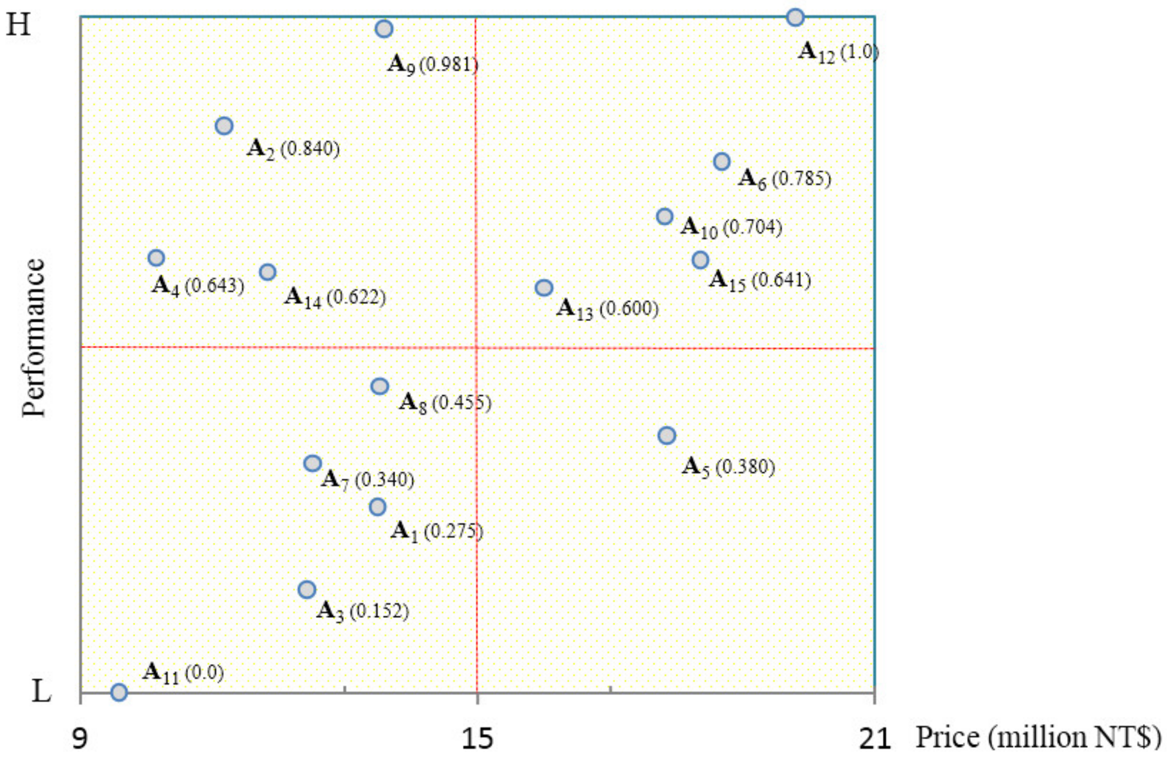
Figure 3 shows a ‘two-dimension’ sensitivity analysis that links home prices to the performance map. The transversely priced component is based on the alternative asking price, and the longitudinal performance components are based on the aspiration level score. The figure also presents each alternative in terms of performance and price in order to fully exploit the inherent four-quadrant alternative choice capability. Therefore, each alternative is considered in terms of the performance at the aspiration level to reference the list price. A general method of obtaining a four-quadrant dimensional alternative is described. We consider the home price performance state transformation when a high home price results from a high numerical performance objective for an intuitive understanding of the method and principle of a four-quadrant phase.

When comparing the seller’s asking price and the estimation performance, the home price profiles can be divided into four independent quadrants. The strengthened component is mainly concentrated on the performance and price of the optical axes x and y, which is an effective method of organizing the decision maker’s priorities. Figure 3 shows that quadrant 1 is opposite to quadrant 3 if its performance is superior and if it sells at a higher price. There are four quadrants organized by home price and performance, as we can see from the grid below. The alternative’s price is affected by home performance in that higher performance has a higher asking price (quadrant 1) and vice versa (quadrant 3). Notably, quadrant 2 denotes that the home value is more than its worth, and opposite to quadrant 4 is the worthless area.

The optimal attainment and the target value are also set for each home buyer. The broker might recommend the buyer to select a different home based on considerations of affordability: for example, in a low price area, the broker may recommend quadrant 2 area alternatives, such as optimal homes A₄, A₂, A₉, and A₁₄. In an area with high home prices, the broker might also recommend an optimal home in quadrant 1 area alternative A₁₂. For desirable property A₁₂ has both the highest performance and the highest total price.

6. Conclusions

This empirical study finds that the proposed approach herein based on buyer preferences identifies better candidate homes as compared to the conventional sorting approach. Alternative outcomes can be determined by identifying and analyzing the best case and worst-case scenarios. The results of empirical analyses indicate that the pricing strategy improves the brokerage intermediation effects. Brokers can then provide recommendations on a suitable price, make decisions over negotiation strategies to reach an agreement, and settle on an acceptable price. To examine accessibility, this study collected information regarding nine different urban amenities to acquire a complete dataset of service amenities. The homebuyer can then consider the quality and affordability of a home.

When used for property evaluation, both of the approaches can assist professionals in the real estate market by clearly evaluating alternatives in relation to the criteria defined by the experts. The purchasing evaluation of a property is among the most important tasks of real estate professionals.

We also analyze the alternatives by using both aspiration-level and the prospect theory to ranks orders for extreme values. Of note is that the values are quite close and in agreement with the expectations of the experts. Through the formulation, the model makes it easier to resolve conflicts between criteria. It is necessary to not be concerned about the performance of another criterion in order to achieve good performance in a determined criterion of the analysis.

The presented analysis and solution obtained by aspiration-level MCDM accurately reflect the preferences of the agents. Consequently, we conclude that both methods enable effective property evaluation. As new properties are added to the portfolio of a realtor, either of the two methods must be performed again in order to account for the characteristics of the new properties. According to the realtors, the method is effective for evaluating residential properties, especially when taking the extreme difficulties in assigning home values to all evaluation criteria into account. Given new evaluation scenarios and with a new set of evaluation criteria, new applications of the multicriteria analysis will have to be performed. Different scenarios obtain different changes in estimated home values, even for properties whose values have been defined previously. Further studies are needed in order to quantify the monetary consequences that are associated with each criterion.