Free Vibration Analysis of Axially Functionally Graded (AFG) Cantilever Columns of a Regular Polygon Cross-Section with Constant Volume

Abstract

This paper deals with the transverse free vibration of axially functionally graded (AFG) cantilever columns under the influence of axial compressive load. The columns possessing a regular polygon in their cross-section are tapered and their material properties vary along the axis of the column. An emphasis is placed on the columns with constant volume for admissible geometries and materials. The governing differential equation of the problem is derived and solved using the direct integral approach in conjunction with the determinant search technique. The obtained results are in good agreement with those in the available literature and computed by finite element analysis. Numerical examples for the natural frequency and mode shape of the columns are presented to investigate the effects of parameters related to geometrical nonuniformity and material inhomogeneity.

1. Introduction

In a variety of structural engineering applications, columns are often built as one of the most important main components by which axial compressive forces, one of the main types of external loading, are supported [1]. As a result, over the past few decades, many researchers have devoted a lot of effort to improving the analysis of column structure systems. After the concept of functionally graded material (FGM) was established in 1984 by material scientists in Japan, recently, FGM is usually composited from ceramic and metallic materials, because these composites enhance the advantages of the materials, such as stronger mechanical performance, as well as better thermal resistance [2]. Therefore, FGM has been successfully applied for various engineering applications, such as aerospace, precision machinery, and biomedical structures. Due to the benefits of space utilization, esthetics, safety, optimization, and economy, tapered components are typically used in engineering practices [3]. In particular, taper elements behave differently from the uniform ones because of the variation of the cross-section along the axial coordinate yields effective stress distributions and a strong coupling between the stress resultants. This concept is important for optimizing the structural members and reducing the self-weight. Thus, by adopting tapered components, safe and economical designs are achieved.

In this respect, much research has been undertaken on the above-mentioned subject that deals with functionally graded cantilever columns. Generally, FGMs are divided into two types: laterally functionally graded material (LFGM) in which the mechanical properties, i.e., the Young’s modulus and mass density, are composited laterally to the axial coordinate; and axially functionally graded material (AFGM) in which its properties are composited axially along the coordinate. In this study, AFGM is a major concern for analyzing the free vibration of the cantilever columns.

For the free vibration problems in this subject, the mathematical models include the inertia forces, which are treated as the static quantities. The following references and their citations include the mathematical models and historical reviews of this subject. The typical studies on free vibration of AFG columns are briefly reviewed here in chronological order: Akgoz and Civalek [3] studied natural frequencies of a linearly tapered microbeam based on the modified couple stress theory; Calio and Elishakoff [4] investigated the closed-form solutions of natural frequency for a simply supported beam-column with an elastically guided end condition at one end, where the trigonometric functions of the Young’s modulus in the mathematical formulation were considered; Li [5] studied the static and dynamic behaviors of a prismatic beam, including the rotatory inertia and shear deformation; Singh and Li [6] studied critical buckling loads of a cantilever column with a piecewise element, restrained by the elastic foundation; Huang and Li [7] researched a new approach for the free vibration of tapered beams with simply supported, both clamped, clamped-pinned, and cantilevered end conditions, respectively, where the Fredholm integral equations were used in the mathematical formulations; Shahba et al. [8] investigated the free vibration and stability of a non-prismatic column with classical and non-classical boundary conditions; Shahba and Rajasekaran [9] studied the free vibration and stability of tapered beams, in which governing equations for the free vibration and buckling were solved by the differential quadrature element method (DQEM); Kukla and Rychlewska [10] dealt with beams with both ends fixed, which were fabricated from two different FGMs for analyzing free vibration; Yilmaz et al. [11] investigated the buckling loads of non-prismatic columns restrained by the elastic foundation using the differential quadrature method (DQM); Chandran and Rajendran [12] studied closed-form solutions of the buckling load of a prismatic cantilever column using the principle of conservation energy; Shafiei et al. [13] studied non-linear vibrations of a linearly tapered microbeam with a square cross-section, where the governing equations were solved by the differential quadrature method (DQM); Ranganathan et al. [14] studied the buckling of slender columns that determined the buckling loads by the linear perturbation method together with the Rayleigh-Ritz method and investigated the maximum buckling loads under the same average mean Young’s modulus; Elishakoff et al. [15] studied the buckling and vibrations of a column sharing Duncan’s mode shapes and assuming a fifth order polynomial; Rezaiee and Masoodi [16] investigated closed-form solutions of the natural frequencies and buckling loads of tapered beam-columns supported by semi-rigid connections; and Lee and Lee [17] studied the free vibration and buckling of tapered cantilever columns with square and circular cross-sections. As discussed above, FG materials developed in 1984 are of particular interest in dealing with the free vibration of FG columns.

This paper presents a unique numerical approach for analyzing the free vibration of AFG cantilever columns. In terms of geometry, the column is tapered, the cross-sectional shape is a regular polygon, and the volume of the columns is constant. In the literature, the scope of this topic has not yet been covered. This paper consists of the following contents: Section 2 describes the mathematical model of the problem. By using the equilibrium of free body diagram of the column element subjected to the transverse and rotatory inertia loadings, the differential equation governing the mode shape of vibrating columns is derived with its boundary conditions. A variable function for the Young’s modulus of AFGMs is adopted as a linear function, and in terms of the column geometry, three taper functions are selected as the linear, parabolic, and sinusoidal taper. Section 3 shows the solution methods to the problems of this study. To calculate natural frequencies along with their corresponding mode shapes, the governing differential equation is solved by the direct integral method enhanced by the determinant search method. For the verification purpose, the predicted natural frequencies are compared with those obtained by the general-purpose software ADINA and the references. Section 4 deals with the numerical experiments and provides a discussion. The effects of the material and geometrical properties of AFG cantilever columns on free vibration behaviors are extensively discussed. Section 5 summarizes this study and suggests areas for further study.

2. Mathematical Model

Shown in Figure 1a is an AFG cantilever column with a length $l$ and a volume $V$. From a geometrical point of view, the column is tapered, the cross-sectional shape is a regular polygon with an integer side number $k\left(\ge 3\right)$, as shown in Figure 1c, and the column volume $V$ is constant. The axial coordinate $x$ is zero at the clamped end, and the circumradius, area, and second moment of the regular polygonal cross-section are denoted by $r$, $A$, and $I$, respectively. The Young’s modulus and mass density are represented by $E$ and $\rho$, and the flexural rigidity is denoted by $R_f\left(=EI\right)$. At the clamped end ($x=0$), $r$, $E$, and $\rho$ are denoted by $r_c$, $E_c$, and ${\rho }_c$. At the free end ($x=l$), $r$, $E$, and $\rho$ are denoted by $r_f$, $E_f$,AF and ${\rho }_f$. The column is externally subjected to an axial compressive load $P$ less than the buckling load $B$ at the free end.

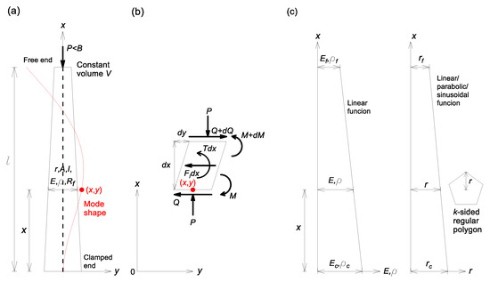
Figure 1. (a) Schematic view of an axially functionally graded (AFG) cantilever column with constant volume; (b) free body diagram of the column element; (c) variations of Young’s modulus (and mass density) and circumradius of the regular polygon.

When the column vibrates, the undeformed column axis depicted by the straight dashed line elastically deforms the mode shape depicted by the solid line in Figure 1a, defined in Cartesian coordinates $\left(x,y\right)$. The cross-section of the deformed column is subjected to the dynamic shear force $Q$ and bending moment $M$, as well as the axial force $P$. The column element shown in Figure 1b is loaded to the transverse inertia force $F_I$ and the rotatory inertia couple $T$, since the column has mass. In this study, the free vibration is a harmonic motion in which each dynamic coordinate is proportional to sin$\left({\omega }_{i}t\right)$. For example, $y_{x,t}=y_x\sin \left({\omega }_{i}t\right)$ where $y_x\left(=y\right)$ is the transverse deflection, ${\omega }_i$ is the angular frequency in motion where the dynamic co0 $i\left(=1,2,3,\cdots \right)$ is the mode number, and $t$ is the time.

Using the equations of ${\displaystyle \sum }{F}_y=0$ and ${\displaystyle \sum }{M}_{\left(x,y\right)}=0$ established from the free body diagram shown in Figure 1b, the equations of the dynamic equilibrium are obtained as

$${\displaystyle \sum }{F}_y=\left(Q+dQ\right)-Q-F_{I}dx=0: \frac{dQ}{dx}-F_I=0$$

(1)

$${\displaystyle \sum }{M}_{\left(x,y\right)}=\left(Q+dQ\right)dx+Pdy-\left(M+dM\right)+M-Tdx=0: \frac{dM}{dx}-Q-P\frac{dy}{dx}+T=0$$

(2)

From Equation (2), the first derivative $dM/dx$ is re-arranged as

$$\frac{dM}{dx}=P\frac{dy}{dx}+Q-T$$

(3)

Combining the second derivative $d^{2}M/d{x}^2$ obtained from Equation (3) and $dQ/dx=F_I$ in Equation (1) yields

$$\frac{d^{2}M}{d{x}^2}=P\frac{d^{2}y}{d{x}^2}-\frac{dT}{dx}+F_I$$

(4)

The bending moment $M$, transverse inertia force $F_I$, and rotatory inertia couple $T$ are expressed as [18,19]

$$M=-EI\frac{d^{2}y}{d{x}^2}=-R_f\frac{d^{2}y}{d{x}^2}$$

(5)

$$F_I=-\rho A{\omega }_i^{2}y$$

(6)

$$T=-R\rho I{\omega }_i^2\frac{dy}{dx}$$

(7)

where the rotatory inertia index $R$ is defined as

$$R=0, \mathrm{if} \mathrm{rotatory} \mathrm{inertia} \mathrm{couple} \mathrm{is} \mathrm{excluded}; R=1, \mathrm{if} \mathrm{included}.$$

(8)

From Equation (7), the first derivative $dT/dx$ is obtained as

$$\frac{dT}{dx}=-R{\omega }_i^2\left[\rho I\frac{d^{2}y}{d{x}^2}+\left(\frac{d\rho }{dx}I+\rho \frac{dI}{dx}\right)\frac{dy}{dx}\right]$$

(9)

Substituting Equations (6) and (9) into Equation (4) yields Equation (10), and from Equation (5), the second derivative $d^{2}M/d{x}^2$ is obtained as Equation (11):

$$\frac{d^{2}M}{d{x}^2}=P\frac{d^{2}y}{d{x}^2}+R{\omega }_i^2\left[\rho I\frac{d^{2}y}{d{x}^2}+\left(\frac{d\rho }{dx}I+\rho \frac{dI}{dx}\right)\frac{dy}{dx}\right]-\rho A{\omega }_i^{2}y$$

(10)

$$\frac{d^{2}M}{d{x}^2}=-R_f\frac{d^{4}y}{d{x}^4}-2\frac{d{R}_f}{dx}\frac{d^{3}y}{d{x}^3}-\frac{d^2{R}_f}{d{x}^2}\frac{d^{2}y}{d{x}^2}$$

(11)

Using Equations (10) and (11) and re-arranging against $d^{4}y/d{x}^4$ yields the following equation, or

$$\frac{d^{4}y}{d{x}^4}=-\frac{2}{R_f}\frac{d{R}_f}{dx}\frac{d^{3}y}{d{x}^3}-\frac{1}{R_f}\left(P+\frac{d^2{R}_f}{d{x}^2}\right)\frac{d^{2}y}{d{x}^2}-R{\omega }_i^2\left[\rho I\frac{d^{2}y}{d{x}^2}+\left(\frac{d\rho }{dx}I+\rho \frac{dI}{dx}\right)\frac{dy}{dx}\right]+{\omega }_i^2\frac{\rho A}{R_f}y$$

(12)

Now consider the boundary conditions of the column ends ($x=0$ and $x=l$). At the clamped end ($x=0$), the deflection $y$ and the rotation $dy/dx$ are zero:

$$y=0; \frac{dy}{dx}=0$$

(13)

At the free end ($x=l$), the bending moment $M$ in Equation (5) and the shear force $Q$ in Equation (3) together with Equations (5) and (7) are zero, that is

$$\frac{d^{2}y}{d{x}^2}=0; \frac{d^{3}y}{d{x}^3}+\frac{1}{R_f}\frac{d{R}_f}{dx}\frac{d^{2}y}{d{x}^2}+\frac{1}{R_f}\left(P+R{\omega }_i^2\rho I\right)\frac{dy}{dx}=0$$

(14)

In the equations presented, the variable functions of $R_f$, $A$, and $\rho$ are arbitrary, so if each respective function is given, the angular frequency can be determined. Now, to define variable functions mentioned above for the mathematical formulations. First, in order to define the function of Young’s modulus $E$, the modular ratio $m$ is introduced as

$$m=\frac{E_f}{E_c}$$

(15)

There are various kinds of functions for Young’s modulus $E$ in the literature: linear [2,3,9,12,14,17], trigonometric [4], polynomial [5,14,15,16], piecewise [6], exponential [7,10], and periodic [14] functions, etc. The linear function is selected in this study, and then the function of $E$ at the coordinate $x$ is expressed as [17]

$$E=E_c\left(m_1\frac{x}{l}+1\right); m_1=m-1$$

(16)

For the variable function of the mass density $\rho$, it is usual that $\rho$ is equal to $E$ [2,3,4,5,6,7,8,9,10,11,12,13,14,15,16,17], and then the density ratio is the same of modular ratio $m$ (see Figure 1c). Therefore, the mass density ratio $m$ defined as a ratio of ${\rho }_f$ to ${\rho }_c$ and the linear function of $\rho$ at the coordinate $x$ can be written as

$$m=\frac{{\rho }_f}{{\rho }_c}$$

(17)

$$\rho ={\rho }_c\left(m_1\frac{x}{l}+1\right)$$

(18)

For the variable function of the circumradius $r$, the taper ratio $n$ is introduced as

$$n=\frac{r_f}{r_c}\le 1$$

(19)

The function of $r$ at the coordinate $x$ is expressed as

$$r=r_{c}F\left(\frac{x}{l}\right)=r_{c}F$$

(20)

where $F$ is an arbitrary function of $x/l$, $F=F\left(x/l\right)$, but in terms of geometry, three kinds of taper functions $F$ are selected in this study as follows.

$$F=n_1\frac{x}{l}+1$$

(21a)

for a linear taper,

$$F=n_1{\left(\frac{x}{l}\right)}^2+1$$

(21b)

for a parabolic taper, and

$$F=-n_1\sin \left[\frac{\pi }{2}\left(\frac{x}{l}+1\right)\right]+n$$

(21c)

for a sinusoidal taper with $n_1=n-1$.

Using the function of $r$ in Equation (20), variable functions of $A$ and $I$ for a $k$-sided regular polygonal cross-section at the coordinate $x$ are obtained as

$$A=c_1{r}^2=c_1{r}_c^2{F}^2$$

(22)

$$I=c_2{r}^4=c_2{r}_c^4{F}^4$$

(23)

where the constants of $c_1$ and $c_2$ for the regular polygon cross-section are:

$$c_1=k\sin \left(\frac{\pi }{k}\right)\cos \left(\frac{\pi }{k}\right); c_2=\frac{k}{12}\sin \left(\frac{\pi }{k}\right){\cos }^3\left(\frac{\pi }{k}\right)\left[3+{\tan }^2\left(\frac{\pi }{k}\right)\right]$$

(24)

Using Equations (16) and (23), the variable function of flexural rigidity $R_f\left(=EI\right)$ at the coordinate $x$ is established:

$$R_f=c_2{E}_c{r}_c^4\left(m_1\frac{x}{l}+1\right)F^4$$

(25)

The volume $V$ of the column can be determined as

$$V={{\displaystyle \int }}_0^{l}Adx=c_1{r}_c^2{{\displaystyle \int }}_0^l{F}^{2}dx=c_1{c}_3{r}_c^{2}l$$

(26)

where the constant $c_3$ by the taper type is:

$$c_3=\frac{1}{3}\left(n^2+n+1\right)$$

(27a)

for a linear taper,

$$c_3=\frac{1}{15}\left(3n^2+4n+8\right)$$

(27b)

for a parabolic taper, and

$$c_3=\left(\frac{3}{2}-\frac{4}{\pi }\right)n^2+\left(\frac{4}{\pi }-1\right)n+\frac{1}{2}$$

(27c)

for a sinusoidal taper.

To facilitate numerical experiments, the following dimensionless system parameters are introduced:

$$\xi =\frac{x}{l}$$

(28)

$$\eta =\frac{y}{l}$$

(29)

$$\lambda =\frac{V}{l^3}$$

(30)

$$p=\frac{P{l}^4}{E_c{V}^2}$$

(31)

$$b_i=\frac{B_i{l}^4}{E_c{V}^2}$$

(32)

$$C_i={\omega }_{i}l\sqrt{\frac{{\rho }_c{l}^3}{E_{c}V}}$$

(33)

where $\left(\xi ,\eta \right)$ are the normalized Cartesian coordinates, $\lambda$ is the volume ratio,$p$ is the load parameter, $b_i$ is the buckling load parameter, and $C_i$ is the frequency parameter. Substituting Equations (18), (22), (23) and (25) into Equation (12) and using Equations (28)–(33) yields the fourth order ordinary dimensionless differential equation, or

$$\begin{gathered} \frac{d^4\eta }{d{\xi }^4}=-2\left(\frac{m_1}{e}+\frac{4}{f}\frac{df}{d\xi }\right)\frac{d^3\eta }{d{\xi }^3}-\left\{R\lambda C_i^2+\frac{c_1^2{c}_3^2}{c_2}\frac{p}{e{f}^4}+\frac{4}{f}\left[\frac{2m_1}{e}\frac{df}{d\xi }+\frac{3}{f}{\left(\frac{df}{d\xi }\right)}^2+\frac{d^{2}f}{d{\xi }^2}\right]\right\}\frac{d^2\eta }{d{\xi }^2} \\ -R\lambda C_i^2\left(\frac{m_1}{e}+\frac{4}{f}\frac{df}{d\xi }\right)\frac{d\eta }{d\xi }+\frac{c_1^2{c}_3}{c_2}\frac{C_i^2}{f^2}\eta \end{gathered}$$

(34)

where

$$e=m_1\xi +1$$

(35a)

$$f=n_1\xi +1, \frac{df}{d\xi }=n_1, \frac{d^{2}f}{d{\xi }^2}=0$$

(35b)

for a linear taper,

$$f=n_1{\xi }^2+1, \frac{df}{d\xi }=2n_1\xi , \frac{d^{2}f}{d{\xi }^2}=2n_1$$

(35c)

for a parabolic taper, and

$$f=-n_1\sin \left[\frac{\pi }{2}\left(\xi +1\right)\right]+n, \frac{df}{d\xi }=-\frac{\pi n_1}{2}\cos \left[\frac{\pi }{2}\left(\xi +1\right)\right], \frac{d^{2}f}{d{\xi }^2}=\frac{{\pi }^2{n}_1}{4}\sin \left[\frac{\pi }{2}\left(\xi +1\right)\right]$$

(35d)

for a sinusoidal taper.

Boundary conditions of Equations (13) and (14) in the dimensional form are transformed into the non-dimensional form using Equations (28)–(33), or

For clamped end (ξ = 0),

$$\eta =0; \frac{d\eta }{d\xi }=0$$

(36)

For free end $\left(\xi =1\right)$,

$$\frac{d^2\eta }{d{\xi }^2}=0; \frac{d^3\eta }{d{\xi }^3}+\left(\frac{c_1^2{c}_3^2}{c_2}\frac{p}{m{n}^4}+R\lambda C_i^2\right)\frac{d\eta }{d\xi }=0$$

(37)

The above fourth order ordinary differential Equation (34) with boundary conditions, Equations (36) and (37), governs the free vibration of AFG cantilever columns with a regular polygon cross-section and constant volume. In Equation (34), the taper type, side number $k$, modular ratio $m$, taper ratio $n$, volume ratio $\lambda$, and load parameter $p$ are input parameters, while $C_i$ is the eigenvalue which is calculated with its mode shape $\left({\xi }_i,{\eta }_i\right)$, using appropriate numerical methods.

3. Numerical Methods

Based on the above analyses, a FORTRAN computer program was written to compute the natural frequencies of the cantilever columns. The input column parameters were: (1) the geometrical properties of the circumradii $r_c$ and $r_f$ with the taper type, side number $k\left(\ge 3\right)$, column length $l$, and column volume $V$; (2) the material properties, i.e., Young’s moduli ($E_c, E_f$) and mass densities $\left({\rho }_c,{\rho }_f\right)$; and (3) the axial compressive load $P$. These input parameters in the dimensional units can be shifted to the non-dimensional form, i.e., modular ratio $m,$ taper ratio $n$, volume ratio $\lambda$, and load parameter $p$, as developed in the previous section. For integrating differential equations to calculate the mode shape $\left({\xi }_i,{\eta }_i\right)$, the Runge-Kutta method [20], a direct integral method, was used, and for computing the frequency parameter $C_i$, the determinant search method enhanced by the Regula-Falsi method [20] was used. This solution method of calculating eigenvalues, such as the natural frequencies of this study, from the initial value problem, is often used in the available literature [17]. For the sake of clarity, the numerical processes for solving the differential equation can be summarized as follows:

(1)

Define the column parameters of $R, k, m, n, \lambda$, and $p$ with the taper type.

(2)

Set a trial frequency $C_t$ in Equation (34) as a trial eigenvalue $C_i$. The first trial $C_t$ is zero.

(3)

Subject the initial boundary conditions of Equation (36) to the differential Equation (34) at $\xi =0$ and assume two sets of unknown initial boundary conditions of $\left({\eta }^{″},{\eta }^{‴}\right)$ at $\xi =0$ as shown in Table 1, where $(\prime )$ is one derivative differential operator, etc.

Table 1. Assumed initial conditions* at clamped end $\left(\xi =0\right)$ and obtained trials at free end $\left(\xi =1\right)$.

Clamped end $\left(\xi =0\right)$					Execution of Runge-Kutta method	Free end $\left(\xi =1\right)$
Set no.	$\eta$	${\eta }^{\prime }$	${\eta }^{″}$	${\eta }^{‴}$		$\eta$	${\eta }^{\prime }$	${\eta }^{″}$	${\eta }^{‴}$
[1]	0	0	1	3		${\eta }_{\left[1\right],f}$	${\eta }_{\left[1\right],f}^{\prime }$	${\eta }_{\left[1\right],f}^{″}$	${\eta }_{\left[1\right],f}^{‴}$
[2]	0	0	2	4		${\eta }_{\left[2\right],f}$	${\eta }_{\left[2\right],f}^{\prime }$	${\eta }_{\left[2\right],f}^{″}$	${\eta }_{\left[2\right],f}^{‴}$

* Figure 1, Figure 2, Figure 3 and Figure 4 in set no. [1] and [2] are assumed values and the subscript ‘$f$’ stands for ‘at the free end’.

(4)

Integrate Equation (34) from $\xi =0$ to $\xi =1$ using the Runge-Kutta method. This result gives trial coordinates $\left(\eta ,{\eta }^{\prime },{\eta }^{″},{\eta }^{‴}\right)$ at the axial coordinate $\xi$.

(5)

Using the results of the two trial coordinates separately obtained by Set [1] and Set [2], the following linear combinations are established:

$$\eta ={\eta }_{\left[1\right]}+c{\eta }_{\left[2\right]}, {\eta }^{\prime }={\eta }_{\left[1\right]}^{\prime }+c{\eta }_{\left[2\right]}^{\prime }, {\eta }^{″}={\eta }_{\left[1\right]}^{″}+c{\eta }_{\left[2\right]}^{″}, {\eta }^{‴}={\eta }_{\left[1\right]}^{‴}+c{\eta }_{\left[2\right]}^{‴}$$

(38)

where $c$ is a constant. If the trial $C_t$ assumed in Step (2) is a characteristic eigenvalue $C_i$, the boundary conditions expressed in Equation (37) at the free end $\left(\xi =1\right)$ are satisfied for the linear combination equations, that is

$${\eta }_F^{″}={\eta }_{\left[1\right],f}^{″}+c{\eta }_{\left[2\right],f}^{″}=0$$

(39a)

$${\eta }_f^{‴}+u{\eta }_f^{\prime }=\left({\eta }_{\left[1\right],f}^{‴}+u{\eta }_{\left[1\right],f}^{\prime }\right)+c\left({\eta }_{\left[2\right],f}^{‴}+u{\eta }_{\left[2\right],f}^{\prime }\right)=0$$

(39b)

where $u=c_1^2{c}_3^{2}p/\left(c_{2}m{n}^4\right)+R\lambda C_i^2$.

The above Equation (39) can be written in the matrix form:

$$\left[\begin{array}{c}{\eta }_f^{″}\\ {\eta }_f^{‴}+u{\eta }_f^{\prime }\end{array}\right]=\left[\begin{array}{c}{\eta }_{\left[1\right],f}^{″}\\ {\eta }_{\left[1\right],f}^{‴}+u{\eta }_{\left[1\right],f}^{\prime }\end{array} \begin{array}{c}{\eta }_{\left[2\right],f}^{″}\\ {\eta }_{\left[2\right],f}^{‴}+u{\eta }_{\left[2\right],f}^{\prime }\end{array}\right]\left[\begin{array}{c}1\\ c\end{array}\right]=0$$

(40)

Since $c\ne 0$, to satisfy the above equation, the following determinant $D$ must be zero:

$$D=\left[\begin{array}{c}{\eta }_{\left[1\right],f}^{″}\\ {\eta }_{\left[1\right],f}^{‴}+u{\eta }_{\left[1\right],f}^{\prime }\end{array} \begin{array}{c}{\eta }_{\left[2\right],f}^{″}\\ {\eta }_{\left[2\right],f}^{‴}+u{\eta }_{\left[2\right],f}^{\prime }\end{array}\right]=0$$

(41)

The first convergence criterion is

$$\left|D\right|\le {10}^{-8}$$

(42)

If this criterion is met, the trial $C_t$ is just a characteristic eigenvalue $C_i$, and one should go to Step (7).

(6)

If not, increase the trial frequency $C_t=C_t+\Delta C_t$ and perform Steps (2)–(5). During executions, note the sign of $D_1\times D_2$, where $D_1$ is the determinant of the previous execution and $D_2$ is the determinant of the present execution. When the sign changes, the eigenvalue of $C_i$ lies between $C_{t,1}$ and $C_{t,2}$, where $C_{t,1}$ is the trial frequency corresponding to $D_1$ and $C_{t,2}$ corresponds to $D_2$. An advanced trial frequency $C_{t,3}$ approaching closer to the eigenvalue $C_i$ can be obtained by the Regula-Falsi method, a solution method of the non-linear equation:

$$C_{t,3}=\frac{C_{t,1}\left|D_2\right|+C_{t,2}\left|D_1\right|}{\left|D_1\right|+\left|D_2\right|}$$

(43)

The second convergence criterion is

$$\frac{C_{t,2}-C_{t,1}}{C_{t,2}}\le {10}^{-5}$$

(44)

If the above criterion is met, the trial $C_{t,3}$ is the eigenvalue $C_i$ for a given set of column parameters.

(7)

From Equation (39), the constant $c$ of the linear combination relationship is calculated as

$$c=-\frac{{\eta }_{\left[1\right],f}^{″}}{{\eta }_{\left[2\right],f}^{″}} \mathrm{or} c=-\frac{{\eta }_{\left[1\right],c}^{‴}+u{\eta }_{\left[1\right],f}^{\prime }}{{\eta }_{\left[2\right],f}^{‴}+u{\eta }_{\left[2\right],f}^{\prime }}$$

(45)

where two $c$ values in Equation (45) are the same. All of the dynamic coordinates $\left(\eta ,{\eta }^{\prime },{\eta }^{″},{\eta }^{‴}\right)$ at $\xi$ are computed using Equation (38).

(8)

In order to obtain higher frequencies, set a new $C_t=C_i+\Delta C_t$ and repeat all above steps until the desired number of frequencies is computed.

(9)

Output the computed results of $C_i$ with the corresponding coordinates $\left(\eta ,{\eta }^{\prime },{\eta }^{″},{\eta }^{‴}\right)$ and stop calculation.

4. Numerical Experiments and Discussions

Prior to the numerical experiments, it is important to determine the suitable step size $\Delta \xi$ in the Runge-Kutta method for efficiently integrating efficiently differential Equation (34). To determine the appropriate $\Delta \xi$, the convergence analysis was performed by the number of dividing column elements, $1/\Delta \xi$, and its result is shown in Figure 2, where the input column parameters are presented. It has been observed that solutions of $C_{i=1,2,3}$ with $1/\Delta \xi =50 \left(\Delta \xi =0.02\right)$ converge to those with $1/\Delta \xi =200 \left(\Delta \xi =0.005\right)$ within three significant numbers. In this study, all computations with $1/\Delta \xi =100 \left(\Delta \xi =0.01\right)$ in the parametric study were carried out on a PC without any difficulties.

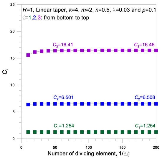
Figure 2. Convergence analysis.

In the available literature, the closed-form or numerical solutions to this problem are lacking, so that, for verification purpose, the selected results of this study are comparable to those of the general-purpose software ADINA and those in the authors’ previous work [17]. The predicted natural frequencies $f_i\left(={\omega }_i/2\pi \right)$ for $k=4$ and $k=\infty$ with the linear taper are compared in Table 2. Here, AFGM is composited with pure aluminum (Al) at the clamped end and pure zirconia (ZrO₂) at the free end, from which the Young’s modulus $E$ and mass density $\rho$ can be defined along with $x$ using Equations (16) and (18). The column parameters are: $R=0,$ $l=1$ m, $V=0.0177$ m³, $n=0.5; E_c=70$ GPa, ${\rho }_c=2700$ kg/m³ (Al); $E_f=140$ GPa, ${\rho }_f=5400$ kg/m³ (ZrO₂); and $P=0$. From these parameters, natural frequencies $f_i=107.8C_i$ Hz are obtained from $C_i$ predicted in this study. Results of this study, ADINA, and reference [17] in Table 2 are in good agreement within a 3.5% error. In these comparisons, the theory, including the numerical method developed herein, is verified.

Table 2. Comparison of frequencies * $f_i$ of this study with those obtained by ADINA and references.

$\mathbf{Side} \mathbf{Number} \mathit{k}$	Data Source	$\mathbf{Natural} \mathbf{Frequency} {\mathit{f}}_{\mathit{i}} \mathbf{in} \mathbf{Hz}$
		$\mathit{i}=1$	$\mathit{i}=2$	$\mathit{i}=3$
4 (Square)	ADINA	155.2	734.4	1867
	This study	156.3	746.6	1925
$\infty$ (Circular)	ADINA	151.8	715.6	1820
	Reference [17]	155.4	742.4	1913
	This study	152.7	729.6	1880

* See the text for column parameters used in the comparison.

Hereafter, the lowest three frequency parameters ($i=1,2,3$) $C_i$ are computed for the numerical experiments. Also $C_i$ with $p=0$ are computed in Table 3, Table 4 and Table 5 since this load case is the most practiced in practical engineering. First, selected analyses were conducted to determine the effects of rotatory inertia index $R$, side number $k$, and taper type on $C_i$, and these results are listed in Table 3, Table 4 and Table 5. Note that the column parameters used in the parametric study are given in each table.

Table 3. Effect of rotatory inertia index $R$ on frequency parameter $C_i$ by volume ratio $\lambda$.

$\mathbf{Volume} \mathbf{Ratio} \mathit{\lambda }$	R	$\mathbf{Frequency} \mathbf{Parameter} {\mathit{C}}_{\mathit{i}}$
		$\mathit{i}=1$	$\mathit{i}=2$	$\mathit{i}=3$
0.005	0	1.449	6.925	17.85
	1	1.449	6.895	17.64
0.01	0	1.449	6.925	17.85
	1	1.448	6.866	17.43
0.03	0	1.449	6.925	17.85
	1	1.445	6.751	16.67
0.05	0	1.449	6.925	17.85
	1	1.441	6.642	16.00

* Linear taper, $k=4$, $m=2$, $n=0.5$, and $p=0$.

Table 4. Effect of side number $k$ on frequency parameter $C_i$.

$\mathbf{Side} \mathbf{Number} \mathit{k}$	$\mathbf{Frequency} \mathbf{Parameter} {\mathit{C}}_{\mathit{i}}$
	$\mathit{i}=1$	$\mathit{i}=2$	$\mathit{i}=3$
3 (Triangle)	1.552	7.227	17.74
4 (Square)	1.445	6.751	16.67
5 (Pentagon)	1.424	6.658	16.46
6 (Hexagon)	1.417	6.629	16.40
7 (Heptagon)	1.415	6.617	16.37
8 (Octagon)	1.413	6.612	16.36
$\infty$ (Circular)	1.412	6.605	16.34

* Linear taper, $m=2$, $n=0.5$, $\lambda =0.03$ and $p=0$.

Table 5. Effect of taper type on frequency parameter $C_i.$

Taper Type	$\mathbf{Frequency} \mathbf{Parameter} {\mathit{C}}_{\mathit{i}}$
	$\mathit{i}=1$	$\mathit{i}=2$	$\mathit{i}=3$
Linear	1.445	6.751	16.67
Parabolic	1.369	6.879	16.93
Sinusoidal	1.414	6.832	16.75

* $k=4$, $m=2$, $n=0.5$, $\lambda =0.03$ and $p=0$.

Table 3 shows the effect of the inertia index $R$ on $C_i$, where the volume ratio $\lambda$ varies from $\lambda =0.005$ to 0.05. From these results, the following findings are observed: (1) $C_i$ is always lower with rotatory inertia $\left(R=1\right)$ than without rotatory inertia $\left(R=0\right)$, as expected based on the free vibration analysis of structures made of conventional homogeneous materials [21]; (2) this frequency reduction is magnified by a higher mode number $i$ and larger parameter $\lambda$; and (3) in practical column designs, the rotatory inertia couple reduces the frequency less than 0.6% for $i=1$, less than 4.3% for $i=2$ and less than 11.6% for $i=3$, which cannot be negligible.

Table 4 shows the effects of side number $k$ on the frequency parameter $C_i$, where the number $k$ varies from $k=3~8$ and $\infty$. Hereafter, all numerical results included the rotatory inertia couple ($R=1$). The frequency parameter $C_i$ with a smaller side number $k$ is larger than $C_i$ with larger $k$. For an illustrative example, the fundamental frequency parameter $C_1$ of $k=3$ (triangle) is 9.9% (1.552/1.412=1.099) larger than $C_1$ of $k=\infty$ even though the column volumes $V$ are the same. When the $k$ value increases, $C_i$ converges to $C_i$ of $k=\infty$. It is observed that $C_i$ for $k=8$ (octagon) approaches $C_i$ for $k=\infty$ within 1.22%. From these results and others not shown, the effect of $k$ is greatly reduced from $i=1$ (critical mode) for the higher mode.

The effects of taper type on the frequency parameter $C_i$, are shown in Table 5. The fundamental frequency parameter $C_1$ is larger in the order from the linear to sinusoidal to parabolic taper, while for the higher modes $i=2$ and $3$, $C_i$ are larger in the order from the parabolic to sinusoidal to linear taper. As an illustrative example, $C_1$ of the linear taper is 5.6% (1.445/1.369 = 1.056) larger than $C_1$ of the parabolic taper and 2.2% (1.445/1.414 = 1.022) larger than $C_1$ of the sinusoidal taper. In higher modes, the effect of taper type may be negligible.

The numerical results for the modular ratio $m$, taper ratio $n$, volume ratio $\lambda$, and load parameter $p$ are presented in Figure 3, Figure 4, Figure 5, Figure 6, Figure 7 and Figure 8, where the effect of rotatory inertia $\left(R=1\right)$ is included. Note that column parameters used in the parametric study are presented in each figure.

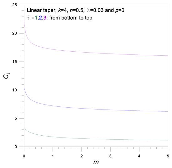
Figure 3. Frequency parameter $C_i$ versus modular ratio $m$ curves.

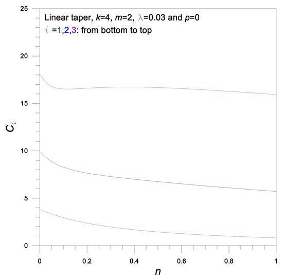
Figure 4. Frequency parameter $C_i$ versus taper ratio $n$ curves.

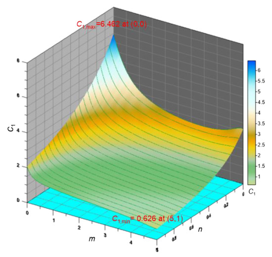
Figure 5. Surface map of $\left(m,n,C_1\right)$ for linear taper, $k=4$, $\lambda =0.03$, and $p=0$.

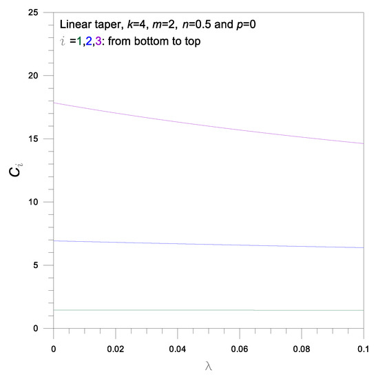
Figure 6. Frequency parameter $C_i$ versus volume ratio $\lambda$ curves.

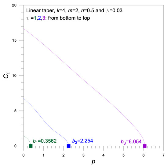
Figure 7. Frequency parameter $C_i$ versus load parameter $p$ curves.

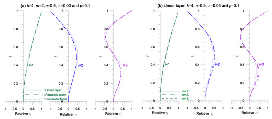
Figure 8. Examples of mode shape (${\xi }_i$,${\eta }_i):$ (a) by taper type; (b) by modular ratio $m.$

Figure 3 presents the frequency curves of $C_i$ versus $m$. The frequency parameters $C_i$ decrease as the modular ratio $m$ increases for all mode numbers $i$. The largest $C_i$ occurs at $m=0$. Higher decreasing rates of $C_i$ are observed for the smaller values of $m$, particularly for $m<1$. Larger values of $m$ lead to smaller reduction rates of $C_i$.

Figure 4 presents the frequency curves of $C_i$ versus $n$. The frequency parameters $C_i$ decrease as the modular ratio $m$ increases for all mode numbers $i$. The characteristics of the frequency curves are similar to those of Figure 3. The largest $C_i$ occurs at $n=0$ and the value of $C_i$ converges to a common value, i.e., $C_i=0$.

Figure 5 represents the three dimensional curved surface map of $\left(m,n,C_1\right)$ with respect to the fundamental frequency parameter $C_1$ in the domain of $0\le m\le 5$ and $0\le n\le 1$ for a given set of column parameters of the linear taper, $k=4$, $\lambda =0.03$ and $p=0$, which is the same as previous Figure 3 and Figure 4. Figure 5 reflects the characteristics of both Figure 3 and Figure 4. The $C_1$ value decreases as both $m$ and $n$ values increase, and therefore the maximum value of $C_{1,\max }=6.462$ occurs at the coordinates $(m=0$,$n=0$) and the smallest value of $C_{1,\min }=0.626$ at the coordinates ($m=5$, $n=1)$, as shown in this figure. If the values $m$ and $n$ are infinitely extended, i.e., zero flexural rigidity $R_f=0$ at the clamped end ($x=0$), the $C_1$ value converges the minimum value of $C_{1,\min }=0$. This means that the cantilever column with the above given set of column parameters has the fundamental frequency parameters $C_1$ in the range of $6.462\le C_1\le 0$.

Figure 6 presents the frequency curves of $C_i$ versus $\lambda$. The frequency parameters $C_i$ decrease as the volume ratio $\lambda$ increases. For the lower modes $i=1$ and 2, the effect of $\lambda$ on $C_i$ is negligible, while for the higher mode $i=3$ not negligible. It is particularly noteworthy that, only in this figure, the angular frequency ${\omega }_i$ with the smaller $C_i$ is larger than ${\omega }_i$ with larger $C_i$, since ${\omega }_i$ is proportional to $\sqrt{\lambda }\left(=\sqrt{l^3/V}\right)$, i.e., ${\omega }_i=(\sqrt{\lambda }\sqrt{E_c/{\rho }_c}/l)C_i$ (see Equation (33)).

Figure 7 shows the frequency curves of $C_i$ versus $p$. The frequency parameters $C_i$ decrease as the load parameter $p$ increases. When $C_i$ decreases and reaches zero, the column buckles and then becomes static state, i.e., $C_i=0$. The corresponding $p$ with $C_i=0$ is the buckling load parameter $b_i$. For an example for the fundamental mode $i=1$, the critical ($i=1$) buckling load parameter $b_{cr}$ is $b_{cr}(=b_1)=0.3562$ is marked by ■ in the horizontal $p$ axis, i.e., $C_1=0$. Using this physical phenomenon, the buckling loads $B$ with natural frequencies of zero can be determined [17]. It is particularly noteworthy that after buckling ($p>b_{cr})$, $C_i$ values are meaningless in practical engineering, since the column has already buckled.

Now, consider the effects of column parameters on the vibration mode shapes. Figure 8 shows examples of the mode shapes for the given set of column parameters presented in this figure. In Figure 8a, three lowest ($i=1,2,3$) mode shapes for the linear, parabolic, and sinusoidal tapers are shown. In Figure 8b, those for $m=1, 2, 3$ are shown. Three mode shapes depicted by solid, dashed, and dotted curves, respectively, in Figure 8a,b, are much different from each other and therefore, the effects of the taper type and modular ratio $n$ on the mode shapes are significant. From these mode shapes, the positions of nodes and maximum amplitudes of the free vibrations are understood.

5. Concluding Remarks

This paper presents a unique numerical approach for analyzing the free vibration of AFG cantilever columns subjected to an axial compressive force. The column is tapered, the cross-sectional shape is a regular polygon, and the volume of the column is constant. A mathematical model of governing differential equations for such columns is formulated based on the dynamic equilibrium of the free body diagram of the column element subjected to the rotatory inertia couple as well as the transverse inertia force. For numerical experiments, the linear functions of Young’s modulus and mass density are selected and three kinds of taper functions of the column are chosen: the linear, parabolic, and sinusoidal taper. The governing equation is numerically integrated by the direct integral method for computing the mode shape, and the determinant search method enhanced by the Regula-Falsi method is used to compute the natural frequencies. For verification purposes, the predicted natural frequencies are compared with those obtained by the general-purpose software ADINA and reference [17]. Effects of the taper type, side number, modular ratio, taper ratio, and volume ratio on the natural frequencies and mode shapes are discussed. For further study, free vibration analysis of AFG columns supported by various end conditions combined with hinged and clamped ends, not considered in this study, is required.

References

- Lee, J.K.; Lee, B.K. Large deflections and buckling loads of cantilever columns with constant volume. Int. J. Struct. Stab. Dyn. 2017, 17, 1750091. [Google Scholar] [CrossRef]
- Horibe, T.; Mori, K. Large deflections of tapered cantilever beams made of axially functionally graded materials. Mech. Eng. Bull. Jpn. Soc. Mech. Eng. 2018, 5, 1–10. [Google Scholar] [CrossRef]
- Akgoz, B.; Civalek, O. Free vibration analysis of axially functionally graded Bernoulli-Euler microbeams based on the modified couple stress theory. Compos. Struct. 2013, 98, 314–322. [Google Scholar] [CrossRef]
- Calio, I.; Elishakoff, I. Closed-form solutions for axially graded beam-columns. J. Sound Vib. 2005, 280, 1083–1094. [Google Scholar] [CrossRef]
- Li, X.F. A unified approach for analyzing static and dynamic behaviors of functionally graded Timoshenko and Bernoulli-Euler beam. J. Sound Vib. 2008, 318, 1210–1229. [Google Scholar] [CrossRef]
- Singh, K.V.; Li, G. Buckling of functionally graded and elastically restrained non-uniform columns. Compos. Part B 2009, 40, 393–403. [Google Scholar] [CrossRef]
- Huang, Y.; Li, X.F. A new approach for free vibration of axially functionally graded beams with non-uniform cross-section. J. Sound Vib. 2010, 329, 2291–2303. [Google Scholar] [CrossRef]
- Shahba, A.; Attarnejad, R.; Marvi, M.T.; Hajilar, S. Free vibration and stability analysis of axially functionally graded tapered Timoshenko beams with classical and non-classical boundary conditions. Compos. Part B 2011, 42, 801–808. [Google Scholar] [CrossRef]
- Shahba, A.; Rajasekaran, S. Free vibration and stability of tapered Euler-Bernoulli beams made of axially functionally graded materials. Appl. Math. Model. 2012, 36, 3094–3111. [Google Scholar] [CrossRef]
- Kukla, S.; Rychlewska, J. Free vibration analysis of functionally graded beam. J. Appl. Math. Comp. Mech. 2013, 12, 39–44. [Google Scholar] [CrossRef]
- Yilmaz, Y.; Zekeriya, G.; Evran, S. Buckling analyses of axially functionally graded non-uniform columns with elastic restraint using a Localized Differential Quadrature Method. Math. Probl. Eng. 2013, 2013, 793602. [Google Scholar] [CrossRef]
- Chandran, G.; Rajendran, M.G. Study on buckling of column made of functionally graded material. Int. J. Mech. Prod. Eng. 2014, 2, 52–54. [Google Scholar]
- Shafiei, N.; Kazemi, M.; Ghadiri, M. Non-linear vibration of axially functionally graded tapered microbeams. Int. J. Eng. Sci. 2016, 102, 12–26. [Google Scholar] [CrossRef]
- Ranganathan, S.; Abed, F.; Aldadah, M.G. Buckling of slender columns with functionally graded microstructures. Mech. Adv. Mater. Struct. 2016, 23, 1360–1367. [Google Scholar] [CrossRef]
- Elishakoff, I.; Eisenberger, M.; Delmas, A. Buckling and vibration of functionally graded material columns sharing Duncan’s mode shape, and new cases. Structures 2016, 5, 170–174. [Google Scholar] [CrossRef]
- Rezaiee-Pajand, M.; Masoodi, A.R. Exact natural frequencies and buckling loads of functionally graded material tapered beam-columns considering semi-rigid connections. J. Vib. Control 2018, 24, 1787–1808. [Google Scholar] [CrossRef]
- Lee, J.K.; Lee, B.K. Free vibration and buckling of tapered columns made of axially functionally graded materials. Appl. Math. Model. 2019, 75, 73–87. [Google Scholar] [CrossRef]
- Gere, J.M. Mechanics of Materials; Brooks/Cole—Thomson Learning: Boston, CA, USA, 2004. [Google Scholar]
- Chopra, A.K. Dynamics of Structures; Prentice Hall Inc.: Upper Saddle River, NJ, USA, 2001. [Google Scholar]
- Burden, R.L.; Faires, D.J.; Burden, A.M. Numerical Analysis; Cengage Learning: Boston, MA, USA, 2016. [Google Scholar]
- Lee, J.K.; Lee, B.K. In-plane free vibration of uniform circular arches made of axially functionally graded materials. Int. J. Struct. Stab. Dyn. 2019, 19, 1950084. [Google Scholar] [CrossRef]
© 2020 by the authors. Licensee MDPI, Basel, Switzerland. This article is an open access article distributed under the terms and conditions of the Creative Commons Attribution (CC BY) license (http://creativecommons.org/licenses/by/4.0/).