Abstract
The study of the combination of chemical kinetics with transport phenomena is the main step for reactor design. It is possible to deviate from the model behaviour, the cause of which may be fluid channelling, fluid recirculation, or creation of stagnant regions in the vessel, by using a dispersion model. In this paper, the known general solution of the dispersion model for closed vessels is given in a new, straightforward form. In order to improve the classical theoretical solution, a hybrid of analytical and numerical methods is used. It is based on the general analytic solution and the least-squares method by fitting the results of a tracer test carried out on the vessel with the values of the analytic solution. Thus, the accuracy of the estimation for the vessel dispersion number is increased. The presented method can be used to similar problems modelled by a partial differential equation and some boundary conditions which are not sufficient to ensure the uniqueness of the solution.
1. Introduction
The efficiency of ensuring stable and economically optimal operating regimes for a wastewater treatment plant requires a mathematical model that describes, using specific tools, the simulation of the technological processes that occur in its operation. As the main technological object of a treatment plant is represented by the biological reactor, the modelling of the complex phenomena that happen in the wastewater flow process, with the help of mathematical models, is a real aid in understanding its functioning, as well as in optimizing the design and the energy consumption.
The study of the combination of chemical kinetics with transport phenomena is the main step for reactor design. Inside of a reactor, the flow pattern usually deviates from the ideal cases of plug flow or mixed flow. This deviation, the cause of which may be fluid channelling, recirculation of fluid, or the fact that stagnant regions were created in the vessel, can be approached by using a model characterized by one parameter (e.g., tanks-in-series model or dispersion model) or a model characterized by two parameters (e.g., reactor with bypassing and dead volume). The parameter(s) of the model is (are) evaluated using the residence time distribution (RTD). MacMullin and Weber were the first who came up with the idea of using the RTD [1]. In the 1950s, Danckwerts proposed the concept of RTD [2], which has been used by many authors. It is mostly associated with the analysis of the chemical reactor performance [3,4,5,6]. A careful analysis of the RTD theory has been published by Nauman [7], who introduced new modelling techniques and applications. The concept of RTD has some limitations mainly for complex systems. In the process simulation of single flow pattern in wastewater treatment, the main restriction is that the process is running under steady-state conditions during the tracer experiment [8]. Therefore, some attempts to use this approach in the transient state were made [9,10,11]. For more than 70 years, this method has been used for process optimization [12,13,14,15,16,17,18].
When we introduce a model pulse of tracer into the fluid that enters a vessel, the pulse spreads while passing through the vessel. If we want to characterize the spreading based on this model, a diffusion-like process superimposed on plug flow, called dispersion or longitudinal dispersion, is assumed [4]. This spreading process is represented by the dispersion coefficient D (). A high value of D denotes the tracer curve rapid spreading, a low value of D represents slow spreading, and D = 0 implies that there is no spreading, hence plug flow. Moreover, the vessel dispersion number, which is a form of the inverse of the Peclet number Pe−1, D/µL where u is the mean (displacement) velocity and L is the length of the vessel, is the dimensionless group characterizing the spread in the whole vessel. If back mixing is transferred on a plug flow of a fluid to a certain degree, whose magnitude does not depend on the position within the vessel, it is called the dispersion model [4]. To solve the problem of dispersion, minimization is a challenging task. There is an extensive literature on the dispersion model [19,20,21,22]. In fact, the dispersion model is based on the dispersion Equation (1) and two boundary conditions, Equations (2) and (3). This problem has infinitely many solutions, but by using additional ideal theoretical conditions, Murphy and Timpany [23] selected an analytic solution described by the residence time distribution (see Equation (33)). However, in the real cases, some errors may often appear by comparing the analytic solution, Equation (33), with the results obtained by measurements (e.g., by so-called tracer test).
In the paper, we introduce a new method for estimating the vessel dispersion number. The outline of this paper is as follows: In Section 2.1, the general solution of the dispersion model for closed vessels is obtained by separation of variables to underline the possibility to improve the known solution obtained by Murphy and Timpany in Reference [23]. Here, a simplified expression of the general solution and of the residence time distribution E(t) is also obtained. Section 2.2 deals with a new solution which is achieved by fitting the results of a tracer test carried out on the vessel with the values of the analytic solution. In Section 2.3, an iterative method to improve the accuracy of the estimation of the parameter D/µL is presented. In fact, an inverse problem is solved by using the results of a tracer test and the least-squares method. An illustrative numerical example is given, and the conclusions of the work are presented in Section 3. The standard tools used for partial differential equations can be found, for example, in Reference [24].
Finally, the given approach is an excellent example of interdisciplinary mathematics with a direct impact on the needs of current industrial practice.
2. Dispersion Model and Its Solutions
2.1. Solution of the Dispersion Model for Closed Vessels
The basic differential equation representing the dispersion model is (see Reference [23,25] or Reference [4]),
where is the concentration (wt./unit vol.) at time t and distance x. We have to take two cases into consideration: boundary conditions for closed vessels and open vessels called Danckwerts boundary conditions (see Reference [3], p. 883). In closed vessels, no dispersion or radial variation in concentration is assumed upstream (closed) nor downstream (closed) of the section where the reaction occurs; therefore, this is a closed-closed vessel. In open vessels, dispersion occurs both upstream (open) and downstream (open) of the reaction section; therefore, this is an open-open vessel. In this paper, we discuss the first case that models all the reactors for which there is no flow or diffusion or up-flow eddies at the entrance or at the vessel exit (see Reference [4]).
Thus, in the case of a closed vessel, plug flow (no dispersion) can be found to the immediate left of the entrance and the immediate right of the exit, so that the boundary conditions can be written in the following form (see Reference [25] or Reference [3], p. 884):
In order to find a solution of Equation (1) that verifies the boundary conditions, Equations (2) and (3) (i.e., to solve the boundary value problem (1)–(3)), the method of separation of variables is used. Thus, by choosing
from Equation (1) it follows that
where is a constant. Hence, the following differential equations are obtained:
and
The general solution of the differential Equation (6) is
where is a constant. Since by (8), it follows that .
By the Equation (4) and using the boundary conditions, Equations (2) and (3), it follows that
and
It is easy to prove that the conditions of Equations (9) and (10) can be fulfilled only in the case when . If we denote by , where is a positive number, then the general solution of the differential Equation (7) is:
where and are constants. Hence, the derivative , is written:
Consequently, from (9)–(12), the following system is obtained:
From the last equation of the system, Equation (13), it follows that
and, by replacing in the first one, we get:
Thus, in order to obtain nonzero solutions of the system, Equation (13), the following condition must be verified:
This condition may be written in the following form:
By denoting
Equation (17) becomes
This can be written in a simplified form if we denote by ,
As can be noticed in Figure 1, Equation (20) has an infinity of solutions which are the abscissas of the intersection points between the graphs of the functions and where . As a matter of fact, there is exactly one solution on each interval ,
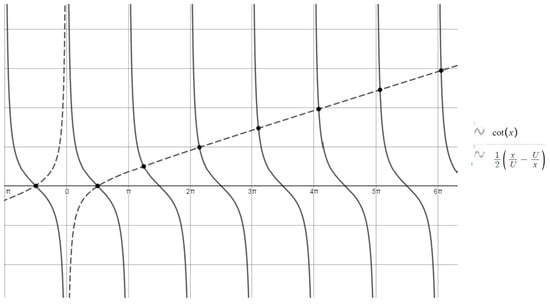
Figure 1.
The solutions of Equation (20).
Now, by Equations (14) and (18), it follows that
and, by Equation (9), we obtain
or, equivalently,
From Equations (4), (8) and (23), the following solutions of the boundary problem, Equations (1)–(3), are obtained:
where , with , are constants. By denoting
Equation (24) becomes
Hence, every finite sum or a suitable infinite series whose terms have the form, Equation (26), is a solution of the boundary value problem, Equations (1)–(3). Thus, the general solution is
where m is either a positive integer or In the second case, also discussed in Reference [23], the constants are small enough such that the series and its partial derivatives converge uniformly on
Let be the mean residence time, which can be written (for a closed system) as . Since
Equation (27) can be written in the equivalent form:
By choosing , where
It follows Equation (10) from Reference [23] expressing the (normalized) residence time distribution :
By taking into account that, for , is the unique solution of Equation (20) on the interval , we obtain that
It follows that
Hence, we obtain a new, simplified expression for the general solution and for the (normalized) residence time distribution . Equations (29) and (33) can be written in the following form:
and, respectively,
2.2. An Improved Solution for the Boundary Value Problem (1)–(3)
In this subsection, we aim to find a solution of the boundary value problem, Equations (1)–(3), more accurate than Equation (36). Consider a sequence of r pairs of real values for :
where is the function defined by Equation (36), are adjustable parameters, and m is a suitable positive integer. The values of will be obtained by fitting the pairs (38) with . Thus, a new solution will be found by considering
As usual in the least-squares method [26], the quantity
must be minimized. Therefore, by using Equation (39), the partial derivatives of the function
with respect to , vanish. Since
the following system of equations is obtained:
where . By solving the system, Equation (43), the constants are obtained and then, by replacing in Equation (39), the solution is determined.
2.3. A New Iterative Method for Estimating the Vessel Dispersion Number
In the case of a closed vessel, the following equation holds as in Reference [3,9,27], or Reference [4], p. 300:
where is the variance. Hence, it follows an estimation of the parameter . In this section we present a new iterative method to increase the accuracy of this estimation. An initial value , determined by Equation (44) using the sequence in Equation (38), is considered. Let m be a fixed positive number less than r. Then, by the system in Equation (43), the values are obtained, and by replacing in Equation (39), the solution is obtained. The main idea is to find a value of such that the corresponding solution provides the minimum value for the function
Since the expression of this function obtained by Equations (39) and (43) is complicated enough to find by analytic methods, a suitable positive small real number is considered. Then, is chosen to be that number from the set
for which the function has the minimum value. If , then can be approximated by . In the case when , the following sequences of values is considered:
Then, is approximated by the first term , for which
Similarly, if , then is approximated by the first term such that
3. Results and Discussion
A first-order reaction takes place in a tubular reactor 6.36 m in length with a diameter of 10 cm (see Reference [3], (p. 889)). The value of the specific reaction rate is 0.25 min−1. Table 1 shows the results of a tracer test performed on this reactor.

Table 1.
The results of a tracer test carried out on this reactor.
By considering a dispersion model of a closed vessel, a comparison between the known analytic method and the new iterative method is given.
In this case and by Equation (44) it follows that , and . Since (see Reference [4], p. 294), we obtain for the values listed in Table 2.
Table 2.
The values of , i = 1,2,…,13.
Then, for , by Equations (20), (30) and (43), we obtain for , and , the values given in Table 3.
Table 3.
The values for , , and , .
The coefficients , i = 1, …, 4 from Table 3 are used in Equation (39) to obtain the solution . The constant C is calculated by using in Equation (32). The value obtained is . New coefficients are calculated afterwards, by the formula . By replacing them in Equation (33), the function is obtained. By comparing (using Equation (45)) the errors obtained for each solution we get that and . Hence, the new solution leads to a better accuracy than In order to improve the accuracy of the new theoretical model, the initial value is considered. By choosing , and , , and using the method from Section 2.2, the corresponding solutions and are determined. Then, and are obtained. Hence, we consider …. and calculate the values of the error function for each case. These values are given in Table 4.
Table 4.
The values of the error function.
The minimum error is obtained for In this case and the graphs of and are represented in Figure 2.
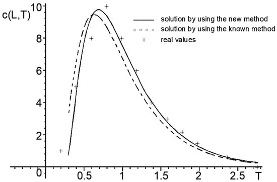
Figure 2.
Real (punctual) values and two approximations of the concentration function: and obtained for .
A comparison of the errors between the real values and those obtained by the classical solution and the new solution is presented in Figure 3.
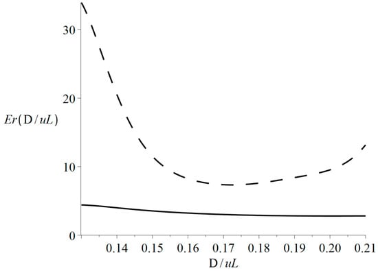
Figure 3.
The errors for the classical solution (dashed line) versus the new solution (solid line).
4. Conclusions
Thus, by this new method, the solution given by Murphy and Timpany [23] can be improved by matching the results of a tracer test performed on the vessel with the values of the analytic solution. Moreover, as a solution of an inverse problem, by an iterative method, the accuracy of the estimation of the vessel dispersion number increased. The presented method can be used to similar problems modelled by a partial differential equation when the known boundary conditions are not sufficient to ensure the uniqueness of the solution.
Author Contributions
Conceptualization, A.-N.D. and G.G.; methodology, M.J.; validation, M.H., and J.V.; formal analysis, L.R.; investigation, A.-N.D. and L.R.; data curation, S.P.; writing—original draft preparation, A.-N.D.; writing—review and editing, G.G., S.P., M.H. and J.V.; visualization, M.J.; supervision, L.R. All authors have read and agreed to the published version of the manuscript.
Funding
This research received no external funding.
Acknowledgments
The second author would like to dedicate this paper to the memory of Eng. Alexandru Braha.
Conflicts of Interest
The authors declare no conflict of interest.
References
- Mac Mullin, R.B. The Theory of Short Circuiting in Continuous-Flow Mixing Vessels in Series and the Kinetics of Chemical Reactions in Such Systems. Trans. Am. Inst. Chem. Eng. 1935, 31, 409–458. [Google Scholar]
- Danckwerts, P.V. Continuous flow systems: Distribution of residence times. Chem. Eng. Sci. 1953, 2, 1–13. [Google Scholar] [CrossRef]
- Fogler, H.S. Elements of Chemical Reaction Engineering, 5th ed.; Prentice Hall: Boston, MA, USA, 2016. [Google Scholar]
- Levenspiel, O. Chemical Reaction Engineering, 3rd ed.; Wiley: New York, NY, USA, 1999. [Google Scholar]
- Nauman, E.B. Chemical Reactor Design, Optimization, and Scaleup, 2nd ed.; Wiley: Hoboken, NJ, USA, 2008. [Google Scholar]
- Froment, G.F.; Bischoff, K.B.; De Wilde, J. Chemical Reactor Analysis and Design, 3rd ed.; Wiley: Hoboken, NJ, USA, 2011. [Google Scholar]
- Nauman, E.B. Residence Time Theory. Ind. Eng. Chem. Res. 2008, 47, 3752–3766. [Google Scholar] [CrossRef]
- Matko, T.; Fawcett, N.; Sharp, A.; Stephenson, T. A numerical model of flow in circular sedimentation tanks. Process Saf. Environ. 1996, 74, 197–204. [Google Scholar] [CrossRef]
- Nauman, E.B. Residence time distribution theory for unsteady stirred tank reactors. Chem. Eng. Sci. 1969, 24, 1461–1470. [Google Scholar] [CrossRef]
- Niemi, A.J.; Zenger, K.; Thereska, J.; Martinez, J.G. Tracer testing of processes under variable flow and volume. Nukleonika 1998, 43, 73–94. [Google Scholar]
- Fernandez-Sempere, J.; Font-Montesinos, R.; Espejo-Alcaraz, O. Residence time distribution for unsteady-state systems. Chem. Eng. Sci. 1995, 50, 223–230. [Google Scholar] [CrossRef]
- Claudel, S.; Leclerc, J.P.; Tétar, L.; Lintz, H.G.; Bernard, A. Recent extensions of the residence time distribution concept: Unsteady state conditions and hydrodynamic model developments. Braz. J. Chem. Eng. 2000, 17, 947–954. [Google Scholar] [CrossRef]
- Bogatykh, I.; Osterland, T. Characterization of Residence Time Distribution in a Plug Flow Reactor. ChemIngTech 2019, 91, 668–672. [Google Scholar] [CrossRef]
- Hohmann, L.; Schmalenberg, M.; Prasanna, M.; Matuschek, M.; Kockmann, N. Suspension flow behavior and particle residence time distribution in helical tube devices. Chem. Eng. J. 2019, 360, 1371–1389. [Google Scholar] [CrossRef]
- Chen, K.; Bachmann, P.; Bück, A.; Jacob, M.; Tsotsas, E. CFD simulation of particle residence time distribution in industrial scale horizontal fluidized bed. J. Powder Technol. 2019, 345, 129–139. [Google Scholar] [CrossRef]
- Deshmukh, S.S.; Sathe, M.J.; Joshi, J.B.; Koganti, S.B. Residence time distribution and flow patterns in the single-phase annular region of annular centrifugal extractor. Ind. Eng. Chem. Res. 2009, 48, 37–46. [Google Scholar] [CrossRef]
- Kolhe, N.S.; Mirage, Y.H.; Patwardhan, A.V.; Rathod, V.K.; Pandey, N.K.; Mudali, U.K.; Natarajan, R. CFD and experimental studies of single phase axial dispersion coefficient in pulsed sieve plate column. Chem. Eng. Res. Des. 2011, 89, 1909–1918. [Google Scholar] [CrossRef]
- Fazli-Abukheyli, R.; Darvishi, P. Combination of axial dispersion and velocity profile in parallel tanks-in-series compartment model for prediction of residence time distribution in a wide range of non-ideal laminar flow regimes. Chem. Eng. Sci. 2019, 195, 531–540. [Google Scholar] [CrossRef]
- Ding, S.; Liu, L.; Xu, J. A study of the determination of dimensionless number and its influence on the performance of a combination wastewater reactor. Procedia Environ. Sci. 2013, 18, 579–584. [Google Scholar] [CrossRef][Green Version]
- Elias, Y.; von Rohr, P.R. Axial dispersion, pressure drop and mass transfer comparison of small-scale structured reaction devices for hydrogenations. Chem. Eng. Process. 2016, 106, 1–12. [Google Scholar] [CrossRef]
- Makinia, J.; Wells, S.A. Evaluation of empirical formulae for estimation of the longitudinal dispersion in activated sludge reactors. Water Res. 2005, 39, 1533–1542. [Google Scholar] [CrossRef]
- Sharma, L.; Nigam, K.D.P.; Roy, S. Axial dispersion in single and multiphase flows in coiled geometries: Radioactive particle tracking experiments. Chem. Eng. Sci. 2017, 157, 116–126. [Google Scholar] [CrossRef]
- Murphy, K.L.; Timpany, P.L. Design and analysis of mixing for an aeration tank. J. Sanit. Eng. Div. 1967, 93, 1–15. [Google Scholar]
- Courant, R.; Hilbert, D. Methods of Mathematical Physics Volume II; Wiley-Interscience: Hoboken, NJ, USA, 1989. [Google Scholar]
- Thomas, H.A.; McKee, J.E. Longitudinal Mixing in Aeration Tank. Sew. Works J. 1944, 16, 42–55. [Google Scholar]
- Borkowski, P. Adaptive system for steering a ship along the desired route. Mathematics 2018, 6, 196. [Google Scholar] [CrossRef]
- Van der Laan, E.T. Notes on diffusion-type model for longitudinal mixing in flow. Chem. Eng. Sci. 1958, 7, 187. [Google Scholar]
© 2020 by the authors. Licensee MDPI, Basel, Switzerland. This article is an open access article distributed under the terms and conditions of the Creative Commons Attribution (CC BY) license (http://creativecommons.org/licenses/by/4.0/).