1. Introduction
Air transport is growing exponentially, from the 3.8 billion air travelers in 2016 to 7.2 billion passengers expected to travel in 2035, according to the International Air Transport Association [
1]. Therefore, air transport and the resulting shortage of laborers in the civil aviation industry has become a serious problem. Air traffic controller (ATC) requires long hours of training, with more than one year needed to train ATCs.
The role of the network manager (NM) is to establish a balance between air traffic demand and airspace/airport capacity in Europe. However, currently, this role is merely moderation between aircraft operators and capacity providers, since the NM has limited instruments to influence either capacity or demand side planning decisions [
2,
3]. The European Commission also recognizes that the lack of the NM’s clear executive powers in practice means that the NM tends to decide by consensus, which often results in weak compromises [
4]. The European Commission however stresses that an optimization of the network performance requires an extended operation scope of actions by the NM, a view also shared by Ryanair [
5].
Although the NM initiates planning several months before the day of operations [
2,
3], most of demand-capacity imbalance situations are still resolved on the day of operations by means of demand management actions, predominantly by delaying flights. For instance, the total en-route air traffic flow management delay was 8.7 million minutes in Europe in 2016, corresponding to a traffic of more than 10 million flights [
3,
6].
More than 55% of total en-route delay is attributed to lack of capacity and staffing reasons, while approximately half of that delay occurred during peak summer months—June, July and August [
3,
6]. The Performance Review Commission notes that the capacity requirements are frequently not met by some area control centres, but also that maximum capacity is not delivered at the times when it is needed [
3,
6].
One of the underlying causes for capacity/demand mismatch is seasonal traffic variability. If traffic is highly variable and there is limited flexibility to adjust the capacity provision according to actual demand, the result may be poor service quality or an under utilization of resources [
6]. If addressed proactively, traffic variability can be mitigated or resolved to a certain degree by utilizing previous experience, roster staffing levels to suit and to make more operations staff available by reducing ancillary tasks performed by ATCs during the peak period [
6]. Meanwhile delay costs occur when there is no sufficient capacity provision for aircraft operators.
In Reference [
7], air traffic control scenarios are classified using decision trees. The authors conclude that decision trees and classification rules perform well in prediction, stability and interpretability.
The activities of the network manager operations center (NMOC) are divided into four phases [
8]—strategic, pre-tactical, tactical and post-operational. The strategic phase is related to capacity predictions at air traffic control centers by air navigation service provides, preparing a routing scheme with the help of NMOC seven days ahead of operations.
The pre-tactical phase is related to the definition of the initial network plan. The NMOC publishes the agreed plan for the day of operations, informing air traffic control units and aircraft operations about the air traffic flow and capacity management measures affecting European airspace from one to six days ahead of operations.
The tactical phase updates the plan for the day of operations according to real-time traffic demand where the NMOC monitors the situation and continuously optimizes capacity. Delays are minimized by providing aircraft affected by changes with alternative solutions on the day of operations.
The post-operational phase is related to operational process improvement by comparing planned and measured outcomes covering all air traffic flow and capacity management domains and units. Operational processes are measured in order to develop best practices and/or analyze lessons learned after the days of operations.
In this paper we focus on the tactical phase, that is, the day of operation. A specific sectorization has been established depending on the aircraft traffic for the considered day and the ATCs have been assigned to the open sectors. We assume that an incident arises, which involves a sectorization change and possibly less available ATCs, and that the available ATCs must be reassigned to the open sectors from that moment until the end of the shift taking into account the work done by each of them from the beginning of the shift to the instant of the incident.
The problem under consideration is similar but different to the shift and break assignment problems, which are referred to in the literature with different names, such as shift design [
9,
10], shift scheduling [
11,
12,
13,
14], break scheduling [
15,
16,
17] and both process shift design and break assignment with a large number of breaks [
16].
Such problems have been extensively investigated in Operations Research and have also recently been tackled with Artificial Intelligence techniques. Also, this is a timetabling and scheduling problem. Timetabling and scheduling problems are combinatorial problems, which, on the grounds of size and complexity, cannot be solved by exact methods within a reasonable computation time. For examples of other timetabling and scheduling problem-solving approaches, see References [
18,
19].
A general mathematical model and specific models for personnel scheduling problems are presented in Reference [
20]. Complexity issues regarding personnel scheduling problems are addressed by identifying polynomial solvable and NP-hard special cases. More recently, a general mathematical model and specific models for personnel scheduling problems were proposed in Reference [
21] enabling the implementation of various heuristic algorithms and their application to a wide range of problems.
Reference [
22] conducted a literature review related to shiftwork management within air traffic management, addressing shiftwork impact on health and safety, productivity and efficiency and discussing issues concerning working time organization in accordance with EC Directive 93/104.
A study on shiftwork practices in both ATM and other fields, such as medicine, the police force and the airline industry, is presented in Reference [
23]. It concludes that, although there are a range of software tools, in many cases involving ATM, they are costly and not completely suited to the needs. The strengths and weaknesses of automated scheduling tools have already been outlined [
24].
Reference [
25] used propositional satisfiability (SAT, [
26]), MaxSAT, the pseudo-Boolean, satisfiability modulo theory, constraint satisfaction and integer linear problem solvers to address a number of different month- or year-long scheduling requirements. According to the results of applying three different optimization techniques jointly with the above problem solvers, SAT approaches appear to come out on top. Then Stojadinovic [
27] combined SAT problem solving with the hill climbing method. The hill climbing method is applied to a feasible solution output by the SAT solver to solve more ATC requirements. The SAT solver is then applied again to further improve the solution. This cycle is iterated until the resulting solution is optimal.
A preliminary approach for modeling many of the features of the ATC scheduling problem was proposed in Reference [
28]. The model divides time into 30-min slots, and an ATC should not work for more than 2 h, followed by at least a 30-min break.
A simplified version of the ATC work shift scheduling problem for Spanish airports was solved by minimizing the number of ATCs required to cover a given airspace sectoring in compliance with Spanish ATC working conditions [
29] in the pre-tactical phase. This problem was mathematically modeled as a mixed integer problem. A simple sectorization for a whole day with 40 available ATCs involved 751,200 variables and more than 161,669 constraints. This makes it hard to reach good solutions in a reasonable time, leading to the use of a metaheuristic.
The search process employs regular expressions to check solution feasibility. Both search processes use regular expressions (regex) [
30]. A regex is a sequence of characters that define a search pattern, used in search algorithms to find strings. The strings represent solutions. The patterns in our approach represent breaches of ATC working conditions.Thanks to the high testing speed and modularity of regex, the optimization model is simpler to implement and maintainable.
A further optimization process is applied to the resulting optimal number of ATCs to balance ATC workloads. There are no constraints on ATC distribution across sectors in this simplified workshift scheduling problem, which accounts for a 24-h period in a core with just one sector.
The proposal reported in Reference [
31] addresses cores with two (en-route and approach) sector types and ATCs with different credentials. Adopting a multi-objective approach, one shift is optimized for a sectorization specified during the pre-tactical phase according to a set number of ATCs considering ATC work and break periods, ATC positions and workload, control center changes and solution structure. The methodology is divided into three optimization phases using a rank-order centroid function to convert a multiple into a single optimization problem taking account ordinal information on objectives (i.e., objectives ranked by importance). First, a template-based method identified unfeasible solutions. Second, independent simulated annealing (SA) output feasible solutions applying regex to check for compliance with ATC working conditions. Third, further independent SA runs optimized the objective functions of these solutions again checking for ATC working condition compliance.
Tello et al. [
32] replaced SA in the third phase of the above methodology with an adaptation of variable neighborhood search. They compared the performance of the two metaheuristics on four different sectorizations supplied by the Spanish ATM Research, Development and Innovation Reference Center (CRIDA). They also compared the run times between regex use and implementation in code to verify ATC working conditions (constraints).
Unlike the problems considered previously [
31,
32], in this paper we focus on the tactical rather than the pre-tactical phase, at the time an incident arises. As said before, a specific sectorization has been established depending on the aircraft traffic for the considered day and the ATCs have been assigned to the open sectors. We assume that an incident happens. Incidents can be of different types: ATCs who cannot continue their working hours because they are unwell or change the sectorization due to a significant increase in air traffic due to diverted air traffic from another airport that has closed for weather reasons.
The incident usually involves a sectorization change. From the moment the incidents occur until the end of the shift the ATCs must be reassigned to the new open sectors taking into account the work done by each of them from the beginning of the shift to the time of the incident and ATC working conditions.
It is important to note that response time is critical in the tactical phase for this variant of the problem. Thus, the use of metaheuristics is even more justified than in the pre-tactical phase.
To solve the problem we propose a methodology that utilizes the metaheuristics simulated annealing and variable neighborhood search, which consists of two phases. In the first phase, it derives a solution, which does not have to be feasible and even need a greater number of ATCs than available ones. This solution in the second phase, applying the metaheuristic, is transformed into a solution in which it need as many ATCs as the number of available ATCs and try to achieve feasibility.
The paper consists of three more sections.
Section 2 shows the proposed methodology for a real time adaptation of the ATC work shift scheduling problem to deal with incidents in airports control centers. The adaptation of SA and VNS to the ATC work shift scheduling problem is explained in
Section 2 Phase 1 and Phase 2, respectively.
Section 3 illustrates the methodology in a real incident from the Barcelona control center. SA and VNS performance has been tested on a set of representative instances in
Section 4. Finally, some conclusions are provided inn
Section 5.
2. Problem Description
Airspace sectorization is the partitioning of the airspace into a given number of sectors. Sectors that are open at any one time should cover total airspace capacity. Additionally, sectors can be clustered together to constitute a core. Nevertheless, a sector may be part of more than one core. An air traffic control center may be in charge of managing one or more cores. Cores are managed separately, although ATCs can be assigned to two or more cores, if sectors they manage belong to more than one core. Sectors are divided into two types depending on their distance from the airport: approach (5 to 10 nautical miles from the airport) and en-route sectors (more than 10 nautical miles from the airport).
Each sector is assigned to a team of air traffic controllers, each of which can handle a limited amount of traffic. Sectors are operated by ATCs with different roles: planner ATCs and executive ATCs. Planner ATCs foresee possible conflicts between aircraft that they report to executive ATCs who instruct pilots on how to avoid loss of minimum separation.
The sector configuration depends on the volume of air traffic. More smaller sectors are opened as the volumen of air traffic grows, increasing the demand for ATCs and vice versa. Therefore, sector configuration and number of ATCs changes as sectors are dynamically divided and merged according to air traffic variations.
Figure 1 shows an example of an airspace sectorization for the Barcelona eastern route. Each time slot has an associated configuration. The number stands for the number of open sectors, and the letter symbolizes the sector configuration. For example, sectorizations 5A and 5B have the same number of sectors with a different spatial distribution.
Besides, in Spain, working conditions are compiled and published in the Official State gazette, Royal Decree 1001/2010, and Law 9/2010. ATC working conditions are as follows:
(LC1) ATCs can only operate sectors belonging to the core for which they are qualified;
(LC2) CON ATCs can only operate en-route sectors;
(LC3) ATCs must rest for 25% of the work shift in day shifts (MS, LMS, AS and LAS). The night shift (NS) break periods account for 33% of working time;
(LC4) A sector opened during the whole night shift must be operated by four ATCs;
(LC5 )ATCs cannot work for more than two hours without a break;
(LC6) ATCs can only operate during one shift;
(LC7) ATCs should rest at least half an hour every two hours;
(LC8) Sector changes are not allowed without resting unless there is an emergency. ATCs can change to an related sector without resting;
(LC9) The minimum work period length of a controller between two breaks is 15 min;
(LC10) Each break period should last at least 15 min;
(LC11) ATCs must remain in the same sector and position for at least 15 min (minimum time in a position);
(LC12) Each ATC can work in at most three different non-related sectors in the respective shift;
(LC13) Each work shift must have one ATC assigned. And each ATC must be responsible of one shift;
(LC14) Each ATC must work at least 15 min, can not rest all the shift.
More details about the problem description are available in Reference [
31].
3. Methodology
The tactical phase takes place on the day of operation, that is, during the work shift. A solution must be found immediately, if an unforeseen event arises, either due to the downgrading of an ATC or the increase in air traffic on any ground. To this end, a two-phase resolution methodology has been proposed.
The starting point for the first phase is the work shifts that were being applied until the unexpected incident occurs. Note that in the considered solutions, time is discretized in slots of five minutes. The slot in which the incident occurs will be called incident slot. This means that the contents of all slots before the incident slot cannot be modified.
We mark the incident slot with a vertical line, see
Figure 2, which shows a solution matrix where each row is an ATC and each matrix element
represents the state of ATC
i in time slot
j. It is symbolized by letters. The value 111 represents a resting ATC, uppercase letters [A–Z] indicate that the ATC is working as an executive operator, whereas lowercase letters [a–z] are used for planner positions.
Depending on the unforeseen event, we will need to modify the sectorization, the solution matrix, and/or the list of available ATCs. For example, the absence of an ATC (by illness or urgency) does not always involve the closure of sectors. Sometimes, the others ATCs can cover the position that has been released until the replacement for a new ATC.
Another example is the closure of an airport because of adverse weather conditions. In that case, traffic will be diverted to nearby airports, which will lead to an increase in air traffic and, therefore, new sectors must be opened. As a result, there would be a change in sectorization and the solution matrix and, possibly, new ATCs must be incorporated to cover new sectors.
The necessary changes will be established by the network manager operations center (NMOC), and constitute an input to the solution algorithm together with the work shifts that are being used.
The aim of the first phase is to modify the work shifts and the list of ATCs in order to incorporate the work slots of the new open sectors in the solution matrix, eliminate the work slots corresponding to the closed sectors, introduce the new ATCs to the ATC list and the shift array, and indicate the downgrading of the ATCs that are not there. Moreover, the largest possible number of available ATCs should remain in the positions (and assigned sectors) that they were working in just after the incident so that not many changes in the control center occur simultaneously. In addition, the only possible solution uses more ATCs that are available in most cases.
The result of the first phase will be used as the initial solution for the second phase. The second phase uses an algorithm based on the metaheuristics simulated annealing or variable neighborhood search to derive a feasible solution that meets all the ATC working conditions (constraints) and reduces the number of shifts to the number of available ATCs.
- Phase 1:
Initialization Algorithm. The initialization algorithm aims at transforming the available solution before the unforeseen event (applied during part of the work shift) into a new solution containing the proposed changes to solve that incident. For this, we divide this phase into the following four steps:
- Step 1:
Closing Sectors. Many times a sector closes and at the same time two sectors related to the closed sector are opened. The objective of this step is to detect closed sectors and their related sectors, in order to replace closed sector working slots with working slots from the new related sectors. The algorithm searches for all closed sectors and checks for related sectors for each of them. In the event that no new opened sectors are found related to the closed sector, the working slots in that sector are replaced by breaks in the solution matrix. Otherwise, that is, there is a new sector to open and this is related to the closed sector, the closed sector working slots are replaced by open and related sector working slots.
- Step 2:
Opening Sectors. When the new sectors are not related to any of the closed sectors, or the closed sectors have already been associated with other related sectors, this step is carried out. The algorithm adds the working slots of the open sectors in work templates (see References [
29,
31,
32]), and adds these templates to the solution matrix. There are several templates that can be used, but we have chosen to apply the template displayed in
Figure 3. The reason for this choice is the ease with which changes can be made to this template without breaking many constraints due to its structure. That template uses three ATCs to cover an entire sector. In this step, more work shifts are added, so there may be more work shifts than ATCs available. However, introducing work slots between ATC breaks would generate shift arrays with a high number of unfulfilled and unstructured constraints or which would make it extremely difficult to the algorithm to work in Phase 2.
- Step 3:
Indisposed ATCs. Another possible incident is the indisposition of an ATC during his/her work shift. In this step, the work shift that the indisposed ATC has associated is modified, and the shift array indicates that this ATC is not available to take on any work from the time the downgrade is set. If his/her work can be assumed and added to the shift of another ATC, it is done, and otherwise, a new work shift will be generated and added to this shift.
- Step 4:
New ATCs. An ATC can be absent, and it is for this reason that there are guard ATCs to solve these kind of situations. The guard ATCs have a deadline to show up at the control center since the notice occurs. Therefore, we can count on new ATCs when it comes to spreading the workload. In this step, we add the new ATCs to the ATC’ list and add a new shift for each new ATC, which supports work from the moment the ATC arrives at the control center. Finally, this shift is associated with the new ATC.
Once the four steps of the initialization algorithm have been performed, we have an initial solution to start with Phase 2. For this, the solution must comply with the following premises:
All sectors must be covered in both work positions (executive and planner) all the time.
All ATCs must have an associated shift in the shift list, although there can be work shifts not assigned to ATCs (assigned to imaginary ATCs).
All ATCs must be listed in the ATC list.
- Phase 2:
Metaheuristic-based optimization process. Phase 2 consists of applying a metaheuristic: simulated annealing (SA) or variable neighborhood search (VNS). The goal of this phase is to reach a feasible solution that meets the modifications made to address the unforeseen event. For this, we simultaneously consider four objectives. First, an initial solution in Phase 1 may use more than the available number of ATCs. Therefore, they need to be reduced until the number of required ATCs matches the number of available ATCs.
Secondly, the solution must be feasible. All ATC’s working conditions must be met and all open sectors in both positions (executive and planner) must be covered all time.
The third objective consists of minimizing the number of changes during the incident slot, that is, try to ensure that ATCs are kept in the same position just after the incident. At that point, several sectors may open or close and some ATCs change their job in a forced way, so we’re going to try to minimize the number of changes to avoid that all ATCs get out of their position simultaneously as much as possible.
The last objective refers to a similar solution structure to previous template-based solution. Control center staff will find such a solution easier to understand, and this should facilitate any manual changes.
The target function in both SA and VNS is a weighted sum of the four objectives that are explained in detail below.
Reduce the number of shifts until the number of available ATCs: It is important to note that in the solutions we are analyzing, shifts are ordered from the least to the highest workload (in the first rows the lowest load and the last ones with the highest load).
However, when sorting shifts, let’s divide the array into two sections: shifts that have an assigned ATC and shifts that do not have assigned an ATC. In this way, shifts without an assigned ATC will occupy the first rows of the array sorted by workload, while shifts with an assigned ATC will be sorted between them subsequently. With this we aim to encourage the shifts that are going to be eliminated are the shifts without assigned ATCs. To do this, we use the following expression:
where,
nATC is the number of shifts and
the number of shift work slots (in the
k-th row of the solution coding).
In Equation (
1), the product of the numerator causes the
p-value to be higher the higher are the shifts of the last rows (that is, those with the highest workload). Therefore, in the search process, the workload of the shifts from the first rows to those of the last rows will tend to be passed, causing the shifts of the first rows to run out of load and be able to be deleted. The denominator of the array is squared so that the solution is always improved by deleting a turn. Otherwise, it could happen that by removing a turn to worsen fitness.
We must normalize Equation (
1) to be used in the objective weight addition as follows:
where
and
are maximum and minimum values of
p, respectively.
To describe the way
and
are computed, we must first introduce a new term,
. To calculate this value, the total workload is computed from the sectorization. This gives us a number of work slots that should be split across all shifts, denoted as
and to get
:
Equation (
3) refers to the number of ATCs needed that have to work the entire shift in order to cover the workload,
. Once this value is known, we can calculate the value of
as follows
where we assign the maximum workload to the shifts that are in the last rows, while the first ones are not assigned by the workload.
is computed from the following expression:
where we don’t assign workload to shifts in the last rows, but shifts in the first rows are assigned the maximum workload.
Reduce the number of unfulfilled constraints: ATCs’ shifts must comply with all working conditions. To make this possible, we have introduced the number of unfulfilled constraints within the target function, denoted by .
We transform the equation into a maximization form and normalize it, leading to the following expression:
where
is the maximum value that can be achieved by breaking all constraints.
For the calculation of we must consider two cases:
Night shift. In this shift all constraints apply so
is calculated as follows: there is a total of 14 constraints. 8 constraints can be breached
times, 2 constraints that can be breached
and 4 constraint can be breached
multiplied every time it is not met in each slot of the shift by
, that is,
. Then, we have:
that is,
.
Day shifts (morning and afternoon). One constraint does not apply, so we’ll use Equation (
8):
that is,
.
As the incident management may lead to unfeasible solutions, weights representing the relative importance of constraint violation were introduced by experts from CRIDA (
www.crida.es), a non-profit joint venture between ENAIRE, Spain’s air navigation manager, the Universidad Politécnica de Madrid, and Ineco, a global infrastructure engineering and consultancy leader.
First, a subset of the most important (priority) labor constraints was identified (LC1-LC7, LC9, LC12-LC14) (weight 5), followed by LC8 (weight 0.9), LC11 (weight 0.85), LC10 (weight 0.96) and LC9 (weight 0.5). Thus, we should attempt to meet the constraints in the most important set in preference to the other constraints.
Reduce the number of changes during the incident slot: To avoid a simultaneous change of a large number of ATCs just after the incident we use the following expression:
where
is the contents of the slot in the shift
i and the incident slot
c, whereas
is the content of the slot in the shift
i and the slot before the incident slot.
Maintain solution-like structure: The aim is to derive a solution as compact as possible. For this, we use the following expression, where each is time slot is compared against the one on his right and under it:
In Equation (
10) is checked for each
, if the slot on its right (
) has the same content and if so, add 1, also checks if the slot below (
) has the same content and if so adds to 0.2. If both are different, no value will be added. To get the theoretical maximum value we use the Equation (
11).
This is a theoretical maximum value without regard to constraints. Once we have this value we can normalize the target with the Equation (
12).
Once all four objectives are calculated, a weighting is made between all objectives to obtain the target function:
CRIDA experts ranked the above objectives by importance, and the weights were derived using a rank-order centroid (ROC) method [
33].
The following sections describe the adaptation of SA and VNS to our ATC work shift scheduling problem and the corresponding parameter tuning are described.
3.1. Simulated Annealing Adaptation
Simulated annealing (SA) [
34,
35] is a trajectory-based metaheuristic which is named for and inspired by annealing in metallurgy. SA is one of the oldest metaheuristics and has been adapted to solve many combinatorial optimization problems. Over the years, many authors have proposed both general and problem-specific improvements and variants of SA [
36]. Different variants of scheduling problems have been tackled using SA [
37], such as the job-shop scheduling problem [
38,
39,
40,
41], university course timetabling problems [
42], or sports scheduling problems [
43].
SA pseudocode for a minimization optimization problem is shown in Algorithm 1. The basic idea of SA is as follows. An initial feasible solution, , is randomly generated. Then, in each iteration i, a new solution (y) is randomly generated from the neighborhood, , of the solution considered in that iteration, . If the new solution is better than the current one, then the algorithm moves to that solution. Otherwise, there is some probability of it moving to a worse solution. The acceptance of worse solutions makes for a broader search for the optimal solution and avoids trapping in local optima in early iterations.
The search is initially very diversified, since practically all moves are allowed. As the temperature drops, the probability of accepting a worse moves decreases, and only better moves will be accepted when it is zero. This makes SA work like hill climbing.
Some elements in the above algorithm require clarification. Numerous studies propose techniques to calculate initial temperature (
) that allow an acceptance rate of about 95% of solutions. However, in this case we prefer to reduce the acceptance rate to 60% due to the nature of the problem to avoid an unnecessary scan that entails a high computation time. This allows us to perform a slower temperature drop without wasting exploration time in unpromising search spaces.
| Algorithm 1 Basic SA. |
| 1: Do , , Select the initial temperature ( temperature in step i) |
| 2: repeat |
| 3: Randomly generate |
| 4: if ( then |
| 5: |
| 6: if ( then |
| 7: |
| 8: end if |
| 9: else |
| 10: |
| 11: if ( then |
| 12: |
| 13: else |
| 14: |
| 15: end if |
| 16: end if |
| 17: Update temperature, |
| 18: until stopping criterion |
Regarding the temperature update, after running different tests looking for the best cooling function, we found that, in this case, the classic geometric function is the most promising function:
The number of iterations in which the temperature is kept constant influences the evolution of the temperature. We use the cutoff method, which is to incorporate a counter of the number of improving iterations and, when it exceeds a threshold (1000 iterations), the temperature may drop before the established.
Besides, choosing solutions from a neighborhood () is one of the most important points for the proper operation of SA, and, for this reason, different neighborhood definitions have been tested. Several movements have been proposed for this problem and, after a comparison process, the following movement was chosen.
Starting with the initial solution, the solution is divided into different sets of slots using a grid. This grid sets the cuts at different points where there are changes from work to rest or from one sector to another.
Figure 4 shows an example of how a grid would be created from an initial solution.
The grid sets the start and end points of the different sets of slots that allow permutations along the iterations of the algorithm, and the movement is defined as the exchange of the set of slots between two distinct rows. We have an example of movement in
Figure 5.
Throughout the execution, in order to promote exploitation, the grid is modified reducing the size of the spaces to a minimum number of slots. This initially achieves greater exploration and increased exploitation as iterations progress.
The acceptance function is a method that allows us to move towards worse solutions than the current one with some probability. There are several functions to determine the likelihood of acceptance
p of these solutions. Equation (
15) shows the chosen function.
where
is the a random solution in the neighborhood of actual solution
and
is the temperature in step
i.
Finally, the stopping condition sets when the algorithm should stop. We use a solution improvement-related condition: the algorithm is stopped when the best solution found is not improved within a certain number of iterations. This threshold has been set at 50,000 iterations.
3.2. Variable Neighborhood Search Adaptation
Variable neighborhood search (VNS) is based on the idea of successively exploring a set of neighborhoods to solve optimization problems [
44]. VNS explores neighborhoods either at random or systematically in search of local optima. Local searches of different neighborhoods should generate different local optima, and the global optimum will be a local optimum for one such neighborhood.
Algorithm 2 illustrates the basic version of VNS. There are many other variants of VNS in the literature, including variable neighborhood descent, reduced variable neighborhood search and variable neighborhood decomposition search. They differ according to:
Neighborhood order: forward VNS starts with and increases k by one if no better solutions are found; otherwise it sets ; backward VNS starts with and decreases k by one if no better solutions are found, and extended VNS uses parameters and , sets and increases k by if no better solution is found.
Solution acceptance: skewed VNS accepts worse solutions if , where is the distance between candidate solutions.
| Algorithm 2 Basic VNS. |
| Require:: set of neighborhood structures, |
| Ensure: Best solution found. |
| 1: |
| 2: Generate an initial solution x |
| 3: repeat |
| 4: Randomly generate |
| 5: = Local-search(,) |
| 6: ifthen |
| 7: |
| 8: |
| 9: else |
| 10: |
| 11: end if |
| 12: until stopping criterion |
We used variable neighborhood descent (VND) [
45]. This deterministic algorithm selects an initial solution and iterates through all the selected neighborhoods in the specified order, running a search process to find a local optimum in each iteration. If this local optimum is found to be better than the incumbent best solution, it becomes the new initial solution for a local search. If not, the algorithm explores the next specified neighborhood.
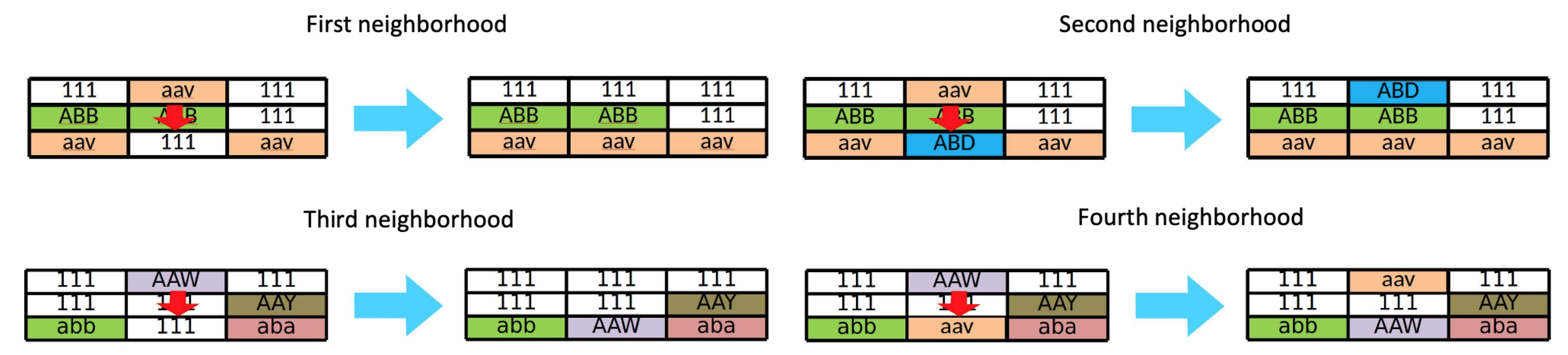
It includes four types of neighborhoods, see
Figure 6.
Neighborhood 1: Time slot exchange between to ATCs subject two the following constraints:
ATCs remain in the same sector and position (planner or executive) for approximately 45 min.
Optimally, ATCs should work for 90 min between breaks.
ATCs should spend from 40% to 60% of working time in executive positions.
Neighborhood 2: Time slot exchange between two ATCs subject to the following constraints
ATCs remain in the same sector and position (planner or executive) for approximately 45 min.
Optimally, ATCs should work for 90 min between breaks.
ATCs should spend from 40 to 60% of working time in executive positions.
Exchanged time slots must be work periods.
Neighborhood 3: Time slot exchange between two ATCs subject to the following constraints:
ATCs remain in the same sector and position (planner or executive) for approximately 45 min.
Optimally, ATCs should work for 90 min between breaks.
ATCs should spend from 40 to 60% of working time in executive positions.
One ATC was working in the same sector and position immediately before or after the exchange time slot (no work period extension is required).
Neighborhood 4: Time slot exchange between two ATCs subject to the following constraints:
ATCs remain in the same sector and position (planner or executive) for approximately 45 min.
Optimally, ATCs should work for 90 min between breaks.
ATCs should spend from 40 to 60% of working time in executive positions.
Exchanged time slots must be work periods.
One ATC was working in the same sector and position immediately before or after the exchange time slot (no work period extension is required).
4. An Illustrative Example
We now illustrate the operation of the problem-solving methodology explain above using a real example of application from the Barcelona control center originated during an afternoon shift, referred to henceforth as Instance 1.
Note that a control center may be responsible for managing one or more cores. Each core should be solved separately, unless there are sectors belonging to more than one core. In this case, ATCs should be assigned to the respective cores. The Barcelona control center manages two cores, the western route and the eastern route cores, and the sectors under consideration in this instance belong to only one of these cores. Thus, each core can be solved separately.
The shift lasts from 15:00 to 21:35, the sectorization established is shown in
Figure 7, a 04A configuration (sectors adc, aee, acy, adu) for the
western route core and a 05A configuration (sectors adq, adl, adp, adr, aea) for the
eastern route core.
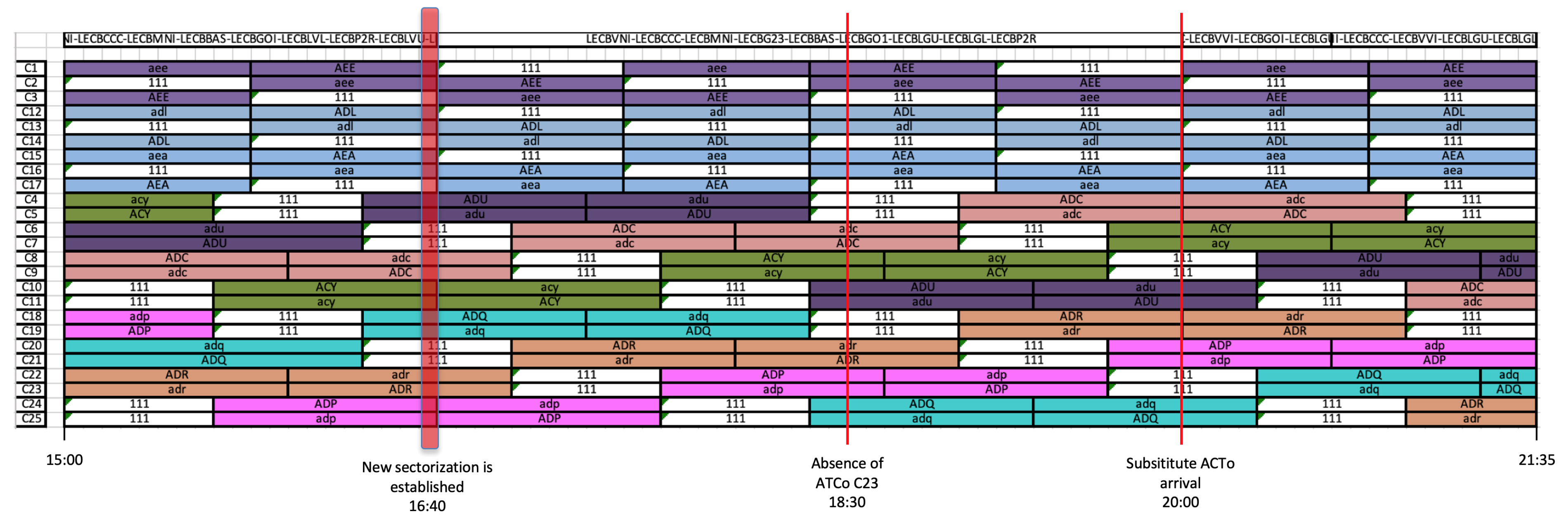
Figure 8 shows the solution (ATCs shifts) covering the sectorization established before the incident. The number of available ATCs is 25, 11 (C1–C11) belonging to the eastern route core and 14 (C12–C25) to the western route core.
The incident in question is as follows. An ATC has to leave his/her workplace, leaving a vacant slot at 18:30, that is, three and a half hours after starting the shift, see
Figure 8. The manager reports the incident and notifies a substitute ATC who should provide support to his/her colleague. However, the substitute cannot get up until one and half hours later (20:00). In addition, one of the open sectors is closed as a result of an expected decline in air traffic. In response to the incident, a new sectorization is established at 16:40, as shown in
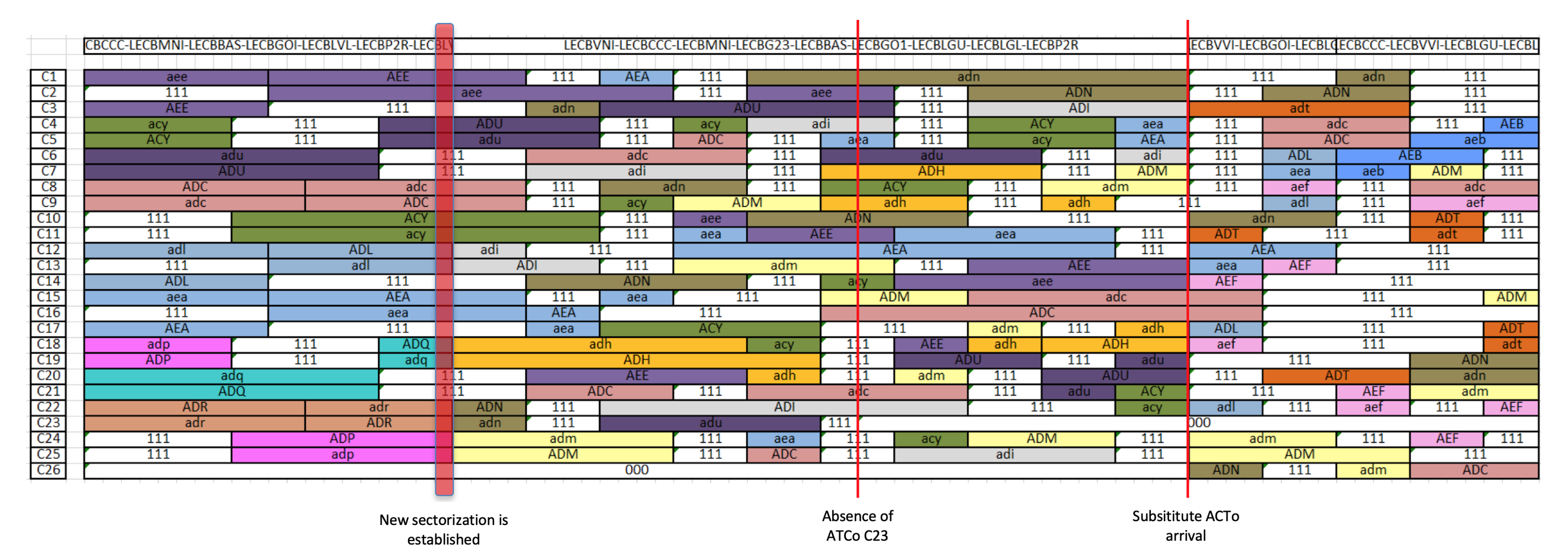
Figure 9.
In the new sectorization, there are six open sectors in the Barcelona western route core: a 04A configuration (sectors adc, aee, acy, adu) from 15:00 to 20:00, and a 03A configuration (sectors adc, adt, aef) from 20:00 to 21:35; and 10 sectors open in the Barcelona eastern route core: a 05A configuration (sectors adl, adp, adr, adq, aea) from 15:00 to 16:40, a 05C configuration (sectors aea, adi, adn, adh, adm) from 16:40 to 20:00, a 04A configuration (sectors adl, aea, adn, adm) from 20:00 to 20:40, and a 03A configuration (sectors adn, adm, aeb) from 20:40 to 21:35 (see
Figure 9).
The first phase of the problem-solving methodology modifies the current ATC working time (shown in
Figure 8) to output a new schedule including all the modifications required to deal with the unforeseen event.
The solution derived from the first phase is shown in
Figure 10. Even though it includes four more than the available ATCs (denoted as C0, see the first four lines in
Figure 10) and is not feasible, this solution accounts for all the necessary changes to meet the new working hour requirements and will be the starting point of the second phase. The solution shows that ATC C23 (ATC absent from his/her position at 18:30) and C26 (substitute ATC getting up at 20:00) are not working the shift, neither will be able to assume workload from 16:30 to 20:00. ATCs not working the shift are represented by the string “000”.
In the second phase, SA and VNS are used to derived a final solution.
In SA, the parameters are set as follows. Initial temperature is , which stands for a low acceptance rate. This is because the time available to solve the problem is limited, and it is inconvenient to break the built-in structures of the solution. The proposed cooling function uses a cooling ratio of , and the temperature is reduced every iterations. Besides, the cutoff method lowers the temperature without having to wait for the specific number of iterations if 1500 iterations consecutively improve the current solution.
Finally, SA and VNS both use the following stopping criteria: both stop the execution if there is no improvement of 0.02% in the target value corresponding to the best solution found for 50,000 iterations.
At the end of the second phase, we have the best solution so far.
Figure 11 and
Figure 12 show the solution reached by SA and VNS, respectively, where the four artificial ATCs (C0) are no longer present as the other ATCs have taken on their workload. In addition,
Table 1 shows the values for the different objective functions and the respective computation times.
Note that a value of means that the solution uses no more than the number of available ATCs, whereas means that all the ATC working conditions are met, and, consequently, the solution is feasible. Thus, the solution reached by SA is feasible, whereas the solution derived by VNS uses the available number of ATCs but violates 26 constraints.
The proportion of ATCs who do not change their position during the incident slot is the same in both solutions (0.6923). Eighteen out of the 26 ATCs are kept in the same position just after the sectorization change (incident slot). The SA solution outperforms the solution derived by VNS with regard to
, that is, the SA solution is more compact, which makes it easier to understand for the NMOC (see
Figure 11 and
Figure 12).
Finally, it takes considerable less time for VNS to reach the solution (1.02 min) than SA (10.45 min). We can conclude that SA outperforms VNS with regard to the solution quality ( and ), but VNS reaches the final solution faster. However, the SA computation time also satisfies CRIDA experts.
Table 2 shows information about the constraint violation distribution using VNS. Priority constraints are highlighted in bold. Four out the fourteen constraint types are not met, and two priority constraints (LC5 and LC12) are not met four and eight times, respectively.
5. Numerical Analysis
Simulated annealing (SA) and variable neighborhood search (VNS) performance has been tested on a set of representative instances provided by CRIDA experts (see
Table 3).
Instance 1 was used to illustrate the proposed methodology in
Section 3. Instance 2 also refers to the Barcelona control center but is centered on a morning shift with a different number of available ATCs and a different incident. Instances 3, 4 and 5 focus on the Madrid control center on an afternoon shift with the same number of available ATCs but different incidents. Finally, instances 6 and 7 address the Gran Canaria control center during a morning shift with 25 available ATCs and one absent ATC absence, in the first case, plus a substitute ATC in the second instance.
In the following sections, we describe Instances 2–9 in detail, show the solution before the incident, plus the solutions derived from Phases 1 and 2 and compare the solutions reached using SA and VNS.
5.1. Instance 2
Instance 2 is a real case of a morning shift turn at Barcelona control center from 7:30 to 15:00. Two cores are managed simultaneously, as in Instance 1. The number of available ATCs is 24, seven belonging to the eastern route core and 17 to the western route core.
In the new sectorization, the western route core does not undergo any change with three open sectors throughout the shift. However, the eastern route core moves from five to six open sectors (sector adl is closed and sectors adg and adk are opened) at 10:30, which remains so for four and a half hours until the end of the shift.
Figure 13 shows the solution before the incident, the solution derived in Phase 1 and the solution derived in Phase 2 using SA for Instance 2.
The first phase modifies the initial working time of ATCs to output a new schedule incorporating all modifications to deal with the unforeseen event. Three more ATCs than are available (denoted as C0, see the first three lines in
Figure 13) are used to cover the new open sector adk. Therefore, the solution is not feasible.
Table 4 shows the values of the different objective functions for the SA and VNS solutions in the seven instances under consideration and their computation times.
As mentioned for Instance 1, a value of means that the solution uses no more than the available number of ATCs, whereas means that all the ATC working conditions are met, and, consequently, the solution is feasible. Thus, the solutions reached by SA and VNS in Instance 2 use the number of available ATCs but violate six and 49 constraints, respectively. All ATCs remain in the same position during the incident slot in both solutions (), and the SA solution outperforms the solution derived using VNS with regard to , that is, the SA solution is more compact. This makes it easier to understand for the NMOC.
Although Instance 2 looks simple, the incident is very complex to manage. The solution before the incident is composed of 24 ATCs covering 9 (3 × (3 × 8)) sectors, and the percentage break time for ATCs is 25%, which exactly matches a labor constraint. Thus, ATCs do not have even one extra minute of break time. Besides, it accounts for two cores simultaneously, and the different ATCs can only be assigned to the sectors belonging to the core in which they are working. This further restricts the problem resulting in very few feasible solutions, as the working margin is very small. Consequently, it should be no surprise if a feasible solution is not reached.
Finally, the time it takes VNS to reach the solution (1.83 min) is considerably less than for SA (13.32 min). The latter is considered very satisfactory by CRIDA experts.
Table 5 shows information about the constraint violation distribution using both SA and VNS in the instances under consideration. Priority constraints are highlighted in bold.
In Instance 2, as mentioned above, the SA and VNS solutions failed to met six and 49 labour constraints, respectively. The six constraints are not met by the SA solution are priority constraints (LC9 three times and LC12 three times). Twenty-five out of the 46 constraints not met by the VNS solution are priority constraints (LC3 and LC5 five times each, LC9 once and LC12 14 times). SA clearly outperforms VNS with respect to this objective.
5.2. Instance 3
Instance 3 refers to a real case of an afternoon shift at Madrid control center from 15:30 to 22:30. Only one core is managed, and the number of available ATCs is 19.
The incident involves the closure of several sectors, moving from a sectorization with seven open sectors throughout the shift to seven sectors open until 20:40. At this time, two sectors are closed and the other five sector are kept open until 21:00, when another sector is closed. Then, the four sector are kept open until 21:40, when another sector is closed until the end of the shift (three open sectors).
Figure 14 shows the solution before the incident, the solution derived in Phase 1, and the solution derived in Phase 2 using SA on Instance 3. Artificial ATCs (C0) do not have to be used in Phase 1.
Looking at
Table 4, we find that the solutions reached by SA and VNS for Instance 3 both use the available number of ATCs, but violate two labor constraints, corresponding to LC11 (twice). LC11 is not a priority constraint (
Table 5).
Note that a feasible solution can never be reached for Instance 3 due to the position of the incident slot. The minimum consecutive working time of ATCs working in the sector that is closed as a consequence of the incident is irreparably violated, and the problem-solving method cannot modify any slot in the solution before the incident slot. The proportion of ATCs who remain in the same position during the incident slot is the same in both solutions (0.4736). Nine out of the 19 ATCs remain in the same position just after the sectorization change (incident slot).
The SA solution outperforms the solution derived by VNS with regard to , that is, the SA solution is more compact, which makes it easier to understand for the NMOC. Finally, the time it takes for VNS to reach the solution (0.13 min) is slightly lower than for SA (6.35 min)—The latter is considered very satisfactory by CRIDA experts.
The solutions derived by SA and VNS for Instance 3 are equal with regard to objectives , and , where the SA solution is better in terms of compactability, and VNS has a lower computation time (SA computation time also satisfies the CRIDA experts).
5.3. Instance 4
Instance 4 refers to a real case of an afternoon shift at Madrid control center from 15:30 to 22:30. Only one core is managed, and the number of available ATCs is 19.
The incident involves the closure of several sectors, like Instance 3. It passes from a sectorization with seven open sectors throughout the shift to seven sectors open until 20:40. At this time, two sectors are closed, and five sectors are kept open until 21:00, when another sector is closed. Then, the four sectors are kept open until 21:40, when another sector is closed until the end of the shift (three open sectors).
Additionally, an ATC (C8) has to leave his/her position, leaving a vacant slot at 17:00, that is, two and a half hours after starting the shift. The manager reports the incident and notifies a substitute ATC who should provide support to his/her colleague, but the substitute cannot get up until three hours and 20 min later (20:20),
Figure 15.
Figure 15 shows the solution before the incident, the solution derived in Phase 1, and the solution derived in Phase 2 using SA on Instance 4.
The first phase modifies the initial working time of ATCs to output a new schedule incorporating all modifications to deal with the unforeseen event. One more than the available ATCs (denoted as C0, see the first line in
Figure 15) is used, and it is, therefore, a feasible solution.
Looking at
Table 4, we find that the solution reached by the SA is feasible, whereas the solution derived by the VNS uses the number of available ATCs but does not met four constraints, violating LC3, LC5, LC8 and LC11 once each, where the first two are priority constraints (
Table 5). The proportion of ATCs who remain in the same position during the incident slot is higher in the VNS solution, where 16 out of the 19 ATCs remain in the same position just after the sectorization change (incident slot). There is an additional change in the SA solution.
The SA and VNS solutions are equal in terms of compactability, . However, VNS is again faster at reaching the solution (0.6 vs. 6.21 min). Given that the SA computation time also satisfies the CRIDA experts, the SA solution involves no more than an additional control center change (in the incident slot) but is a feasible solution (the VNS solution violates four of the labor constraints), the SA solution was selected for Instance 4 by CRIDA experts.
5.4. Instance 5
Instance 5 refers to a real case from the afternoon shift at Madrid control center from 15:30 to 22:30. Only one core is managed, and the number of available ATCs is 19.
The incident in question involves the closure and opening of several sectors. It passes from a sectorization with seven open sectors throughout the shift to seven open sectors until 17:40. At this time, an additional sector is opened, and the eight sectors are kept open until 20:40, when a sector is closed. Then, the seven sectors are kept open until 21:00, when the sectorization changes and only four open sectors are established. A sector is closed 20 min later (21:20), and the three sectors are kept open until the end of the shift.
Figure 16 shows the solution before the incident, the solution derived in Phase 1, and the solution derived in Phase 2 using SA on Instance 5.
In the first phase, three more ATCs than available (denoted as C0, see the first three lines in
Figure 16) are incorporated to manage the newly opened sector, abv.
Looking at
Table 4, we find the solutions reached by SA and VNS for Instance 2 use the available number of ATCs but violate six and nine constraints, respectively. Four out the six labor constraints not met by the SA solution are priority constraints (LC5 four times). C12 is also violated twice (
Table 5). Eight out the nine labor constraints not met by the VNS solution are priority constraints (LC3 once and LC5 seven times).
The incident in Instance 5 involves a high workload. Therefore, it is impossible to find a feasible solution because the difference between the workload (8 sectors × 2 positions × 36 slots (3 h) = 576) and the ATC-assumed work ((19 ATCs × 36 slots − 6 slots (mandatory timeout)) = 570) is slots, without counting the ATC labor constraints. The proportion of ATCs who do not change their position during the incident slot is 0.7894 in both solutions. Fifteen out of the 19 ATCs remain in the same position just after the sectorization change (incident slot).
The SA solution outperforms the solution derived by VNS with regard to , that is, the SA solution is more compact, which makes it easier to understand for the NMOC. However, VNS is again faster at reaching the solution (0.47 vs. 11.18 min). SA outperforms VNS with regard to objectives and , but VNS has a lower computation time. As SA computing time also satisfies the CRIDA experts, the SA solution is chosen for Instance 5.
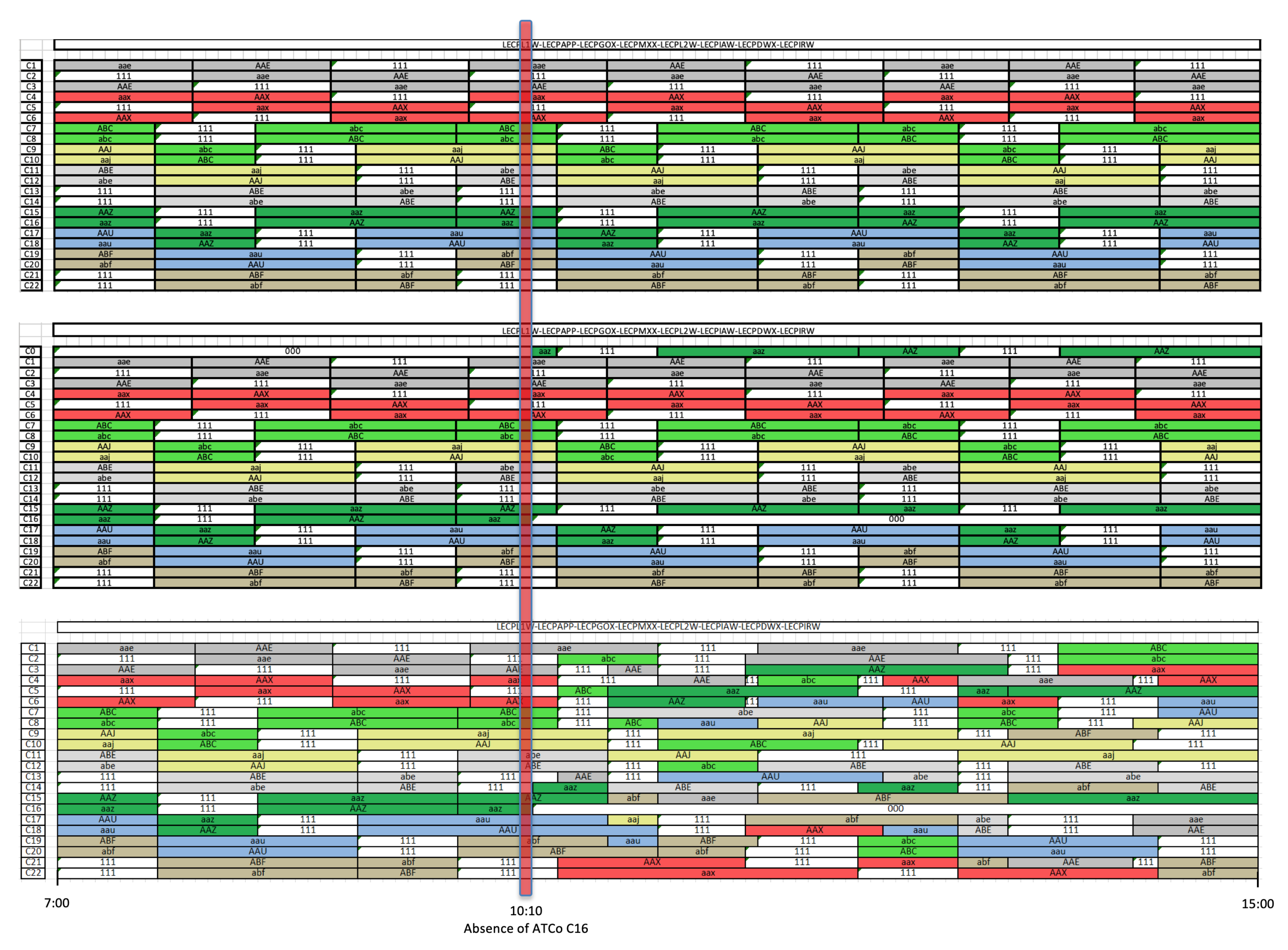
5.5. Instance 6
Instance 6 is a real case from the morning shift at Gran Canaria control center. An 8A sectorization is used throughout the shift, from 7:00 to 15:00. There are 22 available ATCs to cover this sectorization, but ATC C16 is relieved at 10:10, and no substitute is available. Therefore, the remainder of the shift is covered by 21 ATCs.
Figure 17 shows the solution before the incident, the solution derived in Phase 1, and the solution derived in Phase 2 using SA.
In the Phase 1 solution, the workload of ATC 16 is assigned as of 10:10 to ATC C0 (artificial ATC). This workload is distributed among the other ATCs in Phase 2, and the artificial ATC is no longer necessary.
In Instance 6, the solutions reached by SA and VNS for Instance 2 use the number of available ATCs but violate eight and 18 constraints, respectively, see
Table 4. Four out of the eight labor constraints not met by the SA solution are priority constraints (LC3 once, LC5 once and LC10 four times). LC10 is also violated four times (
Table 5). The 18 labor constraints not met by the VNS solution are priority constraints (LC3 five times, LC5 five times and LC12 five times).
The solution for Instance 6 involves a high workload. Therefore, it is impossible to find a feasible solution because the difference between the workload (8 sectors × 2 positions × 96 slots (8 h) = 1536) and the ATC-assumed work ((22 ATCs × 38 slots + 21 ATCs × 58 slots) × 3/4 (25% mandatory timeout) = 1540) is slots. The proportion of ATCs who do not change their position during the incident slot is 0.9047 in both solutions. Nineteen out of the 21 ATCs remain in the same position when ATC 16 is relieved.
The SA solution outperforms the solution derived from VNS with regard to , that is, the SA solution is more compact, which makes it easier to understand for the NMOC. However, VNS is again faster at reaching the solution (0.53 vs. 11.52 min). Given that the SA computation time also satisfies the CRIDA experts, and the SA solution violates fewer labor constraints and is more compact, this solution was selected for Instance 6 by CRIDA experts.
5.6. Instance 7
Instance 7 is very similar to Instance 6. It is a real case of a morning shift at Gran Canaria control center. An 8A configuration is used throughout the shift, from 7:00 to 15:00. There are 22 available ATCs to cover this sectorization, but ATC 16 is relieved at 10:10, and the substitute (ATC 23) is not available until 12:40.
Figure 18 shows the solution before the incident, the solution derived in Phase 1, and the solution derived in Phase 2 using SA for Instance 7.
In the Phase 1 solution, the workload of ATC 16 is assigned as of 10:10 to ATC C0 (artificial ATC). In addition, ATC 23 is entered at 12:40 as resting. This workload is distributed among the other ATCs in Phase 2, the artificial ATC is no longer necessary, and ATC 23 has been assigned the work of other ATCs as of 12:40.
In Instance 7, the solution reached by SA is feasible, whereas the solution derived by VNS uses the available number of ATCs but violates 18 priority constraints (
Table 4), corresponding to LC3 (six times), LC5 (eight times) and LC12 (once), and LC8, LC10 and LC11 once, see
Table 5. The proportion of ATCs who do not change their position during the incident slot is 0.9047 in both solutions. Nineteen out of the 21 ATCs remain in the same position when the ATC 16 is relieved.
The VNS solution outperforms the solution derived by SA with regard to , that is, the VNS solution is more compact, which makes it easier to understand for the NMOC. Moreover, VNS is again faster at reaching the solution (0.63 vs. 7.68 min). Although the VNS solution is faster and slightly more compact than the SA solution, the CRIDA experts prefer the SA solution since it is feasible and the computation time is satisfactory.
6. Conclusions
This paper proposes a methodology for reassigning available ATCs to air sectors after the occurrence of an incident, such as one or more ATCs having to be relieved and/or a change in sectorization due to an increase in air traffic.
The methodology has been applied to a set of seven representative instances corresponding to three different control centers in Spain, provided by CRIDA experts. Although solutions including the available number of ATCs are achieved for all the instances using the SA and VNS metaheuristics, the solutions derived by SA are feasible in three out of the seven instances, whereas no feasible solutions are reached by VNS in any of the seven instances under consideration.
The SA-derived solutions outperform VNS solutions in terms of both the number of violated constraints in all seven instances and solution compactability in six out the seven instances, and both are very similar with regard to the number of control center changes at the time of the incident. VNS computation times are clearly better than for SA. However, CRIDA experts were also satisfied with SA computation times. Thus, SA solutions are preferred.
The proposed methodology constitutes an improvement on the current approach adopted by the network managers, who in an attempt to find a solution as quickly as possible, forsake optimization, often leading to systematic violation of ATC labor conditions. Using the proposed methodology, an optimization process outputs a solution, aimed at meeting as many labor conditions as possible and taking into account the relative importance of the violation of each constraint, in a relatively short time (and the stopping criterion could be modified to output the best solution found in a specified time).
The next step before the methodology can be applied is its integration into the information systems at the network manager operations centers to analyze other types of incidents and compare, in batch mode, the quality of the real solutions applied by the network managers against solutions provided by the proposed methodology.
Besides, network managers will be asked to evaluate the solutions derived by the proposed methodology, and their opinions will be useful for tuning some parameters of the methodology like the relative importance of objectives or how they are measured.


