On the Stability of la Cierva’s Autogiro

Abstract

In this paper, we rediscover in detail a series of unknown attempts that some Spanish mathematicians carried out in the 1930s to address a challenge posed by Mr. la Cierva in 1934, which consisted of mathematically justifying the stability of la Cierva’s autogiro, the first practical use of the direct-lift rotary wing and one of the first helicopter type aircraft.

1. Introduction

The autogiro was the first practical use of the direct-lift rotary wing, where a windmilling rotor replaces the wing of the airplane, and the propulsive force is generated by a propeller. Interestingly, the autogiro allows a very slow flight and also behaves like an airplane in cruise. This kind of aircraft was developed by the Spanish aeronautical engineer Mr. Juan de la Cierva y Codorníu (Murcia (Spain), 1895–Croydon (UK), 1936), who also coined the term “autogiro”. The origins of the autogiro come back to 1919, when an airplane that had been designed by Mr. la Cierva crashed due to stall near the ground. This fact encouraged him to design an aircraft with both a low landing speed and take-off.

Mr. la Cierva evolved the autogiro over the years. Firstly, the C-3 autogiro, which included a five-bladed rigid rotor, was built in 1922. The use of articulated rotor blades on the autogiro was suggested later, and Mr. la Cierva was the first to successfully apply a flap hinge in a rotary-wing aircraft. The C-4 autogiro (1923), which equipped a four-bladed rotor with flap hinges on the blades, was proved to fly with success. Thereafter, in 1924, it was built the C-6 autogiro with a rotor consisting of four flapping blades. This type, which is considered to be the first successful model of la Cierva’s autogiro, took part in a demonstration at the Royal Aircraft Establishment the next year (c.f. [1]).

The Cierva Autogiro Company was founded in 1925 in UK by Mr. la Cierva, and about 500 autogiros were built in the next decade, many of them under license of the Cierva Company. In this regard, and for illustration purposes, Figure 1 depicts an autogiro constructed under license by Pitcairn in the United States (c.f. [2]). In those times, the autogiro was described as an easy to handle and fast aircraft, ahead of its time, which could land almost without rolling and take off in less than 30 m, and being able to stop off in the air, just to name some of its features. Certainly, the autogiro developments had an effect on the subsequent helicopter developments. Presently, however, the aircraft design seems to have evolved differently from the times of la Cierva’s autogiro. In fact, novel settings consisting of combinations of four or more electric motors driving blades of carbon fiber will allow for less pollution and noise, and also lead to higher efficient aircraft. From a mathematical viewpoint, several problems related to modern aviation have been addressed by means of Fractional Calculus (c.f. [3]), path planning algorithms (c.f. [4]), or non-linear hyperbolic partial differential equations (c.f. [5]), to name some groundbreaking techniques.

Figure 1. The picture above (public domain) shows a PCA-2 autogiro built in the United States by Pitcairn under license of the Cierva Company. This unit was used by the National Advisory Committee for Aeronautics (NACA) for research purposes on rotor systems (c.f. [2]).

One of the first versions of la Cierva’s aircraft, the C-3 autogiro, exhibited a certain tendency to fall over side-ways [1]. This issue made him to pay special attention to several aspects related to the stability of the autogiro. In this regard, in 1934, he attended a lecture at the Escuela Superior Aerotécnica (Madrid-Spain), and posed the following linear differential equation with periodic coefficients [6]:

$$m\frac{d^2\Theta }{d{\phi }^2}+\left(\frac{3}{4}+\lambda sin\phi \right)\frac{d\Theta }{d\phi }+\left(m+\lambda cos\phi +\frac{3}{4}{\lambda }^{2}sin\left(2\phi \right)\right)\Theta =0,$$

(1)

where $\phi$ is the azimuthal angle of the autogiro’s blade, $\Theta$ is a function of $\phi$ that measures the angle of deviation of the blade with respect to its position of dynamic equilibrium when rotating, $\lambda$ is a parameter that provides a relationship between the forward speed of the aircraft and the peripheral speed, and m is the ratio of the mass of the air volume (assumed to be contained in a rectangular parallelepiped with sides equal to the radius of the rotor and the width of the blade, twice) to the mass of the blade. The periodic nature of the coefficients of that equation is clear due to the autogiro’s blade movement.

Following [7], we shall refer to Equation (1) as la Cierva’s equation hereafter. It is worth mentioning that Mr. la Cierva appeared interested in mathematically determine whether the expression that bears his name admits convergent solutions since it could imply positive consequences concerning the stability of the autogiro. However, that expression resisted the attempts by Spanish and British mathematicians to that date, and in fact, some articles requiring the attention of mathematicians to address that equation can be found in the press of the time (c.f., e.g., [6]).

Next, let us provide some further comments regarding the parameters $\lambda$ and m that are involved in Equation (1). Firstly, notice that $\lambda$ increases as the speed does. In this way, Mr. la Cierva posed $\lambda =1$ as an appropriate limit value, thus taking into account future evolutions of the autogiro, the so-called ultrarrapid autogiro. On the other hand, Mr. la Cierva suggested the parameter m to vary in the range $[0.15,1]$, depending on the aircraft. However, for a given autogiro, that parameter remains constant except in the case of large variations concerning the air density. As such, $m=0.5$ was then considered to be an acceptable average value.

As stated in [7], Mr. la Cierva was especially interested in mathematically justifying the stability of the movement of the blades of the autogiro rather than quantitatively integrating Equation (1) for certain initial conditions. It is worth mentioning that such a stability had been fully verified in all the autogiros that had been assembled until then, and was also expected for higher speeds of values of the parameter $\lambda$. As such, the problem regarding the stability of la Cierva’s autogiro could be mathematically stated in the following terms: does $\Theta$ go to zero as $\phi$ is increased regardless of the initial conditions? Regarding the latter, the reader may think of possible gusts of wind that could affect the movement of the blasts of the aircraft.

The main goal of this paper is to unveil the unknown attempts that some Spanish mathematicians carried out in the 1930s to solve the problem of the stability of la Cierva’s autogiro. As such, the structure of this paper is as follows. Section 2 contains some preliminaries regarding differential equations with periodic coefficients. In this way, the concepts of characteristic exponent, characteristic number, and characteristic equation will be introduced. Section 3 describes in detail the first attempt of Prof. Orts y Aracil to analytically integrate Equation (1). Section 4 develops the calculations made by Prof. Orts y Aracil leading to sufficient conditions to guarantee that Equation (1) possesses convergent solutions. Shortly thereafter, the renowned Spanish engineer and mathematician Pedro Puig Adam (Barcelona (Spain), 1900–Madrid (Spain), 1960), Ph.D. in mathematics in 1921, published a qualitative approach regarding the stability of la Cierva’s autogiro. Their calculations, which we have described in detail, have been included in Section 5 together with numerical calculations we have carried out in Mathematica. On the other hand, Section 6 contains some results that Puig-Adam obtained in regard to the reduced la Cierva’s equation. Finally, Section 7 presents some additional remarks to complete the present study.

2. Preliminaries

In this section, we recall the basics on differential equations with periodic coefficients, thus paying special attention to the key concepts of characteristic exponent, characteristic number, and characteristic equation associated with a differential equation with periodic coefficients.

Firstly, it is clear that the so-called la Cierva’s equation (c.f. Equation (1)) stands as a particular case of the following expression:

$$\frac{d^{2}y\left(x\right)}{d{x}^2}+p_1\left(x\right)\frac{dy\left(x\right)}{dx}+p_2\left(x\right)y\left(x\right)=0,$$

(2)

where $p_1\left(x\right)$ and $p_2\left(x\right)$ are continuous and $\omega —$periodic functions (with $\omega =2\pi$ in the case of la Cierva’s equation). Furthermore, if $y\left(x\right)$ is a solution of Equation (2), then $y(x+\omega )$ also is.

Let $y_1\left(x\right)$ and $y_2\left(x\right)$ be two linearly independent solutions of Equation (2). Hence, $y_1(x+\omega )$ and $y_2(x+\omega )$ also are. Thus, we can write

$$\begin{array}{c}\hfill \begin{array}{cc}\hfill y_1(x+\omega )& =a_{11}{y}_1\left(x\right)+a_{12}{y}_2\left(x\right)\hfill \\ \hfill y_2(x+\omega )& =a_{21}{y}_1\left(x\right)+a_{22}{y}_2\left(x\right).\hfill \end{array}\end{array}$$

(3)

Moreover, the coefficients $a_{ij}:i,j=1,2$ in Equation (3) could be calculated just by assigning particular values to the independent variable x.

Let $a\in \mathbb{R}$ and $\phi \left(x\right)$ be a $\omega —$periodic function. Then the logarithmic derivative of the function $\eta \left(x\right):=e^{ax}\phi \left(x\right)$ (i.e., $\frac{{\eta }^{\prime }\left(x\right)}{\eta \left(x\right)}$) is also $\omega —$periodic, though $\eta \left(x\right)$ is not. In fact, it holds that

$$\begin{array}{cc}\hfill \eta (x+\omega )& =e^{a(x+\omega )}\phi (x+\omega )=e^{a\omega }{e}^{ax}\phi \left(x\right)=e^{a\omega }\eta \left(x\right)\hfill \end{array}$$

(4)

for all $x\in \mathrm{dom}\left(\eta \right)$. Thus, if the variable x is increased in $\omega$ units, then the image of $x+\omega$ by $\eta$ coincides with $\eta \left(x\right)$ multiplied by a factor equal to $s:=e^{a\omega }$. In this context, a is named the characteristic exponent, whereas the factor s is known as the characteristic number. Notice that either the characteristic number or the characteristic exponent provides information about whether $\eta \left(x\right)$ goes to zero as $x\to \infty$. In particular, if $\left|s\right|<1$, then $\mu \left(x\right)\to 0$ as $x\to \infty$, which means that the oscillations of the movement of the autogiro blade would get dampened. In fact, the amplitude of the oscillations of that blade would be multiplied by a factor less than the unit each new rotation. As such, we are interested in the calculation of those characteristic numbers, s.

Let $\phi \left(x\right)$ be a $\omega —$periodic solution of Equation (2). Then we can write $\eta \left(x\right)$ as a linear combination of both $y_1\left(x\right)$ and $y_2\left(x\right)$, namely

$$\eta \left(x\right)=C_1{y}_1\left(x\right)+C_2{y}_2\left(x\right).$$

(5)

Hence, we have that

$$\begin{array}{c}\hfill \begin{array}{cc}\hfill \eta (x+\omega )& =C_1{y}_1(x+\omega )+C_2{y}_2(x+\omega )\hfill \\ \hfill & =C_1(a_{11}{y}_1\left(x\right)+a_{12}{y}_2\left(x\right))+C_2(a_{21}{y}_1\left(x\right)+a_{22}{y}_2\left(x\right))\hfill \\ \hfill & =(C_1{a}_{11}+C_2{a}_{21})y_1\left(x\right)+(C_1{a}_{12}+C_2{a}_{22})y_2\left(x\right)\hfill \\ \hfill & =s\eta \left(x\right)=s{C}_1{y}_1\left(x\right)+s{C}_2{y}_2\left(x\right),\hfill \end{array}\end{array}$$

(6)

where the identity at Equation (5) has been used in the first equality, Equation (3) has been applied in the second identity, the fourth one is a consequence of $\eta \left(x\right)$ assumed to be $\omega —$periodic and Equation (4), and the last identity is due to $\eta \left(x\right)$ being a particular solution of Equation (2) (c.f. Equation (5)). By identifying coefficients between the expressions at both the third and fifth equalities of Equation (6), it holds that

$$\begin{array}{c}\hfill \begin{array}{cc}\hfill C_1(a_{11}-s)+C_2{a}_{21}& =0\hfill \\ \hfill C_1{a}_{12}+C_2(a_{22}-s)& =0.\hfill \end{array}\end{array}$$

(7)

Therefore, the so-called characteristic equation stands from the following expression:

$$\left|\begin{array}{cc}{a}_{11}-s& a_{21}\\ a_{12}& a_{22}-s\end{array}\right|=0,$$

(8)

which is equivalent to

$$s^2-\left(a_{11}{+}_{22}\right)s+\left[a_{11}{a}_{22}-a_{12}{a}_{21}\right]=0.$$

(9)

Assume that the polynomial in Equation (9) possesses two distinct roots, $s_1$ and $s_2$. If both of them are introduced in Equation (7), then a pair of specific values for each constant $C_1$ and $C_2$ will be obtained, thus leading to a pair of functions, ${\eta }_1\left(x\right)$ and ${\eta }_2\left(x\right)$ (c.f. Equation (5)) satisfying the condition at Equation (4). Accordingly, each solution of Equation (2) could be written as a linear combination of the functions ${\eta }_i\left(x\right):i=1,2$. Following the above, the next result holds.

Theorem 1.

If the polynomial in Equation (8) has two distinct roots being less than the unit in absolute value, then ${\eta }_i\left(x\right):i=1,2$ go to zero as x goes to infinity. More generally, any solution of Equation (2) would go to zero as x goes to infinity.

A consequence of Theorem 1 is that the movement of the blade of the autogiro will be in equilibrium regardless the initial conditions.

We conclude this section by providing the statement of a known result concerning harmonic combinations of periodic functions. In fact,

Theorem 2.

Let $\alpha ,\beta \in \mathbb{R}$ with $\alpha \ne 0$. Then

$$\alpha sinx+\beta cosx=Asin(x+\gamma ),$$

where $\gamma =arctan\left(\frac{\beta }{\alpha }\right)$ and $A=d\left(\alpha \right)\sqrt{{\alpha }^2+{\beta }^2}$.

The proof of that result becomes straightforward by using that $sin(x+\gamma )=sinxcos\gamma +cosxsin\gamma$, and identiying coefficients with those from $\alpha sinx+\beta cosx$. This result will be applied in forthcoming Section 6.

3. Towards a Particular Solution of la Cierva’s Equation

In this section, we revisit in detail a first approach that Prof. José M^a Orts y Aracil (Paterna, Valencia (Spain), 1891–Barcelona (Spain), 1968) contributed in [8] to mathematically determine a particular solution to Equation (1). First, it is clear that la Cierva’s equation can be rewritten as follows:

$$\frac{d^2\Theta }{d{\phi }^2}+\frac{1}{m}\left(\frac{3}{4}+\lambda sin\phi \right)\frac{d\Theta }{d\phi }+\frac{1}{m}\left(m+\lambda cos\phi +\frac{3}{4}{\lambda }^{2}sin\left(2\phi \right)\right)\Theta =0.$$

(10)

Let $\Theta =u{e}^v$, where both u and v are functions of $\phi$. Then it is clear that

$${\Theta }^{\prime }=e^v\left(u^{\prime }+v^{\prime }u\right){\Theta }^{″}=e^v\left(u^{″}+2v^{\prime }{u}^{\prime }+({v^{\prime }}^2+v^{″})u\right).$$

(11)

If we replace the expressions at Equation (11) in Equation (10), then we have

$$\begin{array}{c}\hfill \begin{array}{cc}\hfill e^v\left(u^{″}+2v^{\prime }{u}^{\prime }+({v^{\prime }}^2+v^{″})u\right)& +\frac{1}{m}\left(\frac{3}{4}+\lambda sin\phi \right)\left(u^{\prime }+v^{\prime }u\right)e^v\hfill \\ \hfill & +\frac{1}{m}\left(m+\lambda cos\phi +\frac{3}{4}{\lambda }^{2}sin\left(2\phi \right)\right)u{e}^v=0,\hfill \end{array}\end{array}$$

which is equivalent to

$$\begin{array}{c}\hfill \begin{array}{cc}\hfill u^{″}& +\left(2v^{\prime }+\frac{1}{m}\left(\frac{3}{4}+\lambda sin\phi \right)\right)u^{\prime }\hfill \\ \hfill & +\left(v^{″}+{v^{\prime }}^2+\frac{1}{m}\left(\frac{3}{4}+\lambda sin\phi \right)v^{\prime }+1+\frac{\lambda }{m}cos\phi +\frac{3{\lambda }^2}{4m}sin\left(2\phi \right)\right)u=0.\hfill \end{array}\end{array}$$

(12)

Next, we cancel the coefficient of $u^{\prime }$ in Equation (12). In fact,

$$2v^{\prime }+\frac{1}{m}\left(\frac{3}{4}+\lambda sin\phi \right)=0\iff v^{\prime }=-\frac{1}{2m}\left(\frac{3}{4}+\lambda sin\phi \right).$$

(13)

Hence, it is clear that

$$v=\frac{1}{2m}\left(\lambda cos\phi -\frac{3}{4}\phi \right)\mathrm{and}{v}^{″}=-\frac{\lambda }{2m}cos\phi .$$

(14)

As such, Equation (12) can be reduced as follows:

$$u^{″}+p\left(\phi \right)u=0,$$

where

$$p\left(\phi \right)=v^{″}+{v^{\prime }}^2+\frac{1}{m}\left(\frac{3}{4}+\lambda sin\phi \right)v^{\prime }+1+\frac{\lambda }{m}cos\phi +\frac{3{\lambda }^2}{4m}sin\left(2\phi \right).$$

(15)

If we replace the expressions in both Equations (13) and (14) into Equation (15), then

$$\begin{array}{c}\hfill \begin{array}{c}\hfill p\left(\phi \right)=-\frac{1}{4m^2}\left(\frac{9}{16}+{\lambda }^2{sin}^2\phi +\frac{3\lambda }{2}sin\phi \right)+\frac{\lambda }{2m}cos\phi +1+\frac{3{\lambda }^2}{4m}sin\left(2\phi \right).\end{array}\end{array}$$

(16)

Moreover, if we replace ${sin}^2\phi$ by $\frac{1}{2}(1-cos\left(2\phi \right))$ in Equation (16), then we have

$$\begin{array}{c}\hfill \begin{array}{cc}\hfill p\left(\phi \right)& =1-\frac{9}{64m^2}-\frac{{\lambda }^2}{8m^2}+\frac{\lambda }{2m}cos\phi +\frac{{\lambda }^2}{8m^2}cos\left(2\phi \right)\hfill \\ \hfill & -\frac{3\lambda }{8m^2}sin\phi +\frac{3{\lambda }^2}{4m}sin\left(2\phi \right).\hfill \end{array}\end{array}$$

As such, Equation (12) can be expressed in the following terms:

$$\frac{d^{2}u}{d{\phi }^2}=\left(a_0+a_{1}cos\phi +a_{2}cos\left(2\phi \right)+b_{1}sin\phi +b_{2}sin\left(2\phi \right)\right)u,$$

(17)

where

$$\begin{array}{c}\hfill \begin{array}{cc}\hfill a_0=\frac{9+8{\lambda }^2}{64m^2}-1,a_1& =-\frac{\lambda }{2m},a_2=-\frac{{\lambda }^2}{8m^2}\hfill \\ \hfill b_1=\frac{3}{8}\frac{\lambda }{m^2},b_2& =-\frac{3}{4}\frac{{\lambda }^2}{m}.\hfill \end{array}\end{array}$$

(18)

Additionally, by writing $u=e^{\int zd\phi }$, the expression in Equation (17) can be rewritten as follows:

$$\frac{dz}{d\phi }+z^2=a_0+a_{1}cos\phi +a_{2}cos\left(2\phi \right)+b_{1}sin\phi +b_{2}sin\left(2\phi \right),$$

(19)

which leads to a Ricatti type equation. The next expression was suggested by Prof. Orts y Aracil as a potential solution of Equation (19):

$$z_1=\alpha +\beta sin\phi +\gamma cos\phi ,$$

(20)

where $\alpha ,\beta ,$ and $\gamma$ are three constants that can be determined by introducing Equation (20) in the former Equation (19) and identifying coefficients in both sides of that expression. As such, we obtain that

$$\begin{array}{ccc}{a}_0={\alpha }^2+\frac{1}{2}({\beta }^2+{\gamma }^2),\hfill & a_1=\beta +2\alpha \gamma ,\hfill & a_2=\frac{1}{2}({\gamma }^2-{\beta }^2)\hfill \\ b_1=2\alpha \beta -\gamma ,\hfill & b_2=\beta \gamma .\hfill \end{array}$$

(21)

Next, we observe that

$$a_2^2+b_2^2={\left(\frac{1}{2}({\gamma }^2+{\beta }^2)\right)}^2\ge 0,$$

so ${\alpha }^2+\sqrt{a_2^2+b_2^2}={\alpha }^2+\frac{1}{2}({\gamma }^2+{\beta }^2)=a_0$. Therefore,

$$a_0\ge \frac{1}{2}({\gamma }^2+{\beta }^2)=\sqrt{a_2^2+b_2^2}.$$

On the other hand, it is clear that

$$\sqrt{a_2^2+b_2^2}-a_2=\frac{1}{2}({\gamma }^2+{\beta }^2)-\frac{1}{2}({\gamma }^2-{\beta }^2)={\beta }^2\ge 0.$$

Furthermore, it holds that $a_2+\sqrt{a_2^2+b_2^2}=\frac{1}{2}({\gamma }^2-{\beta }^2)+\frac{1}{2}({\gamma }^2+{\beta }^2)={\gamma }^2\ge 0$. All the calculations above lead to the following values of the parameters $\alpha ,\beta ,$ and $\gamma$ of the particular solution at Equation (19):

$$\begin{array}{c}\hfill \alpha =\sqrt{a_0-\sqrt{a_2^2+b_2^2}},\beta =\sqrt{\sqrt{a_2^2+b_2^2}-a_2},\gamma =\sqrt{a_2+\sqrt{a_2^2+b_2^2}}.\end{array}$$

Going beyond, it is possible to reduce the parameters $\alpha ,\beta ,$ and $\gamma$ in Equation (21), thus leading to a pair of relationships among the coefficients $a_i$ and $b_j$ for $i=0,1,2$ and $j=1,2$. Recall that $a_i$ and $b_j$ can be expressed, in turn, in terms of $\lambda$ and m (c.f. Equation (18)). In fact, the following expressions hold.

$$\begin{array}{c}\hfill \begin{array}{cc}\hfill 1327104m^8& +359424m^6+35712m^4-324m^2=0\hfill \\ \hfill {\lambda }^2& =\frac{9+16m^2-(9-48m^2)\sqrt{1+36m^2}}{8\sqrt{1+36m^2}(1-\sqrt{1+36m^2})}.\hfill \end{array}\end{array}$$

(22)

If the eight order polynomial in m at Equation (22) is divided by $12m^2$ (under the assumption that $m\ne 0$), and the change of variable $t=48m^2$ is considered, then the following third order polynomial stands:

$$t^3+13t^2+62t-27=0.$$

(23)

By Bolzano’s Theorem, it is clear that the polynomial in Equation (23) possesses a root, say $t_1$, in the subinterval $[0.4007,0.4008]$. That root could be approximated by some numerical method, though in [8], $t_1$ was considered merely as the middle point of that subinterval, i.e., $t_1=0.40075$. Since $t_1=48m_1^2$, then we have $m_1\simeq 0.0914$. Hence, the second expression in Equation (22) leads to ${\lambda }_1\simeq 0.7249$. With the values of both parameters m and $\lambda$ estimated, the coefficients $\alpha ,\beta ,$ and $\gamma$ of the particular solution of Equation (19) given by Equation (20) can be calculated by Equation (18). In fact, that particular solution remains as follows:

$$z_1=3.8391+4.1036sin\phi +1.0511cos\phi .$$

(24)

Also, we have $u_1=exp\left(3.8391\phi +1.0511sin\phi -4.1036cos\phi \right)$, and hence,

$$\begin{array}{cc}\hfill {\Theta }_1& =exp(3.8391\phi +1.0511sin\phi \hfill \\ \hfill & +0.6898\left(0.0914cos\phi -\frac{3}{4}\phi \right)-4.1036cos\phi ),\hfill \end{array}$$

stands as a particular solution of Equation (10), the differential equation which models the equilibrium of the blade of la Cierva’s autogiro.

As Prof. Orts y Aracil commented, the approach contributed in this section threw a value of ${\lambda }_1=0.7249$ lying within the range suggested by Mr. Herrera in [6], i.e., the subinterval $[0,1]$, though the value of $m_1=0.091$ appears out of its corresponding range, the subinterval $[0.15,1]$. In this regard, it was argued that the problem of the equilibrium of la Cierva’s autogiro had been addressed from a mathematical (and not an Saee) viewpoint.

4. Sufficient Conditions on the Existence of Convergent Solutions

In this section, sufficient conditions are provided to guarantee the existence of convergent solutions for la Cierva’s equation, an issue that was further addressed by Prof. Orts y Aracil in [9]. With this aim, we start by sketching an alternative approach to that one described in Section 3 with the aim to integrate the expression at Equation (10).

First of all, let us denote by $p\left(\phi \right)$ the continuous and periodic function that appears at the right term of Equation (19), i.e.,

$$p\left(\phi \right)=a_0+a_{1}cos\phi +a_{2}cos\left(2\phi \right)+b_{1}sin\phi +b_{2}sin\left(2\phi \right),$$

(25)

which allows rewriting Equation (17) as follows:

$$\frac{d^{2}u}{d{\phi }^2}=p\left(\phi \right)u.$$

(26)

Such a kind of differential equations can be integrated by means of a characteristic equation of the form

$$s^2-As+1=0,\mathrm{where}$$

(27)

$$\begin{array}{c}\begin{array}{cc}\hfill A& =2+\sum _{n=1}^{+\infty }\left[F_n\left(2\pi \right)+f_n^{\prime }\left(2\pi \right)\right],F_n\left(\phi \right)={\int }_0^{\phi }d\phi {\int }_0^{\phi }p\left(\phi \right)F_{n-1}\left(\phi \right)d\phi ,\hfill \\ \hfill f_n\left(\phi \right)& ={\int }_0^{\phi }d\phi {\int }_0^{\phi }p\left(\phi \right)f_{n-1}\left(\phi \right)d\phi ,F_0\left(\phi \right)=1,\mathrm{and}{f}_0\left(\phi \right)=\phi \hfill \end{array}\end{array}$$

(28)

(c.f. ([10] [item 49, p. 402]) and ([11] [Chapter 3, Section 55])). Moreover, if $p\left(\phi \right)\ge 0$ for all $\phi >0$, then it holds that $F_n\left(\phi \right),f_n\left(\phi \right),f_n^{\prime }\left(\phi \right)>0$ for all $\phi >0$ and all $n\in \mathbb{N}$. Hence, $A>2$ and the expression at Equation (27) possesses two positive roots, say $s_1$ and $s_2$, with one of them being greater (resp., smaller) than the unit and the other being smaller (resp., greater) than the unit.

A fundamental system of solutions for Equation (26) is provided by the functions

$$\begin{array}{c}\hfill \begin{array}{c}\hfill u_1=e^{\frac{\phi }{2\pi }l{s}_1}·\alpha \left(\phi \right),u_2=e^{\frac{\phi }{2\pi }l{s}_2}·\beta \left(\phi \right),\end{array}\end{array}$$

(29)

where $\alpha \left(\phi \right)$ and $\beta \left(\phi \right)$ are $2\pi —$periodic continuous functions.

Hence, one of the integrals at Equation (29), say $u_1$, goes to zero as $\phi \to \infty$, and so does $\Theta$. In this way, the so-called Liapounov’s condition can be stated as follows (c.f. [10]).

Theorem 3

(Liapounov’s condition). The second order differential equation in Equation (26) admits a convergent integral as $\phi \to \infty$, if and only if, $p\left(\phi \right)\ge 0$ for all $\phi >0$.

Following the above, our next goal is to verify that sufficient condition. To deal with, let us apply the change of variable $x=tan\left(\frac{\phi }{2}\right)$ to the periodic function at Equation (25). As such, we have

$$\begin{array}{cc}\hfill p\left(\phi \right)& =a_0+a_{1}cos\phi +a_2\frac{1-{tan}^2\phi }{1+{tan}^2\phi }+b_{1}sin\phi +b_2\frac{2tan\phi }{1+{tan}^2\phi }\hfill \\ \hfill & =a_0+a_1\frac{1-x^2}{1+x^2}+a_2\frac{1-6x^2+x^4}{{(1+x^2)}^2}+b_1\frac{2x}{1+x^2}+b_2\frac{4x(1-x^2)}{{(1+x^2)}^2},\hfill \end{array}$$

(30)

and hence, we can write $p\left(\phi \right)=\frac{1}{{(1+x^2)}^2}q\left(x\right),$ where

$$\begin{array}{cc}\hfill q\left(x\right)& =a_0{(1+x^2)}^2+a_1(1-x^2)(1+x^2)+a_2(1-6x^2+x^4)\hfill \\ \hfill & +2b_{1}x(1+x^2)+4b_{2}x(1-x^2)\hfill \\ \hfill & =(a_0+a_1+a_2)+2(b_1+2b_2)x+2(a_0-3a_2)x^2\hfill \\ \hfill & +2(b_1-2b_2)x^3+(a_0-a_1+a_2)x^4.\hfill \end{array}$$

(31)

Notice that the first equality at Equation (30) has been applied that

$$sin\left(2\phi \right)=\frac{2tan\phi }{1+{tan}^2\phi },cos\left(2\phi \right)=\frac{1-{tan}^2\phi }{1+{tan}^2\phi },$$

whereas the second identity at that expression holds since that change of variable implies that

$$\begin{array}{cc}\hfill cos\phi & =\frac{1-x^2}{1+x^2},sin\phi =\frac{2x}{1+x^2},tan\phi =\frac{2tan\left(\frac{\phi }{2}\right)}{1-{tan}^2\left(\frac{\phi }{2}\right)}=\frac{2x}{1-x^2}.\hfill \end{array}$$

Moreover, by writing

$$q\left(x\right)=c_4+c_{3}x+c_2{x}^2+c_1{x}^3+c_0{x}^4,$$

(32)

we can identify coefficients with those ones at the right side of Equation (31). In fact,

$$\begin{array}{cc}\hfill c_0& =a_0-a_1+a_2=\frac{9}{64m^2}-1+\frac{\lambda }{2m}\hfill \\ \hfill c_1& =2(b_1-2b_2)=\frac{3}{4}\frac{\lambda }{m^2}+3\frac{{\lambda }^2}{m}\hfill \\ \hfill c_2& =2(a_0-3a_2)=\frac{9}{32m^2}-2+\frac{{\lambda }^2}{m^2}\hfill \\ \hfill c_3& =2(b_1+2b_2)=\frac{3}{4}\frac{\lambda }{m^2}-3\frac{{\lambda }^2}{m}\hfill \\ \hfill c_4& =a_0+a_1+a_2=\frac{9}{64m^2}-\frac{\lambda }{2m}-1,\hfill \end{array}$$

(33)

where Equation (18) allows writing the $c_i$’s in terms of the parameters $\lambda$ and m.

On the other hand, a necessary condition to get $p\left(\phi \right)\ge 0$ for all $\phi >0$ consists of both coefficients $c_0$ and $c_4$ of the polynomial at Equation (32) being positive. In this way, Equation (33) implies that

$$\begin{array}{c}\hfill \begin{array}{cc}\hfill c_4& >0\iff 32m(\lambda +2m)<9\iff X^2-Y^2<9.\hfill \\ \hfill c_0& >0\iff 32m(2m-\lambda )<9\iff m<\frac{3}{8}\iff X-Y<3,\hfill \end{array}\end{array}$$

(34)

where $X:=8m+2\lambda$ and $Y:=2\lambda$. Observe that $X,Y>0$ since both parameters m and $\lambda$ are positive. In fact, regarding the second equivalence at the first line of Equation (34), just observe that we can write

$$\begin{array}{c}\hfill \begin{array}{cc}\hfill 9& >32m(\lambda +2m)=64m^2+32m\lambda \hfill \\ \hfill & =8^2{m}^2+2\times 16m\lambda +{\left(2\lambda \right)}^2-{\left(2\lambda \right)}^2\hfill \\ \hfill & ={(8m+2\lambda )}^2-{\left(2\lambda \right)}^2=X^2-Y^2.\hfill \end{array}\end{array}$$

Thus, the condition $c_4>0$ is equivalent to a point at the first quadrant, $(X,Y)$, located above the hyperbola $X^2-Y^2=9$.

5. Puig-Adam’s Qualitative Approach

In this section, we revisit in detail the approach contributed by Puig-Adam in [7] to approach the solutions of la Cierva’s equation from a qualitative viewpoint.

According to the contents of Section 2, we are interested in obtaining two particular solutions of la Cierva’s equation (c.f. Equation (10)), say $y_1\left(x\right)$ and $y_2\left(x\right)$. Let them be given by the following initial conditions:

$$\begin{array}{c}\hfill \begin{array}{cc}\hfill y_1\left(0\right)=1,& y_1^{\prime }\left(0\right)=0\hfill \\ \hfill y_2\left(0\right)=0,& y_2^{\prime }\left(0\right)=1.\hfill \end{array}\end{array}$$

(35)

It is clear that $y_1\left(x\right)$ and $y_2\left(x\right)$ would be independent since their Wronskian at 0 is distinct from zero, $W(y_1,y_2)\left(0\right)=1$. Moreover, from Equation (3), we have that

$$\begin{array}{c}\hfill \begin{array}{cc}\hfill y_1^{\prime }(x+\omega )& =a_{11}{y}_1^{\prime }\left(x\right)+a_{12}{y}_2^{\prime }\left(x\right)\hfill \\ \hfill y_2^{\prime }(x+\omega )& =a_{21}{y}_1^{\prime }\left(x\right)+a_{22}{y}_2^{\prime }\left(x\right)\hfill \end{array}\end{array}$$

(36)

for all x. If we particularize both Equations (3) and (36) in $x=0$, then

$$\begin{array}{c}\hfill \begin{array}{cc}\hfill y_1\left(\omega \right)=a_{11},& y_1^{\prime }\left(\omega \right)=a_{12}\hfill \\ \hfill y_2\left(\omega \right)=a_{21},& y_2^{\prime }\left(\omega \right)=a_{22}.\hfill \end{array}\end{array}$$

Moreover, from Equation (9), the characteristic equation holds from the following expression:

$$\begin{array}{c}\hfill \begin{array}{cc}\hfill s^2-(y_1\left(\omega \right)+y_2^{\prime }\left(\omega \right))s+\left[y_1\left(\omega \right)y_2^{\prime }\left(\omega \right)-y_1^{\prime }\left(\omega \right)y_2\left(\omega \right)\right]& =0.\hfill \end{array}\end{array}$$

(37)

As such, Equation (37) would be fully determined once $y_i\left(\omega \right)$ and their derivatives, $y_i^{\prime }\left(\omega \right)$ for $i=1,2$, have been calculated. It is also worth mentioning that the coefficients of the characteristic polynomial are independent from the initial conditions that were selected, i.e., such coefficients only depend on the coefficients of the given differential equation. In particular, notice that the independent term of Equation (37), which coincides with $W(y_1,y_2)\left(\omega \right)$, can be calculated in terms of $p_1\left(x\right)$ (recall Equation (2)), by means of the following expression (c.f., e.g., [11]):

$$W(y_1,y_2)\left(x\right)=W(y_1,y_2)\left(x_0\right)exp\left[-{\int }_{x_0}^x{p}_1\left(x\right)dx\right].$$

(38)

In fact, observe that the former expression can be justified just by identifying the differential equation in Equation (2) with the next one:

$$W(y,y_1,y_2)\left(x\right)=0.$$

(39)

In fact, Equation (39) is equivalent to

$$\begin{array}{c}\hfill \begin{array}{cc}\hfill (y_1\left(x\right)y_2^{\prime }\left(x\right)-y_1^{\prime }\left(x\right)y_2\left(x\right))y^{″}\left(x\right)& +(y_1^{″}\left(x\right)y_2\left(x\right)-y_1\left(x\right)y_2^{″}\left(x\right))y^{\prime }\left(x\right)\hfill \\ \hfill & +(y_1^{\prime }\left(x\right)y_2^{″}\left(x\right)-y_1^{″}\left(x\right)y_2^{\prime }\left(x\right))y\left(x\right)=0,\hfill \end{array}\end{array}$$

which leads to

$$\begin{array}{c}\hfill \begin{array}{c}\hfill y^{″}\left(x\right)+\frac{y_1^{″}\left(x\right)y_2\left(x\right)-y_1\left(x\right)y_2^{″}\left(x\right)}{y_1\left(x\right)y_2^{\prime }\left(x\right)-y_1^{\prime }\left(x\right)y_2\left(x\right)}{y}^{\prime }\left(x\right)+\frac{y_1^{\prime }\left(x\right)y_2^{″}\left(x\right)-y_1^{″}\left(x\right)y_2^{\prime }\left(x\right)}{y_1\left(x\right)y_2^{\prime }\left(x\right)-y_1^{\prime }\left(x\right)y_2\left(x\right)}y\left(x\right)=0\end{array}\end{array}$$

(40)

since $y_1\left(x\right)$ and $y_2\left(x\right)$ have been assumed to be independent solutions (and hence, $W(y_1,y_2)\left(x\right)\ne 0$ for all x). Thus, if the expressions in both Equations (2) and (40) coincide term by term, then it holds that

$$p_1\left(x\right)=\frac{y_1^{″}\left(x\right)y_2\left(x\right)-y_1\left(x\right)y_2^{″}\left(x\right)}{y_1\left(x\right)y_2^{\prime }\left(x\right)-y_1^{\prime }\left(x\right)y_2\left(x\right)}=-\frac{W^{\prime }(y_1,y_2)\left(x\right)}{W(y_1,y_2)\left(x\right)}.$$

Following the above, it holds that the independent term of Equation (37) can be obtained just by applying Equation (38) in the open interval $(x_0,x)=(0,\omega )$. Since $W(y_1,y_2)\left(0\right)=1$, then we have that

$$\begin{array}{c}\hfill \begin{array}{cc}\hfill W(y_1,y_2)\left(2\pi \right)& =exp\left[-{\int }_0^{2\pi }{p}_1\left(x\right)dx\right]\hfill \\ \hfill & =exp\left[-{\int }_0^{2\pi }\frac{1}{m}\left(\frac{3}{4}+\lambda sinx\right)dx\right]=e^{-\frac{3}{2m}\pi },\hfill \end{array}\end{array}$$

(41)

where it has been used that $p_1\left(x\right)=\frac{1}{m}\left(\frac{3}{4}+\lambda sinx\right)$ and $\omega =2\pi$ in the case of la Cierva’s equation (c.f. Equation (10)). Hence, the characteristic polynomial associated to la Cierva’s equation remains as follows:

$$s^2-(y_1\left(2\pi \right)+y_2^{\prime }\left(2\pi \right))s+e^{-\frac{3}{2m}\pi }=0.$$

(42)

Interestingly, it holds that the independent term, $e^{-\frac{3}{2m}\pi }$, does not depend on the forward speed.

However, to fully determine the characteristic polynomial at Equation (42), it becomes necessary to know the values of both functions $y_1\left(x\right)$ and $y_2^{\prime }\left(x\right)$ at $x=2\pi$. With this aim, Puig-Adam, instead of carrying out a power series expansion in regard to the periodic coefficients of the starting equation, for instance, preferred to apply a (second order) Runge-Kutta numerical approach to each particular solution, $y_1\left(x\right)$ and $y_2\left(x\right)$, of la Cierva’s equation in the closed bounded interval $[0,2\pi ]$ with parameters $m=0.5$ and $\lambda =1$, that according to Puig-Adam, had been suggested by Mr. la Cierva. In [7], it was stated that the trapezoidal method had been applied. In this paper, though, we shall apply a explicit midpoint method (also known as modified Euler method), which appears implemented in Mathematica. In any case, both of them are second-order approaches.

In this way, and similarly to [7], Figure 1 and Figure 2 depicts our approximations to each particular solution of Mr. la Cierva’s equation, $y_1\left(x\right)$ with initial conditions $y_1\left(0\right)=1,y_1^{\prime }\left(0\right)=0$, and $y_2\left(x\right)$ with initial conditions $y_2\left(0\right)=0,y_2^{\prime }\left(0\right)=1$ (c.f. Equation (35)), as provided by the second-order (Runge-Kutta explicit) midpoint approach on the interval $[0,2\pi ]$, which corresponds to a turn of the blade of the autogiro.

Figure 2. Second order Runge-Kutta approximations (obtained by the explicit midpoint method) to each particular solution of la Cierva’s equation according to the procedure described in Section 5, i.e., $y_1\left(\phi \right)$ (blue line) and $y_2\left(\phi \right)$, where $\phi$ varies in the range $[0,2\pi ]$, which means a turn of the blade of the autogiro, and the choice of parameters was as suggested by Mr. la Cierva, i.e., $m=0.5$ and $\lambda =1$.

According to our numerical calculations, it holds that

$$y_1\left(2\pi \right)=-0.0222528,y_2^{\prime }\left(2\pi \right)=0.0230689,$$

and hence, the characteristic polynomial at Equation (42) remains as follows:

$$s^2-0.000816093s+e^{-\frac{3}{2m}\pi }=0.$$

(43)

As such, it holds that the polynomial at Equation (43) possesses two complex (conjugated) roots, namely $s_1=0.000408046-0.00897402i$ and $s_2=0.000408046+0.00897402i$. Since $|s_i|=0.00898329\ll 1$ for $i=1,2$, it can be guaranteed that the blade movement of la Cierva’s autogiro behaves quite stably for that choice of parameters.

Remark 1.

It is worth mentioning that, in the original study carried out by Puig-Adam, the following values were obtained by the numerical approach carried out therein: $y_1\left(2\pi \right)=-0.013$ and $y_2^{\prime }\left(2\pi \right)=0.04197$, which led to the next characteristic equation:

$$s^2-0.02897s+e^{-\frac{3}{2m}\pi }=0,$$

whose real roots are $t_1=0.00312209$ and $t_2=0.0258479$. Such results mainly differ from ours in the nature of the roots of the characteristic polynomial. That issue was mainly caused by the approximation errors made due to the limitations of the calculation systems available in the 1930s. It is also true that we have approximated the coefficients $y_1\left(2\pi \right)$ and $y_2^{\prime }\left(2\pi \right)$ by the midpoint method instead of the trapezoidal approach used by Puig-Adam. However, both are second-order approaches, so they should lead to close results.

Recall also that $W(y_1,y_2)\left(2\pi \right)=e^{-3\pi }\simeq 8.0699518\times {10}^{-5}$ (c.f. Equation (41)). Alternatively, if we calculate an approximation to that Wronskian by means of the expression appeared at Equation (37) and the values of the coefficients provided by the numerical approach used by Puig-Adam, then we have

$$\begin{array}{c}\hfill \begin{array}{cc}\hfill W(y_1,y_2)\left(2\pi \right)& =y_1\left(2\pi \right)y_2^{\prime }\left(2\pi \right)-y_1^{\prime }\left(2\pi \right)y_2\left(2\pi \right)\hfill \\ \hfill & \simeq -0.013\times 0.04197+0.00398\times 0.18509\hfill \\ \hfill & \simeq 1.910482\times {10}^{-4}=W_{\mathrm{PA}}(y_1,y_2)\left(2\pi \right),\hfill \end{array}\end{array}$$

(44)

where $W_{\mathrm{PA}}(y_1,y_2)\left(2\pi \right)$ denotes the Puig-Adam’s numerical approximation to that quantity. As such, the absolute error obtained when comparing the theoretical value of that Wronskian with respect to $W_{\mathrm{PA}}(y_1,y_2)\left(2\pi \right)$, (c.f. Equation (44)) was found to be approximately equal to $1.10349\times {10}^{-4}$, quite close to zero. Going beyond, our midpoint-based approach, which approximated $W(y_1,y_2)\left(2\pi \right)$ by the quantity $8.0699523\times {10}^{-5}$, threw an absolute error approximately equal to $5.33809\times {10}^{-12}$.

Furthermore, it is possible to provide a qualitative viewpoint in regard to the stability of the oscillations of the blade of the autogiro in its upcoming turns. In fact, let $\omega =2\pi$ and consider Equation (35). Applying such initial conditions to both Equations (3) and (36), it holds that the former turns into the following expression:

$$\begin{array}{c}\hfill \begin{array}{cc}\hfill y_1(x+2\pi )& =y_1\left(2\pi \right)y_1\left(x\right)+y_1^{\prime }\left(2\pi \right)y_2\left(x\right)\hfill \\ \hfill y_2(x+2\pi )& =y_2\left(2\pi \right)y_1\left(x\right)+y_2^{\prime }\left(2\pi \right)y_2\left(x\right).\hfill \end{array}\end{array}$$

(45)

By recursively applying Equation (45), we have

$$\begin{array}{c}\hfill \begin{array}{cc}\hfill y_1(x+4\pi )& =y_1\left(2\pi \right)y_1(x+2\pi )+y_1^{\prime }\left(2\pi \right)y_2(x+2\pi )\hfill \\ \hfill & =\left(y_1^2\left(2\pi \right)+y_1^{\prime }\left(2\pi \right)y_2\left(2\pi \right)\right)y_1\left(x\right)\hfill \\ \hfill & +y_1^{\prime }\left(2\pi \right)\left(y_1\left(2\pi \right)+y_2^{\prime }\left(2\pi \right)\right)y_2\left(x\right)\hfill \\ \hfill y_2(x+4\pi )& =y_2\left(2\pi \right)y_1(x+2\pi )+y_2^{\prime }\left(2\pi \right)y_2(x+2\pi )\hfill \\ \hfill & =y_2\left(2\pi \right)\left(y_1\left(2\pi \right)+y_2^{\prime }\left(2\pi \right)\right)y_1\left(x\right)\hfill \\ \hfill & +\left(y_2^{\prime 2}\left(2\pi \right)+y_2\left(2\pi \right)y_1^{\prime }\left(2\pi \right)\right)y_2\left(x\right)\hfill \end{array}\end{array}$$

(46)

which corresponds to the second turn of the blade. Figure 3 depicts (numerical approximations of) both solutions after two turns of the autogiro’s blade. Also, regarding the third turn of the blade, the following expression holds:

$$\begin{array}{c}\hfill \begin{array}{cc}\hfill y_1(x+6\pi )& ={\alpha }_1{y}_1\left(x\right)+{\alpha }_2{y}_2\left(x\right)\hfill \\ \hfill y_2(x+6\pi )& ={\beta }_1{y}_1\left(x\right)+{\beta }_2{y}_2\left(x\right),\hfill \end{array}\end{array}$$

(47)

where

$$\begin{array}{c}\hfill \begin{array}{cc}\hfill {\alpha }_1& =\left(y_1^2\left(2\pi \right)+y_1^{\prime }\left(2\pi \right)y_2\left(2\pi \right)\right)y_1\left(2\pi \right)+y_1^{\prime }\left(2\pi \right)\left(y_1\left(2\pi \right)+y_2^{\prime }\left(2\pi \right)\right)y_2\left(2\pi \right)\hfill \\ \hfill {\alpha }_2& =\left(y_1^2\left(2\pi \right)+y_1^{\prime }\left(2\pi \right)y_2\left(2\pi \right)\right)y_1^{\prime }\left(2\pi \right)+y_1^{\prime }\left(2\pi \right)\left(y_1\left(2\pi \right)+y_2^{\prime }\left(2\pi \right)\right)y_2^{\prime }\left(2\pi \right)\hfill \\ \hfill {\beta }_1& =y_2\left(2\pi \right)\left(y_1\left(2\pi \right)+y_2^{\prime }\left(2\pi \right)\right)y_1\left(2\pi \right)+\left(y_2^{\prime 2}\left(2\pi \right)+y_2\left(2\pi \right)y_1^{\prime }\left(2\pi \right)\right)y_2\left(2\pi \right)\hfill \\ \hfill {\beta }_2& =y_2\left(2\pi \right)\left(y_1\left(2\pi \right)+y_2^{\prime }\left(2\pi \right)\right)y_1^{\prime }\left(2\pi \right)+\left(y_2^{\prime 2}\left(2\pi \right)+y_2\left(2\pi \right)y_1^{\prime }\left(2\pi \right)\right)y_2^{\prime }\left(2\pi \right).\hfill \end{array}\end{array}$$

(48)

As with Figure 3, (numerical approximations) of the particular solutions of la Cierva’s equation (for parameters $m=0.5$ and $\lambda =1$) after three turns of the autogiro’s blade are illustrated at Figure 4. It can be seen that for angles beyond $\frac{5\pi }{2}$, the graph of the first particular solution of la Cierva’s equation at the second turn of the blade becomes indistinguishable from the $x—$axis, as it is the case of the plot of $y_2\left(x\right)$ as of the third turn of the blade.

Figure 3. (Numerical approximations to the) particular solutions of la Cierva’s equation after two turns of the autogiro’s blade (c.f. Equation (46)). In this occassion, the blue lines have been used to distinguish the curves of both particular solutions in regard to the first turn to their prolongations to the second turn of the blade. In addition, notice that the dotted line corresponds to $y_2\left(\phi \right)$.

Figure 4. (Numerical approximations to the) particular solutions of la Cierva’s equation after the first three turns of the autogiro’s blade (c.f. Equations (47) and (48)). The blue lines represent the curves of both particular solutions at the first turn, the orange lines correspond to their prolongations to the second turn of the blade, and the green lines depict the extensions of such solutions to the third turn. As with Figure 3, the dotted line corresponds to $y_2\left(\phi \right)$.

Notice that, as Puig-Adam pointed out, the initial conditions $y_1\left(0\right)=1,y_2^{\prime }\left(0\right)=1$ (c.f. Equation (35)) are quite extreme. Nevertheless, for k small enough, particular solutions of the form $k{y}_1$ and $k{y}_2$, which exhibit smaller oscillations than those from $y_1$ and $y_2$, and whose graphs can be depicted by a $y—$axis rescaling of those appeared in Figure 2, are possible.

6. La Cierva’s Reduced Equation

The aim of this section is to calculate a pair of particular solutions to la Cierva’s equation by means of the so-called reduced la Cierva’s equation. Furthermore, a comparison of such solutions with those solutions obtained in Section 5 is carried out.

First, recall that in Section 5, it was provided a numerical criterion to determine whether the solutions of la Cierva’s equation (c.f. Equation (1)) behave stably for a choice of parameters $(\lambda ,m)$. Specifically, let $y_1$ and $y_2$ be the particular solutions of that equation (as provided by a Runge-Kutta method, in this case) in the interval $[0,2\pi ]$, and calculate $y_1\left(2\pi \right)+y_2^{\prime }\left(2\pi \right)$. If that quantity stands <1 in absolute value, then the behavior of the oscillations of the autogiro’s blade is stable for such parameters.

Firstly, we recall the original expression of la Cierva’s equation (c.f. Equation (1)):

$$m{\Theta }^{″}+\left(\frac{3}{4}+\lambda sin\phi \right){\Theta }^{\prime }+\left(m+\lambda cos\phi +\frac{3}{4}{\lambda }^{2}sin\left(2\phi \right)\right)\Theta =0,$$

(49)

where $\phi$ is the azimuthal angle of the autogiro’s blade and $\Theta$ is a function of $\phi$ that measures the angle of deviation of the blade with respect to its position of dynamic equilibrium when rotating.

Let $\Theta =uv$. Then it is clear that ${\Theta }^{\prime }=u^{\prime }v+u{v}^{\prime }$ and ${\Theta }^{″}=u^{″}v+2u^{\prime }{v}^{\prime }+u{v}^{″}$. If we apply that change of variable to Equation (49), then that expression turns into the next one:

$$\begin{array}{c}\hfill \begin{array}{cc}\hfill m(u^{″}v+2u^{\prime }{v}^{\prime }+u{v}^{″})& +\left(\frac{3}{4}+\lambda sin\phi \right)(u^{\prime }v+u{v}^{\prime })\hfill \\ \hfill & +\left(m+\lambda cos\phi +\frac{3}{4}{\lambda }^{2}sin\left(2\phi \right)\right)uv=0,\hfill \end{array}\end{array}$$

(50)

which is equivalent to

$$\begin{array}{c}\hfill \begin{array}{cc}\hfill mv{u}^{″}& +\left(2m{v}^{\prime }+\left(\frac{3}{4}+\lambda sin\phi \right)v\right)u^{\prime }\hfill \\ \hfill & +\left(m{v}^{″}+\left(\frac{3}{4}+\lambda sin\phi \right)v^{\prime }+\left(m+\lambda cos\phi +\frac{3}{4}{\lambda }^{2}sin\left(2\phi \right)\right)v\right)u\hfill \\ \hfill & =0.\hfill \end{array}\end{array}$$

(51)

The next goal is to cancel the coefficient of $u^{\prime }$ in Equation (51). In fact,

$$2m{v}^{\prime }+\left(\frac{3}{4}+\lambda sin\phi \right)v=0\iff \frac{v^{\prime }}{v}=-\frac{1}{2m}\left(\frac{3}{4}+\lambda sin\phi \right).$$

(52)

The integration of the expression in Equation (52) leads to

$$v=exp\left[\frac{\lambda }{2m}cos\phi -\frac{3}{8m}\phi \right].$$

(53)

As such, Equation (50) has been reduced to the next one:

$$m{u}^{″}+\left(m\frac{v^{″}}{v}+\left(\frac{3}{4}+\lambda sin\phi \right)\frac{v^{\prime }}{v}+m+\lambda cos\phi +\frac{3}{4}{\lambda }^{2}sin\left(2\phi \right)\right)u=0.$$

(54)

Since

$$\frac{d}{d\phi }\left(\frac{v^{\prime }}{v}\right)=\frac{v^{″}}{v}-{\left(\frac{v^{\prime }}{v}\right)}^2,$$

(55)

then it is clear that

$$\begin{array}{c}\hfill \begin{array}{cc}\hfill \frac{v^{″}}{v}& ={\left(\frac{v^{\prime }}{v}\right)}^2+\frac{d}{d\phi }\left(\frac{v^{\prime }}{v}\right)\hfill \\ \hfill & ={\left[-\frac{1}{2m}\left(\frac{3}{4}+\lambda sin\phi \right)\right]}^2-\frac{\lambda }{2m}cos\phi .\hfill \end{array}\end{array}$$

Hence, Equation (54) can be rewritten as $u^{″}=-q\left(\phi \right)u$, where

$$\begin{array}{c}\hfill \begin{array}{cc}\hfill q\left(\phi \right)& =1+\frac{\lambda }{2m}cos\phi +\frac{3}{4m}{\lambda }^{2}sin\left(2\phi \right)-\frac{1}{4m^2}{\left(\frac{3}{4}+\lambda sin\phi \right)}^2\hfill \\ \hfill & =1+\frac{\lambda }{2m}cos\phi +\frac{3}{4m}{\lambda }^{2}sin\left(2\phi \right)-\frac{9}{64}{m}^2-\frac{{\lambda }^2}{4m^2}{sin}^2\phi -\frac{3\lambda }{8m^2}sin\phi .\hfill \end{array}\end{array}$$

Firstly, notice that we can write

$$\frac{3\lambda }{8m^2}sin\phi -\frac{\lambda }{2m}cos\phi =Asin(\phi +{\phi }_1),$$

where $A=\frac{\lambda }{2m}\sqrt{1+{\left(\frac{3}{4m}\right)}^2}$ and ${\phi }_1=arctan(-\frac{4}{3}m)$. In fact, just apply Theorem 2 for $\alpha =\frac{3\lambda }{8m^2}>0$ and $\beta =-\frac{\lambda }{2m}$.

On the other hand, we also affirm that

$$\frac{{\lambda }^2}{4m^2}{sin}^2\phi -\frac{3}{4m}{\lambda }^{2}sin\left(2\phi \right)=Bsin(2\phi +{\phi }_2),$$

where $B=-\frac{{\lambda }^2}{4m}\sqrt{9+\frac{1}{4m^2}}$ and ${\phi }_2=arctan\left(\frac{1}{6m}\right)$. In this case, it has been used that ${sin}^2\phi =\frac{1}{2}(1-cos\left(2\phi \right))$, and applied Theorem 2 again for $\alpha =-\frac{3}{4m}{\lambda }^2$ and $\beta =-\frac{{\lambda }^2}{8m^2}$. Following the above, it holds that Equation (54) is equivalent to the next one, that we shall name as la Cierva’s reduced equation, hereafter:

$$u^{″}=\left(a+bsin(\phi +{\phi }_1)+csin(2\phi +{\phi }_2)\right)u,$$

(56)

where

$$\begin{array}{cccccc}\hfill a& =\frac{9}{64m^2}+\frac{{\lambda }^2}{8m^2}-1,\hfill & \hfill b& =\frac{\lambda }{2m}\sqrt{1+{\left(\frac{3}{4m}\right)}^2},\hfill & \hfill c& =-\frac{{\lambda }^2}{4m}\sqrt{9+\frac{1}{4m^2}}\hfill \\ \hfill {\phi }_1& =arctan\left(-\frac{4}{3}m\right),\hfill & \hfill {\phi }_2& =arctan\left(\frac{1}{6m}\right).\hfill \end{array}$$

(57)

Going beyond, it is possible to turn la Cierva’s reduced equation into a Riccati type one. In fact, similarly to Equation (55), we have that

$$\frac{u^{″}}{u}=\frac{d}{d\phi }\left(\frac{u^{\prime }}{u}\right)+{\left(\frac{u^{\prime }}{u}\right)}^2=\frac{d\eta }{d\phi }+{\eta }^2,$$

where the second equality has been denoted $\eta :=\frac{u^{\prime }}{u}$. Hence, Equation (56) can be even rewritten in terms of a first order Ricatti type equation:

$${\eta }^{\prime }=a+bsin(\phi +{\phi }_1)+csin(2\phi +{\phi }_2)-{\eta }^2,$$

(58)

where the coefficients $a,b,c$ appear in Equation (57). In this regard, in [7], Puig-Adam realized that a particular solution to la Cierva’s equation had been obtained previously by Prof. Aracil in [8]. Despite the form of that particular solution was similar to the one provided in Equation (58) (c.f. Equation (24)), it is worth pointing out that it was obtained for the choice of parameters $\lambda =0.7249$ and $m=0.0914\notin [0.15,1]$, the range proposed by Mr. la Cierva.

As with the numerical analysis carried out in Section 5 regarding la Cierva’s equation, next we shall apply the midpoint method approach to a pair of (independent) particular solutions of the reduced la Cierva’s equation (c.f. Equation (56)), namely $u_1\left(\phi \right)$ and $u_2\left(\phi \right)$, with initial conditions $u_1\left(0\right)=1,u_1^{\prime }\left(0\right)=0$, and $u_2\left(0\right)=0,u_2^{\prime }\left(0\right)=1$. Also, the same parameters as in Section 5 will be used, i.e., $\lambda =1$ and $m=0.5$, and both solutions will be numerically approximated in the subinterval $[0,2\pi ]$ (a turn of the autogiro’s blade). In this case, the values of the coefficients and angles in Equation (57) are as follows: $a\simeq 0.0625,b\simeq 80278,c\simeq -1.58114,{\phi }_1\simeq -0.588003$, and ${\phi }_2\simeq 0.321751$. Figure 5 depicts both particular solutions.

Figure 5. Second order Runge-Kutta approximations (obtained by the explicit midpoint method) to each particular solution from the reduced la Cierva’s equation, where the first particular solution, $y_1\left(\phi \right)$ (c.f. Equation (61)), is depicted by a blue line, $\phi$ varies in the range $[0,2\pi ]$, and the choice of parameters was as suggested by Mr. la Cierva, i.e., $m=0.5$ and $\lambda =1$.

Our next goal is to compare the particular solutions (obtained by the midpoint method) of la Cierva’s equation (c.f. Figure 2) to the ones of the reduced la Cierva’s one. Since $\{u_1\left(\phi \right),u_2\left(\phi \right)\}$ is a fundamental system of solutions of the reduced la Cierva’s equation, then $\{u_1\left(\phi \right)v\left(\phi \right),u_2\left(\phi \right)v\left(\phi \right)\}$ is a fundamental system of solutions of la Cierva’s equation, where $v\left(\phi \right)=exp\left(\frac{\lambda }{2m}cos\phi -\frac{3}{8m}\phi \right)$ (c.f. Equation (53)). Hence, each solution of la Cierva’s equation, $y\left(\phi \right)$, can be expressed in the following terms:

$$\begin{array}{c}\hfill \begin{array}{cc}\hfill y\left(\phi \right)& =v\left(\phi \right)\left(C{u}_1\left(\phi \right)+D{u}_2\left(\phi \right)\right)\hfill \\ \hfill & =e^{cos\phi -\frac{3}{4}\phi }\left(C{u}_1\left(\phi \right)+D{u}_2\left(\phi \right)\right):C,D\in \mathbb{R},\hfill \end{array}\end{array}$$

(59)

where the last identity has been used that $\lambda =1$ and $m=0.5$. Also, it is clear that

$$y^{\prime }\left(\phi \right)=e^{cos\phi -\frac{3}{4}\phi }\left[C{u}_1^{\prime }+D{u}_2^{\prime }-\left(\frac{3}{4}+sin\phi \right)(C{u}_1+D{u}_2)\right].$$

(60)

Since $y_1\left(0\right)=1$, then Equation (59) leads to $C=\frac{1}{e}$. Moreover, the condition $y_1^{\prime }\left(0\right)=0$ applied to Equation (60) implies that $D=\frac{3}{4e}$. As such, we have

$$y_1\left(\phi \right)=e^{cos\phi -\frac{3}{4}\phi -1}\left(u_1\left(\phi \right)+\frac{3}{4}{u}_2\left(\phi \right)\right).$$

(61)

On the other hand, the initial condition $y_2\left(0\right)=0$ applied to Equation (59) gives $C=0$. Furthermore, $y_2^{\prime }\left(0\right)=1$ implies that $D=\frac{1}{e}$. Thus,

$$y_2\left(\phi \right)=e^{cos\phi -\frac{3}{4}\phi -1}{u}_2\left(\phi \right).$$

(62)

Upcoming Figure 6 displays a graphical comparison involving the particular solutions of la Cierva’s equation from both Section 5 and Section 6. Specifically, the first particular solutions of that equation are depicted in blue (the dotted line corresponds to the expression in Equation (61)), and the second particular solutions appear in orange (the dashed line corresponds to the expression in Equation (62)). Observe that all the curves behave similarly, especially for angles $\phi \ge \frac{\pi }{2}$.

Figure 6. Second order Runge-Kutta approximations (obtained by the explicit midpoint method) to those pairs of particular solutions of la Cierva’s equation that were obtained in Section 5 and Section 6, respectively. The blue dotted line depicts the first particular solution of that equation as it appears in Equation (61), whereas the orange dashed line illustrates the second particular solution of la Cierva’s equation (c.f. Equation (62)). On the other hand, the continuous curves correspond to the particular solutions of la Cierva’s equation as they were obtained in Section 5. As with Figure 5, $\phi$ varies in the range $[0,2\pi ]$, which means a turn of the blade of the autogiro, and the choice of parameters has been as suggested by Mr. la Cierva, i.e., $m=0.5$ and $\lambda =1$. Notice that the y-axis has been labeled as $\Theta \left(\phi \right)$ to denote an approximation to each particular solution of la Cierva’s equation for $\phi \in [0,2\pi ]$.

7. Final Remarks

Next, we provide some additional remarks allowing us to complete our study on the stability of la Cierva’s autogiro.

• We recall that the conditions provided in Section 4 to guarantee the existence of convergent solutions for la Cierva’s equation are sufficient but not necessary. In fact, let us consider the reduced la Cierva’s equation (c.f. Equation (56)), and define

  $$q\left(\phi \right)=a+bsin(\phi +{\phi }_1)+csin(2\phi +{\phi }_2),$$

  (63)

  where the coefficients $a,b$, and c are given as in Equation (57). Then for $\lambda =1$ and $m=0.5$, i.e., the choice of parameters used in both Section 5 and Section 6, it holds that the function $q\left(\phi \right)$ is not positive in the whole interval $[0,2\pi ]$ (c.f., e.g., Figure 7). As such, the Liapounov’s condition (c.f. Theorem 3) cannot guarantee the existence of convergent solutions in regard to the reduced la Cierva’s equation for that choice of parameters. However, as proved in Section 5, la Cierva’s equation behaves stably for such parameters.
  

  Figure 7. Graph of the function $q\left(\phi \right)$ (as defined in Equation (63)) in the interval $[0,2\pi ]$.
• Let

  $$y^{″}\left(x\right)+p_2\left(x\right)y\left(x\right)=0$$

  (64)

  be a second order differential equation with $p_1\left(x\right)=0$, as it is the case of the la Cierva’s reduced equation (c.f. Equation (56)). Then its associated characteristic equation can be expressed in the following terms (c.f. Equation (27)):

  $$s^2-As+1=0,$$

  (65)

  where the roots of Equation (65) are of the form

  $$s_1=e^{2\pi \alpha }{s}_2=e^{-2\pi \alpha }.$$
  Hence, it is clear that $A=s_1+s_2=2cosh\left(2\pi \alpha \right)$, which leads to

  $$\alpha =\frac{1}{2\pi }arcosh\left(\frac{A}{2}\right).$$
  Let $\Theta =uv$, where $u=e^{\pm \alpha x}$ and v being as in Equation (53). Then the aperiodic part of $\Theta$ is given by the next expression:

  $$exp\left[\left(-\frac{3}{8m}\pm \alpha \right)x\right]$$
  Since $\alpha >0$, then it is clear that

  $$-\frac{3}{8m}-\alpha <\alpha -\frac{3}{8m}.$$
  As such, $\alpha -\frac{3}{8m}<0$ implies $-\frac{3}{8m}-\alpha <0$. Observe that the stability condition consists of $\alpha -\frac{3}{8m}<0$, which is satisfied whether $A<2cosh\left(\frac{3\pi }{4m}\right)$. On the other hand, the condition $A<2$ is fulfilled provided that the characteristic exponent $\alpha \in i\mathbb{R}$. In that case, the aperiodic part of $\Theta$ is of the form $exp\left(-\frac{3x}{8m}\right)$, which goes to 0 as $x\to +\infty$.
  Notice that A could be approximated by the quantity $u_1\left(2\pi \right)+u_2^{\prime }\left(2\pi \right)$ through the midpoint approach, for instance, as carried out in both Section 5 and Section 6.
• In Section 4, it was provided a method, first proposed by Liapounov in [10], which allows calculating the coefficient A that appears in characteristic equations of the form Equation (65) that are associated to the next kind of differential equations (c.f. Equation (64)):

  $$\frac{d^{2}y\left(x\right)}{d{x}^2}=\epsilon p\left(x\right)y\left(x\right).$$
  In fact, it holds that

  $$A=1+\frac{1}{2}\sum _{n=1}^{+\infty }\left[F_n\left(\omega \right)+f_n^{\prime }\omega )\right]{\epsilon }^n,$$

  (66)

  where $\epsilon \in (0,1)$, and $F_n\left(\omega \right)$ and $f_n\left(\omega \right)$ being as in Equation (28). On the other hand, in [11], Goursat applied that method for $\epsilon =1$, thus leading to the expressions contained in Equation (28). However, even under the assumption that the series in Equation (66) is convergent, it holds that such a convergence would be quite slow, especially as the period $\omega$ increases. As a consequence, that particular expression becomes quite limited to deal with practical applications regarding the calculation of the coefficient A.
• The reader may think, at least at a first glance, that the form of the reduced la Cierva’s equation is similar to the one of the generalized Hill’s type equation, whose origins go back to the study of the movement of the Moon under the influence of the gravitational field of the system Earth-Sun. That equation admits the following expression:

  $$\frac{d^{2}y\left(x\right)}{d{x}^2}+\left[\lambda +\gamma \Phi \left(x\right)\right]y\left(x\right)=0:\lambda ,\gamma \in \mathbb{R}.$$
  However, notice that the parameters at the reduced la Cierva’s equation, $\lambda$ and m, do not appear linearly in Equation (56) (c.f. Equation (57)). As such, the reduced la Cierva’s equation cannot be understood as a particular case of the generalized Hill’s equation.
• The stability of la Cierva’s autogiro has been proved for the choice of parameters $\lambda =1$ and $m=0.5$ (c.f. Section 5 and Section 6). Going beyond, observe that the roots (i.e., the characteristic numbers) of the characteristic equation (c.f. Equation (42)) are continuous functions of their coefficients, which, in turn, are continuous functions of both parameters, $\lambda$ and m. Hence, the stability of la Cierva’s equation will be preserved in a neighborhood of such parameters due to ([10] (Theorem, pp. 400)). Moreover, that neighborhood is expected to be wide enough since it is evident that la Cierva’s equation behaves stably for those parameters. It is also worth pointing out that if the movement of la Cierva’s autogiro is stable for a given speed, then it will be also stable for lower speeds. In other words, the stability will be preserved by decreasing the value of $\lambda$. This is a reason for which $\lambda =1$ was selected to explore the stability of la Cierva’s equation in the previous sections. In fact, observe that for $\lambda =0$, the oscillations are dampened quickly.
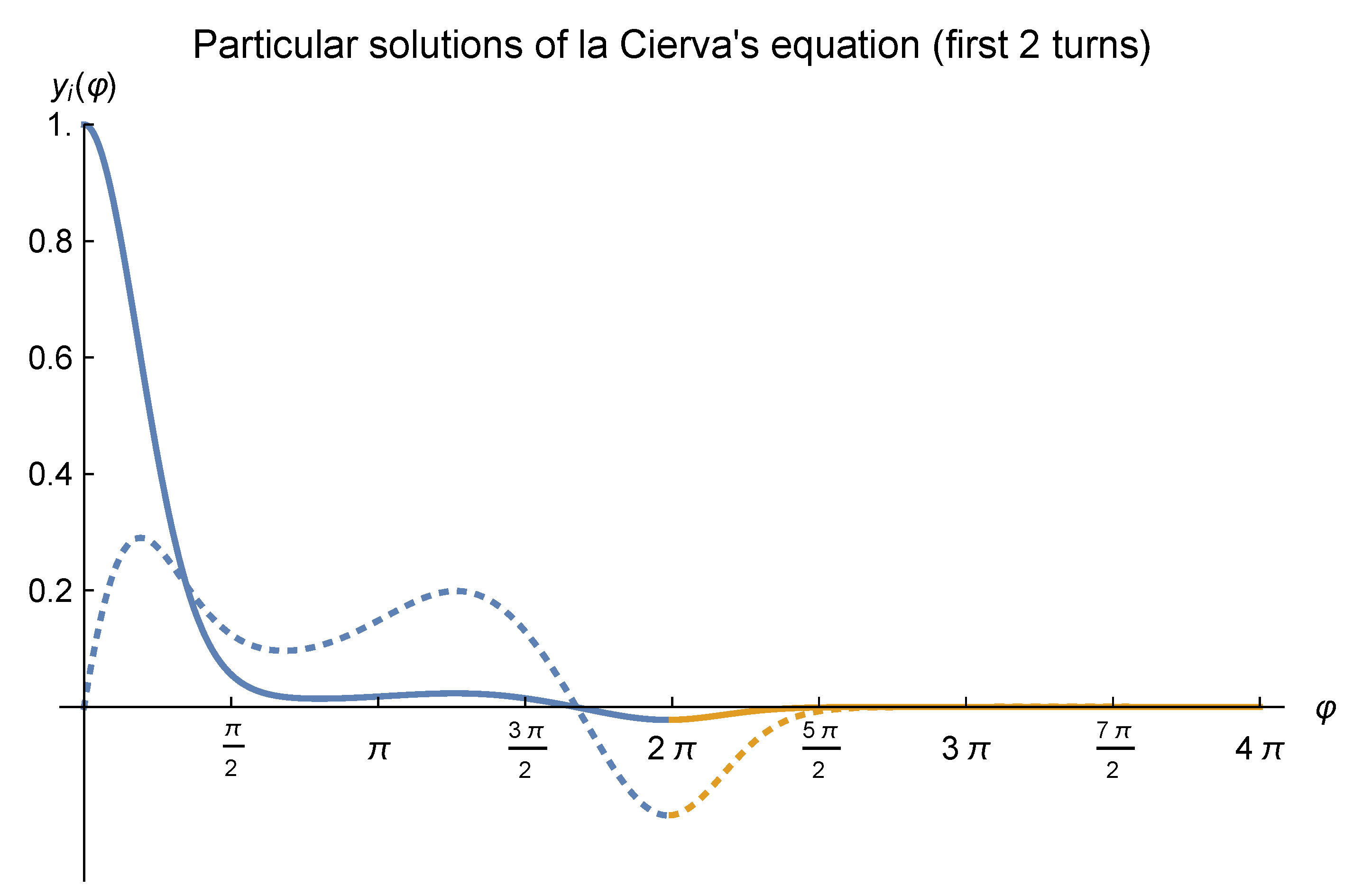
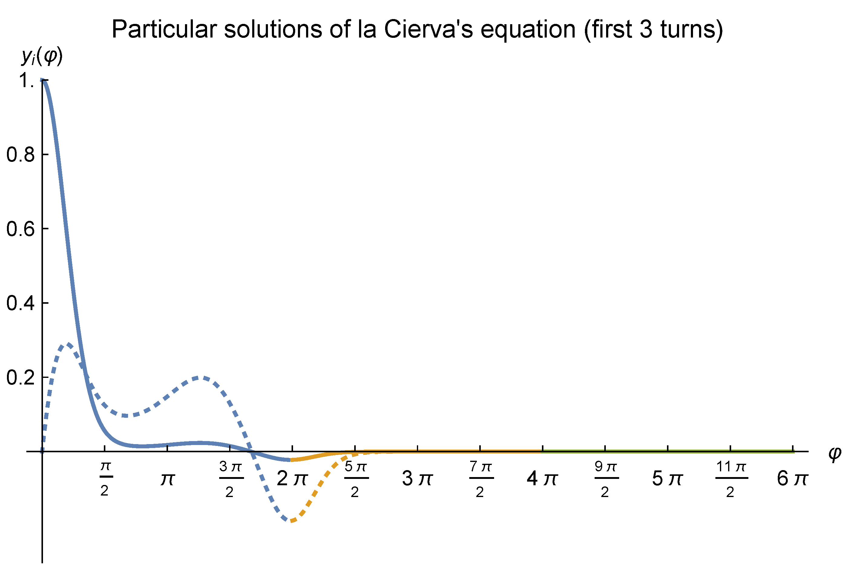
• In [7], Puig-Adam posed to analyze the area of the plane $\lambda -m$ where la Cierva’s equation becomes stable. To deal with, we considered the rectangle of the Euclidean plane, $R=[0,1]\times [0.15,1]$, by taking into account the intervals proposed by Mr. la Cierva for each parameter. A partition consisting of 50 points was considered for each subinterval, thus leading to a $2500—$point mesh contained in R. As such, for each $(\lambda ,m)\in R$, a la Cierva’s type equation (c.f. Equation (49)) holds, which was numerically solved as in Section 5 by means of the midpoint approach. Next step was to apply the Puig-Adam criterion to determine whether that equation is stable. Recall that such a condition consists of calculating $|y_1\left(2\pi \right)+y_2^{\prime }\left(2\pi \right)|$, where $y_1$ and $y_2$ denote the particular solutions of the corresponding la Cierva’s equation for a choice of parameters. If $k_{\lambda ,m}:=|y_1\left(2\pi \right)+y_2^{\prime }\left(2\pi \right)|<1$, then the la Cierva’s equation is stable for those parameters. All the above allowed us to construct a 3D-surface, $S=\{(\lambda ,m,k_{\lambda ,m}):(\lambda ,m)\in R\}$, we shall refer to as la Cierva’s surface. Figure 8 depicts la Cierva’s surface, whereas Figure 9 displays the contours of la Cierva’s surface. Such figures reveal an overall stable behavior of almost all la Cierva’s surface. On the other hand, Figure 10 and Figure 11 depict a neighborhood of Puig-Adam’s choice of parameters where la Cierva’s surface behaves stably, as stated in remark (5).
  

  Figure 8. La Cierva’s surface, $S=\{(\lambda ,m,k_{\lambda ,m}):(\lambda ,m)\in R\}$, where $R=[0,1]\times [0.15,1]$ (above). The plane $\left\{\right(\lambda ,m,1):(\lambda ,m)\in R\}$ has been graphically displayed as a benchmark regarding the limit of the stability zone for la Cierva’s surface (below).
  

  Figure 9. Contours of la Cierva’s surface. Observe that the Puig-Adam’s choice of parameters, $\lambda =1,m=0.5$ is indeed surrounded by a region of points with low $k_{\lambda ,m}$ numbers. Notice that almost all the whole surface behaves stably.
  

  Figure 10. A neighborhood of the Puig-Adam’s choice of parameters where la Cierva’s surface is stable.
  

  Figure 11. Contours of a neighborhood of the Puig-Adam’s choice of parameters where la Cierva’s surface behaves stably.

References

- Johnson, W. Helicopter Theory; Dover Publications, Inc.: Mineola, NY, USA, 1994. [Google Scholar]
- List of NASA Aircraft. 2020. Available online: https://en.wikipedia.org/wiki/List_of_NASA_aircraft (accessed on 16 October 2020).
- Machado, J.T.; Galhano, A.M. A fractional calculus perspective of distributed propeller design. Commun. Nonlinear Sci. Numer. Simul. 2018, 55, 174–182. [Google Scholar] [CrossRef]
- Bing, L.; Ning, Y.; YeHong, D. LAV Path Planning by Enhanced Fireworks Algorithm on Prior Knowledge. Appl. Math. Nonlinear Sci. 2016, 1, 65–78. [Google Scholar] [CrossRef]
- Zhang, Q. Fully discrete convergence analysis of non-linear hyperbolic equations based on finite element analysis. Appl. Math. Nonlinear Sci. 2019, 4, 433–444. [Google Scholar] [CrossRef]
- Herrera, E. Sin Alas ni Timones; Madrid Científico: Madrid, Spain, 1934; pp. 51–53. [Google Scholar]
- Puig-Adam, P. Sobre la estabilidad del movimiento de las palas del autogiro. Rev. Aeronaut. 1934, 30, 478–485. [Google Scholar]
- Orts y Aracil, J.M. Nota sobre la ecuación diferencial que plantea la estabilidad del autogiro ultrarrápido. Ibérica 1934, 1024, 295–296. [Google Scholar]
- Orts y Aracil, J.M. Nueva contribución al estudio del problema matemático del autogiro ultrarrápido. Ibérica 1934, 1029, 376–377. [Google Scholar]
- Liapounov, A.M. Problème général de la stabilité du mouvement. Ann. Fac. Sci. Toulouse 1903, 2, 203–474. [Google Scholar] [CrossRef]
- Goursat, E. Differential Equations. In A Course in Mathematical Analysis; Hedrick, E.R., Dunkel, O., Eds.; Ginn and Company: Boston, MA, USA, 1905; Volume II. [Google Scholar]
Publisher’s Note: MDPI stays neutral with regard to jurisdictional claims in published maps and institutional affiliations. |
© 2020 by the authors. Licensee MDPI, Basel, Switzerland. This article is an open access article distributed under the terms and conditions of the Creative Commons Attribution (CC BY) license (http://creativecommons.org/licenses/by/4.0/).