On the Entropy of Fractionally Integrated Gauss–Markov Processes

Abstract

This paper is devoted to the estimation of the entropy of the dynamical system $\{X_{\alpha }\left(t\right),t\ge 0\}$, where the stochastic process $X_{\alpha }\left(t\right)$ consists of the fractional Riemann–Liouville integral of order $\alpha \in (0,1)$ of a Gauss–Markov process. The study is based on a specific algorithm suitably devised in order to perform the simulation of sample paths of such processes and to evaluate the numerical approximation of the entropy. We focus on fractionally integrated Brownian motion and Ornstein–Uhlenbeck process due their main rule in the theory and application fields. Their entropy is specifically estimated by computing its approximation (ApEn). We investigate the relation between the value of $\alpha$ and the complexity degree; we show that the entropy of $X_{\alpha }\left(t\right)$ is a decreasing function of $\alpha \in (0,1)$.

1. Introduction

In the study of a biological system, whose time evolution is modeled by a stochastic process that depends on a certain parameter $\alpha ,$ often there is a need to find how a change in the value of $\alpha$ affects the qualitative behavior of the system, as well as its complexity degree, or entropy. Another useful information is the knowledge of a stochastic ordering, with respect to expectation of functionals of the process (e.g., its mean and variance), when varying $\alpha .$

As a case study, we are interested to the qualitative behavior of the fractional integral of a Gauss–Markov (GM) process, when varying the order $\alpha$ of the fractional integration.

Actually, GM processes and their fractional integrals over time are very relevant in various application fields, especially in Biology—e.g., in stochastic models for neuronal activity (see [1]). In particular, the fractional integral of order $\alpha \in (0,1)$ of a GM process, say $X_{\alpha }\left(t\right)$, is suitable to describe certain stochastic phenomena with long range memory dynamics, involving correlated input processes (see [2]).

As an example of application, one can consider the model for the neuronal activity, based on the coupled differential equations:

$$\begin{array}{c}\hfill \left\{\begin{array}{cc}{\mathcal{D}}^{\alpha }V\left(t\right)=\frac{g_L}{C_m}{V}_L+\frac{\eta \left(t\right)}{C_m},\hfill & V\left(0\right)=V_0\hfill \\ d\eta \left(t\right)=-\frac{\eta \left(t\right)-I\left(t\right)}{\tau }dt+\frac{\varsigma }{\tau }dB\left(t\right),\hfill & \eta \left(0\right)={\eta }_0.\hfill \end{array}\right.\end{array}$$

(1)

Here, ${\mathcal{D}}^{\alpha }$ stands for the Caputo fractional derivative (see [3]); $\eta \left(t\right)$ is in place of the white noise, usually utilized in the stochastic differential equation, which describes a Leaky Integrate-and-Fire (LIF) neuronal model (see, for example, [4]). The colored noise process $\eta \left(t\right)$ is the correlated process obeying the second of Equation (1) and it is the input for the first one; it is indeed a time-non-homogeneous GM process of Ornstein–Uhlenbeck (OU)-type (see Section 2). The stochastic process $V\left(t\right)$ represents the voltage of the neuronal membrane, whereas $C_m$ is the membrane capacitance, $g_L$ the leak conductance, $V_L$ the resting (equilibrium) level potential, $I\left(t\right)$ the synaptic current (deterministic function), $\tau$ is the correlation time of $\eta \left(t\right)$ and $B\left(t\right)$ the noise (standard BM). As we can see, the process $V\left(t\right)$, which is the solution of (1) belongs to the class of fractional integrals of GM processes. Indeed, it is a specific example of $X_{\alpha }\left(t\right)$ process, $V\left(t\right)$ being the Caputo fractional integral of the $\eta \left(t\right)$ process [5]. The biophysical motivation in the above model is to describe a neuronal activity as a perfect integrator (without leakage), from an initial time until to the current time, of the process $\eta \left(t\right)$, representing the time dependent input. The use of fractional operators allows us to regulate the time scale by choosing the fractional order of integration suitably adherent to the neuro-physiological evidences. Indeed, such a model can be useful, for instance, in the investigation and simulation of synchronous/asynchronous communications in networks of neurons [6].

To introduce the terms of our investigation, we recall some definitions.

A continuous GM process $Y\left(t\right)$ is a stochastic process of the form:

$$Y\left(t\right)=m\left(t\right)+h_2\left(t\right)B\left(r\left(t\right)\right),t\ge 0,$$

(2)

where $B\left(t\right)=B_t$ denotes standard Brownian motion (BM), $m\left(t\right),h_1\left(t\right),h_2\left(t\right)$ are $C^1$ functions in $(0,+\infty ),$ with $h_2\left(t\right)\ne 0$ and $r\left(t\right)=h_1\left(t\right)/h_2\left(t\right)$ is a monotone increasing, differentiable and non-negative function.

For a continuous function $f\left(t\right),$ its Riemann–Liouville (RL) fractional integral of order $\alpha \in (0,1)$ is defined as (see [7]):

$${\mathcal{I}}^{\alpha }\left(f\right)\left(t\right)=\frac{1}{\Gamma \left(\alpha \right)}{\int }_0^t{(t-s)}^{\alpha -1}f\left(s\right)ds,$$

(3)

where $\Gamma$ is the Gamma Euler function—i.e., $\Gamma \left(z\right)={\int }_0^{+\infty }{t}^{z-1}{e}^{-t}dt,z>0.$

We recall also that the Caputo fractional derivative of order $\alpha$ of a function $f\left(t\right)$ is defined by (see [3]):

$${\mathcal{D}}^{\alpha }f\left(t\right)=\frac{1}{\Gamma (1-\alpha )}{\int }_0^t\frac{f^{\prime }\left(s\right)}{{(t-s)}^{\alpha }}ds,$$

(4)

where $f^{\prime }$ denotes the ordinary derivative of $f.$

Notice that, taking the limit for $\alpha \to 1,$ one gets ${\mathcal{D}}^{1}f\left(t\right)=f^{\prime }\left(t\right),$ while ${\mathcal{I}}^1\left(f\right)\left(t\right)={\int }_0^{t}f\left(s\right)ds$—i.e., the ordinary Riemann integral of f. Moreover, ${\mathcal{D}}^{0}f\left(t\right)=f\left(t\right)-f\left(0\right)$ and ${\mathcal{I}}^0\left(f\right)\left(t\right)=f\left(t\right).$

Referring to the neuronal model (1), assuming that $V\left(0\right)=0$ (and, in some cases, also $\eta \left(0\right)=0$), the RL fractional integral ${\mathcal{I}}^{\alpha }$ is used as the left-inverse of the Caputo derivative ${\mathcal{D}}^{\alpha }$ (see [8,9]). In this way, we find that the solution $V\left(t\right)$ of (1) involves the RL fractional integral process of the GM process $\eta \left(t\right),$ specifically:

$$V\left(t\right)={\mathcal{I}}^{\alpha }\left({\mathcal{D}}^{\alpha }V\left(t\right)\right)={\mathcal{I}}^{\alpha }\left(\frac{g_L}{C_m}{V}_L\right)+{\mathcal{I}}^{\alpha }\left(\frac{\eta \left(t\right)}{C_m}\right),\mathrm{with}V\left(0\right)=0.$$

(5)

Thus, $V\left(t\right)$ turns out to be written in terms of the fractional integral of $\eta \left(t\right).$

From this consideration, in the framework of general stochastic models involving correlated processes, it appears useful to investigate the properties of $X_{\alpha }\left(t\right)={\mathcal{I}}^{\alpha }\left(Y\right)\left(t\right),$—i.e., the fractional integral of a GM process $Y\left(t\right),$ as varying $\alpha \in (0,1).$ Although $X_{\alpha }\left(t\right)$ is not Markov, we have showed in [2] that it is still a Gaussian process with mean ${\mu }_{\alpha }\left(t\right)$ and variance ${\sigma }_{\alpha }^2\left(t\right);$ for instance, the fractional integral of BM has mean ${\mu }_{\alpha }\left(t\right)=0$ and variance

$${\sigma }_{\alpha }^2\left(t\right)=\frac{t^{2\alpha +1}}{(2\alpha +1){\Gamma }^2(\alpha +1)}$$

(for closed formulae of the mean ${\mu }_{\alpha }\left(t\right)$ and variance ${\sigma }_{\alpha }^2\left(t\right)$ of the fractional integral of a general GM process, see [2]). For fixed $\alpha ,{\sigma }_{\alpha }^2\left(t\right)$ turned out to be increasing, as a function of $t.$ Moreover, in [2] we found that for small values of time t the variances of the considered fractionally integrated GM processes become ever lower, as $\alpha$ increases (i.e., the variance decreases as a function of $\alpha );$ for large values of t this behavior is overturned, and the variance increases with $\alpha$ (see [2]).

In this paper, we aim to characterize the qualitative behavior of the dynamical system $X_{\alpha }\left(t\right),\alpha \in (0,1)$ by means of its entropy. Indeed, the entropy is widely used for this purpose in many fields (see [10,11,12,13,14]). In Biology, entropy is useful to characterize the behavior of, for example, Leaky Integrate-and-Fire (LIF) neuronal models (see [4]). In finance, Kelly in [15] introduced entropy for gambling on horse races, and Breiman in [16] for investments in general markets. Finally, the admissible self-financing strategy achieving the maximum entropy results in a growth optimal strategy (see [17]).

In order to specify the entropy for the processes considered in this paper, we first note that, for a fixed time s the r.v. $X_{\alpha }\left(s\right)$ is normally distributed with mean ${\mu }_{\alpha }\left(s\right)$ and variance ${\sigma }_{\alpha }^2\left(s\right)$, so recalling that the entropy of a r.v. X with density $f\left(x\right)$ is given by

$$H\left(X\right)=-{\int }_{-\infty }^{+\infty }{log}_2\left(f\left(x\right)\right)f\left(x\right)dx,$$

(6)

where, by calculation, it easily follows that the entropy of the normal r.v. $X=X_{\alpha }\left(s\right)$ with fixed $s,$ depends only on ${\sigma }_{\alpha }^2\left(s\right)$ and it is given by (see [18], p. 181):

$$H\left(X\right)={log}_2\left({\sigma }_{\alpha }\left(s\right)\sqrt{2\pi e}\right).$$

(7)

Thus, the larger the variance ${\sigma }_{\alpha }^2\left(s\right),$ the larger the entropy of $X_{\alpha }\left(s\right)$ for a fixed time $s.$

In this paper we are interested in studying a different quantity: for a certain value of $\alpha \in (0,1),$ and $T>0$, our aim is to find the entropy of trajectories of $X_{\alpha }\left(t\right),t\in [0,T],$ which involves all the points of the trajectories up to time $T,$ and to show that the entropy is a decreasing function of $\alpha .$

We do not actually compute the entropy of $X_{\alpha }\left(t\right),$ but its approximate entropy ApEn (see [19]), obtained by using several long enough simulated trajectories (they were previously obtained in [2], for the fractional integral of some noteworthy GM processes $Y\left(t\right)$, namely, BM and Ornstein–Uhlenbeck (OU)). In fact, Pincus [19] has showed that ApEn is suitable to quantify the concept of changing complexity, being able to distinguish a wide variety of system behaviors. Indeed, for general time series, it can potentially separate those coming from deterministic systems and stochastic ones, and those coming from periodic systems and chaotic ones; moreover, for a homogeneous, ergodic Markov chain, ApEn coincides with Kolmogorov–Sinai entropy. Thus, though $X_{\alpha }\left(t\right)$ is not a Markov process, its approximate entropy ApEn is able to characterize the complexity degree of the system, when varying $\alpha .$

As we said, we previously found that, in all the considered cases of GM processes, for large t the variance ${\sigma }_{\alpha }^2\left(t\right)$ of their fractional integral $X_{\alpha }\left(t\right)$ is an increasing function of $\alpha ,$ while for small t it decreases with $\alpha ;$ instead, the covariance function has more diversified behaviors (see [2]).

In the present article, we show that, for small values of $\alpha \in (0,1),X_{\alpha }\left(t\right)$ exhibits a large value of the complexity degree; a possible explanation is that, for small $\alpha$ the trajectories of the process $X_{\alpha }\left(t\right)$ become more jagged, giving rise to a greater value of the complexity degree. In fact, our estimates of ApEn show that it is a decreasing function of $\alpha \in (0,1).$ This behavior appears for the fractional integral of BM (FIBM), as well as for the fractional integral of the OU process (FIOU).

2. The Entropy of the Trajectories of ${\mathit{X}}_{\mathit{\alpha }}\left(\mathit{t}\right)$

In this section, we study the complexity degree of the trajectories of the process $X_{\alpha }\left(t\right)$, in two noteworthy cases of GM processes $Y\left(t\right),$ precisely:

(i)

$Y\left(t\right)=B_t,$ so $X_{\alpha }\left(t\right)={\mathcal{I}}^{\alpha }\left(B\right)\left(t\right)$ is fractionally integrated Brownian motion (FIBM);

(ii)

$Y\left(t\right)$ is the Ornstein–Uhlenbeck (OU) process, driven by the SDE.

$$dY\left(t\right)=-(\mu Y\left(t\right)-\beta )dt+\sigma d{B}_t,Y\left(0\right)=y(\mu ,\sigma >0,\beta \in \mathbb{R}),$$

(8)

which can be expressed as (see [20]):

$$Y\left(t\right)=\beta +e^{-\mu t}[y-\beta +B\left(r\left(t\right)\right)],$$

(9)

where the equality is meant in distribution, and

$$r\left(t\right)=\frac{{\sigma }^2}{2\mu }\left(e^{2\mu t}-1\right).$$

(10)

OU process $Y\left(t\right)$ is a GM process of the form (2), with:

$$m\left(t\right)=\beta +e^{-\mu t}(y-\beta ),h_1\left(t\right)=\frac{{\sigma }^2}{2\mu }\left(e^{\mu t}-e^{-\mu t}\right),h_2\left(t\right)=e^{-\mu t},$$

(11)

and covariance

$$c(s,t)=h_1\left(s\right)h_2\left(t\right)=\frac{{\sigma }^2}{2\mu }\left(e^{-\mu (t-s)}-e^{-\mu (s+t)}\right),0\le s\le t.$$

(12)

Then, $X_{\alpha }\left(t\right)={\mathcal{I}}^{\alpha }\left(Y\right)\left(t\right)$ is called the fractionally integrated OU (FIOU) process.

Both FIBM and FIOU are Gaussian processes whose variance and covariance functions were explicitly obtained in [2] and studied, as functions of $\alpha \in (0,1).$

To study the complexity degree of the trajectories of the process $X_{\alpha }\left(t\right)$, in cases (i) and (ii), we make use of several simulated trajectories of length $N,$ previously obtained in [2], for N large. The sample paths have been obtained by using the R software, with time discretization step $h=0.01$ and by means of the same sequence of pseudo-random Gaussian numbers. The simulation algorithm has been realized as an R script. More specifically, we specialize the algorithm to simulate an array of $(x_1,x_2,\dots ,x_N)$ Gaussian numbers with a specified covariance matrix. Indeed, we first set the time instants $t_1<t_2<\dots <t_N$ (with $t_0=0$ and $t_i=t_{i-1}+h,i=1,\dots ,N)$ and we evaluate the elements of the covariance matrix $C_{i,j}=cov(X_{\alpha }\left(t_i\right),X_{\alpha }\left(t_j\right)).$ Note that, for each fractionally integrated Gauss–Markov process here considered, we implemented a specific algorithm to be evaluated by numerical procedures the mathematical expression of the covariance according to Equation (3.5) of [2]. Then, we apply the Cholesky decomposition to matrix C in order to determine the lower triangular matrix G, such that $C=G{G}^T$, where $G^T$ is the transposition of $G.$ Finally, we generate N pseudo-Gaussian standard numbers $(z_1,z_2,\dots ,z_N)\equiv {\mathbf{z}}^{\mathbf{T}}$ and we set $x_i=G_i\mathbf{z}$ (for $i=1,\dots ,N$, with $G_i$ the $i-$th row of matrix G) such that the obtained array $(x_1,x_2,\dots ,x_N)$ is a simulation of a centered Gaussian distributed N-dimensional r.v. with covariances $cov(x_i,x_j)=C_{i,j}$ for $i,j=1,\dots ,N.$

In particular, referring to algorithms for the generation of pseudo-random numbers (see [21]), the main steps of implementation were the following (for more, see [2]):

STEP 1

The elements of $N\times N$ covariance matrix $C(t_i,t_j)$ are calculated at times $t_i,i=1,\dots ,N,$ of an equi-spaced temporal grid.

STEP 2

The Cholesky decomposition algorithm is applied to the covariance matrix C in order to obtain a lower triangular matrix $G(i,j)$, such that $C=G{G}^T.$

STEP 3

The N-dimensional array $\mathbf{z}$ of standard pseudo-Gaussian numbers is generated.

STEP 4

The sequence of simulated values of the correlated fractionally integrated process is constructed as the array $\mathbf{x}=G\mathbf{z}.$

Finally, the array $\mathbf{x}$ provides the simulated path—i.e., a realization $(x_1,x_2,\dots ,x_N),$ of $(X_{\alpha }\left(t_1\right),\dots ,X_{\alpha }\left(t_N\right)),$ whose components have the assigned covariance.

2.1. The Approximate Entropy

In [19] Pincus defined the concept of approximate entropy (ApEn) to measure the complexity of a system, proving also that, for a Markov chain, ApEn equals the entropy rate of the chain. In fact, to measure chaos concerning a given set of data, we have at our disposal Hausdorff and correlation dimension, K-S entropy, and the Lyapunov spectrum (see [19]); indeed, to calculate one of the above parameters, one needs an impractically large amount of data. Instead, calculation of ApEn(m, r) (see below for the definition) only requires relatively few points. Actually, as shown in [19], if one uses only 1000 points, and m is taken as being equal to 2, ApEn(m, r) can characterize a large variety of system behaviors, since it is able to distinguish deterministic systems from stochastic ones, and periodic systems from chaotic ones.

For instance, Abundo et al. [10] used ApEn to obtain numerical approximations of the entropy rate, with the final purpose to investigate the degree of cooperativity of proteins in a Markov model with binomial transition distributions. They showed that the corresponding ApEn is a decreasing function of the degree of cooperativity (for more about approximation of entropy by numerical algorithms, see [12] and references therein).

Now, we recall from [19] the definition of ApEn. Let $\{x_1,x_2,...,x_N\}$ be given a time-series of data, equally spaced in time, and fix an integer $m>0$ and a positive number $r.$ Next, let us consider a sequence of vectors $\{{\underline{v}}_1,{\underline{v}}_2,...,{\underline{v}}_{N-m+1}\}$ in ${\mathbb{R}}^m$ defined by ${\underline{v}}_i=(x_i,x_{i+1},...,x_{i+m-1}).$ Then, define for each i, $1\le i\le N-m+1,$

$${\mathcal{C}}_i(m,r)=\frac{\#ofjsuchthatd({\underline{v}}_i,{\underline{v}}_j)\le r}{N-m+1},$$

(13)

in which the distance $d(·,·)$ between two vectors is defined by

$$d({\underline{v}}_i,{\underline{v}}_j)=\underset{k=1,...,m}{max}|x_{i+k-1}-x_{j+k-1}|.$$

(14)

We observe that the ${\mathcal{C}}_i(m,r)$ quantities measure up to a tolerance r the frequency of patterns which are similar to a certain pattern whose window length is $m.$ Now, define

$${\Phi }_N(m,r)=\frac{{\sum }_{i=1}^{N-m+1}log{\mathcal{C}}_i(m,r)}{N-m+1}$$

(15)

and

$$ApEn(m,r)=\underset{N\to \infty }{lim}({\Phi }_N(m,r)-{\Phi }_N(m+1,r)).$$

(16)

Given N data points, formula (16) can be implemented by defining the statistics

$$\widehat{ApEn}(m,r,N)={\Phi }_N(m,r)-{\Phi }_N(m+1,r).$$

(17)

Heuristically, we can say that ApEn is a measure of the logarithmic likelihood that runs of patterns that are close for m observations, remain close on the next incremental comparison. A greater likelihood of remaining close (i.e., regularity) produces smaller ApEn values, and viceversa. On the basis of simulated data, Pincus showed that, for $N=1000$ and $m=2$, for values of r, between $0.1$ and $0.2$ times the standard deviation of the $x_i$ data produce reasonable statistical validity of $\widehat{ApEn}(m,r,N).$ Moreover, he showed that, for a homogeneous, ergodic Markov chain, ApEn coincides with the Kolmogorov–Sinai entropy (see [14]), that is

$$ApEn(m,r)=-\sum _i\sum _j{\pi }_i{p}_{ij}log{p}_{ij},$$

where $p_{ij}$ denotes the transition probability of the Markov chain from the state i to the state j, and ${\pi }_j={lim}_{n\to \infty }{p}_{ij}^{\left(n\right)}$ is the $j-$th component of the vector $\pi =({\pi }_1,{\pi }_2,\cdots )$ of the stationary probabilities, being $p_{ij}^{\left(n\right)}$ the $n-$step transition probability of the Markov chain from the state i to the state j.

2.2. Calculation of the Entropy of Simulated Trajectories of the Process $X_{\alpha }\left(t\right)$

In the case of FIBM and FIOU, for a set of values $\alpha \in (0,1),$ we have performed L (discretized) trajectories $(x_1,x_2,\dots ,x_N)$ of length N of the process $X_{\alpha }\left(t\right),$ by means of the simulation algorithm previously described in STEPS 1–4. In particular, for each simulated path, we follow the remaining steps:

STEP 5

Construction of the array $\{{\underline{v}}_{1,\alpha },{\underline{v}}_{2,\alpha },...,{\underline{v}}_{N-m+1,\alpha }\}$ in ${\mathbb{R}}^m$ (for a fixed m) by extracting from a given sample path $(x_1,x_2,\dots ,x_N)\equiv (X_{\alpha }\left(t_1\right),...,X_{\alpha }\left(t_N\right))$, obtained in STEPS 1–4, the vectors ${\underline{v}}_{i,\alpha }=(X_{\alpha }\left(t_i\right),X_{\alpha }\left(t_{i+1}\right),...,X_{\alpha }\left(t_{i+m-1}\right)).$

STEP 6

Construction of the distance matrix $D_{i,j}^{\alpha }$ whose elements are $d_{i,j}^{\alpha }$ are defined as the follows distance between vectors $v_{i,\alpha }$ and ${\underline{v}}_{j,\alpha }$—i.e.,

$$d_{i,j}^{\alpha }=d({\underline{v}}_{i,\alpha },{\underline{v}}_{j,\alpha })=\underset{k=1,...,m}{max}|X_{\alpha }\left(t_{i+k-1}\right)-X_{\alpha }\left(t_{j+k-1}\right)|.$$

(18)

STEP 7

After setting $r=0.1\ast \mathcal{S}$, with $\mathcal{S}$ sample deviation of simulated paths, evaluation of array ${\mathcal{C}}^{\alpha }$ whose components are provided as

$${\mathcal{C}}_i^{\alpha }=\frac{\#ofjsuchthatd({\underline{v}}_{i,\alpha },{\underline{v}}_{j,\alpha })\le r}{N-m+1},$$

(19)

for $1\le i\le N-m+1.$

STEP 8

Evaluation of the quantities

$${\Phi }_{N,m}^{\alpha }=\frac{{\sum }_{i=1}^{N-m+1}log{\mathcal{C}}_i^{\alpha }}{N-m+1},{\Phi }_{N,m+1}^{\alpha }=\frac{{\sum }_{i=1}^{N-m}log{\mathcal{C}}_i^{\alpha }}{N-m}$$

(20)

and

$${ApEn}_{\alpha }={\Phi }_{N,m}^{\alpha }-{\Phi }_{N,m+1}^{\alpha }.$$

(21)

We have taken the number of paths L large enough and N from 100 to $300,$ and for each of these L trajectories of length $N,$ corresponding to a value of $\alpha ,$ we have estimated ${ApEn}_{\alpha }\left(i\right),i=1,\dots ,L$ by means of the approximation $\widehat{ApEn}(2,r,N),$ where $r=0.1\times$ (the standard deviation of trajectory points); then, the approximate entropy of $X_{\alpha }\left(t\right)$ has been obtained by ${ApEn}_{\alpha }^L=\frac{1}{L}{\sum }_{i=1}^L{ApEn}_{\alpha }\left(i\right).$ This allowed us to study the dependence of the entropy of the sample paths of $X_{\alpha }\left(t\right)={\mathcal{I}}^{\alpha }\left(Y\right)\left(t\right)$ on the parameter $\alpha ,$ showing that the entropy—namely a measure of the complexity of the dynamical system $X_{\alpha }\left(t\right)$—is a decreasing function of $\alpha \in (0,1).$

Since the fractional integral of order zero of $Y\left(t\right)$ is nothing but the process $Y\left(t\right)$ itself, and the fractional integral of order 1 is the ordinary Riemann integral of $Y\left(t\right),$ our result means that fractional integration introduces a greater degree of complexity than that corresponding to ordinary integration; moreover, the maximum degree of complexity is obtained for the original process $Y\left(t\right)$ (that is, without integration).

In Figure 1 and Figure 2 we plot the numerical results for ApEn, as a function of $\alpha ,$ for FIBM and FIOU, respectively. When the estimates of ApEn have been obtained for $N=100,$ it appears clear that ApEn is a decreasing function of $\alpha .$

Figure 1. Approximate entropy (ApEn) of FIBM, as a function of $\alpha$ for $N=100.$ (Values of $\alpha$ are on the horizontal axes).

Figure 2. Approximate entropy (ApEn) of FIOU with $\mu =\sigma =1,\beta =0,$ as a function of $\alpha$ for $N=100.$ (Values of $\alpha$ are on the horizontal axes).

Moreover, our calculation highlights that, for small values of $\alpha$, the trajectories of FIBM and FIOU become more jagged, giving rise to a greater value of the complexity degree (see Figure 3).

Figure 3. Some simulated sample paths of FIBM (left) and of FIOU (right) for some values of $\alpha$ (specified by labels inside the figure). In both examples we set $N=100$, but the time discretization step h is $0.01$ on the left and $0.1$ on the right. The seed of the random generator is the same for all simulated paths. (Values of time t are on the horizontal axes).

We also show that the results of ApEn as N increases in Figure 4 and Figure 5. Our investigations show that the estimated values of ApEn for FIOU, for a given $\alpha$ and a given trajectory length, are considerably larger than those for FIBM (compare Figure 4 and Figure 5). This possibly depends on the fact that the trajectories of FIOU are more complicated than those of FIBM, giving rise to a greater complexity degree. Moreover, contrary to the case of FIBM, where for all $\alpha$ the estimated value of ApEn is a decreasing function of the length N of simulated trajectories, in the case of FIOU, for $\alpha \le 0.5$, the estimated value of ApEn appears to be an increasing function of $N.$ Perhaps if one used far longer trajectories $(N\ge 1000)$ to estimate ApEn, the values obtained in both cases would be comparable and they would exhibit the same behavior as a function of $N.$ Notice, however, that to simulate very long trajectories is impractical from the computational point of view (even for $N=300$, the CPU time to evaluate ApEn in the case of FIOU was of order of almost one hour).

Figure 4. Approximate entropy (ApEn) of FIBM, for various value of $\alpha$ (specified by labels inside the figure) and N (on the horizontal axes).

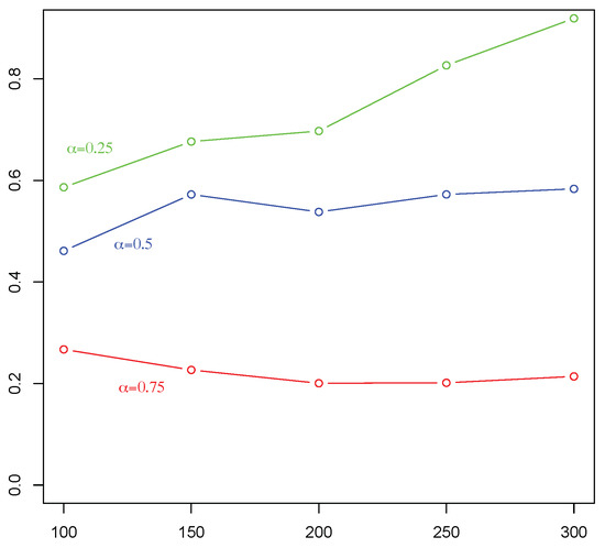
Figure 5. Approximate entropy (ApEn) of FIOU with $\mu =\sigma =1,\beta =0,$ for various value of $\alpha$ (specified by labels inside the figure) and N (on the horizontal axes).

3. Conclusions and Final Remarks

In this paper, we further investigated the qualitative behavior of the fractional integral of order $\alpha \in (0,1)$ of a Gauss–Markov process, that we already studied in [2].

Actually, Gauss–Markov processes and their fractional integrals over time are very relevant in various application fields, especially in Biology—e.g., in stochastic models for neuronal activity (see [1]). In fact, the fractional integral of order $\alpha \in (0,1)$ of a Gauss–Markov process $Y\left(t\right)$, say $X_{\alpha }\left(t\right),$ is suitable to describe stochastic phenomena with long range memory dynamics, involving correlated input processes, which are very relevant in Biology (see [2]).

While in [2] we have showed that $X_{\alpha }\left(t\right)$ is itself a Gaussian process, and we have found its variance and covariance, obtaining that the variance ${\sigma }_{\alpha }^2\left(t\right)$ of $X_{\alpha }\left(t\right)$ is an increasing function of $\alpha ,$ in this paper we have characterized the qualitative behavior of the dynamical system $X_{\alpha }\left(t\right),\alpha \in (0,1)$ by means of its complexity degree, or entropy. Actually, for several values of $\alpha$ we have estimated its approximate entropy ApEn, obtained by long enough trajectories of the process $X_{\alpha }\left(t\right).$ Specifically, we investigate the problem by means of the implementation of an algorithm based on STEPS 1–8 detailed described in the paper. We have found that ApEn is a decreasing function of $\alpha ;$ this behavior appeared for the fractional integral of the Brownian motion, as well as for the fractional integral of Ornstein–Uhlenbeck process. Since the fractional integral of $Y\left(t\right)$ of order zero is nothing but the process $Y\left(t\right)$ itself, and the fractional integral of order 1 is the Riemann integral of $Y\left(t\right),$ our result means that fractional integration introduces a greater degree of complexity than in the case of ordinary integration; moreover, the maximum degree of complexity is obtained for the original Gauss–Markov process $Y\left(t\right)$ (that is, without integration).

Furthermore, we remark that the algorithm for computing ApEn uses numerical data, which can be used independently of knowing the process where they come from. However, in our case, we study the process $X_{\alpha }\left(t\right),$ when varying the parameter $\alpha ,$ so we need to simulate its trajectories, and to make use of the obtained numerical values to estimate ApEn. As regards the possibility of finding out, by using ApEn, if certain data come from a particular class of possible systems, we have not investigated this. Our aim was only to characterize the behavior of fractionally integrated Gauss–Markov process $X_{\alpha }\left(t\right),$ as varying the parameter $\alpha ,$ by means of the corresponding value of ApEn.

As a future work, we aim to estimate the entropy for other cases of fractionally integrated Gauss–Markov processes $X_{\alpha }\left(t\right),$ such as the fractional integral of stationary Ornstein–Uhlenbeck process. Moreover, in order to further characterize the qualitative behavior of $X_{\alpha }\left(t\right)$ in terms of $\alpha ,$ our investigation will be addressed to estimate the fractal dimension of its trajectories, as a function of $\alpha .$

References

- Pirozzi, E. Colored noise and a stochastic fractional model for correlated inputs and adaptation in neuronal firing. Biol. Cybern. 2018, 112, 25–39. [Google Scholar] [CrossRef] [PubMed]
- Abundo, M.; Pirozzi, E. On the Fractional Riemann-Liouville Integral of Gauss-Markov processes and applications. arXiv 2019, arXiv:1905.08167. [Google Scholar]
- Caputo, M. Linear models of dissipation whose Q is almost frequency independent–II. Geophys. J. R. Astron. Soc. 1967, 13, 529–539. [Google Scholar] [CrossRef]
- Burkitt, A.N. A review of the integrate-and-fire neuron model: I. Homogeneous synaptic input. Biol. Cybern. 2006, 95, 1–19. [Google Scholar] [CrossRef] [PubMed]
- Pirozzi, E. On the Integration of Fractional Neuronal Dynamics Driven by Correlated Processes; Lecture Notes in Computer Science, 12013 LNCS; Springer: Cham, Switzerland, 2019; pp. 211–219. [Google Scholar]
- Tamura, S.; Nishitani, Y.; Hosokawa, C.; Mizuno-Matsumoto, Y. Asynchronous Multiplex Communication Channels in 2-D Neural Network with Fluctuating Characteristics. IEEE Trans. Neural Netw. Learn. Syst. 2018, 30, 2336–2345. [Google Scholar] [CrossRef] [PubMed]
- Debnath, L. Fractional integral and fractional differential equations in fluid mechanics. Fract. Calc. Appl. Anal. 2003, 6, 119–155. [Google Scholar]
- Kilbas, A.A.; Srivastava, H.M.; Trujillo, J.J. Theory and applications of fractional differential equations, volume 204. In North-Holland Mathematics Studies; Elsevier: Amsterdam, The Netherlands, 2006. [Google Scholar]
- Malinowska, A.B. Advanced Methods in the Fractional Calculus of Variations; Springer Briefs in Applied Sciences and Technology; Springer: Berlin/Heidelberg, Germany, 2015. [Google Scholar] [CrossRef]
- Abundo, M.; Accardi, L.; Rosato, N.; Stella, L. Analyzing protein energy data by a stochastic model for cooperative interactions: Comparison and characterization of cooperativity. J. Math. Biol. 2002, 44, 341–359. [Google Scholar] [CrossRef] [PubMed]
- Bollt, E.M.; Skufca, J.D. Control entropy: A complexity measure for nonstationary signals. Math. Biosci. Eng. 2009, 6. [Google Scholar] [CrossRef]
- Ciuperca, G.; Girardin, V. On the estimation of the entropy rate of finite Markov chains. In Proceedings of the International Symposium on Applied Stochastic Models and Data Analysis, Brest, France, 17–20 January 2005. [Google Scholar]
- Delgado-Bonal, A.; Marshak, A. Approximate Entropy and Sample Entropy: A Comprehensive Tutorial. Entropy 2019, 21, 541. [Google Scholar] [CrossRef]
- Walters, P. An Introduction to Ergodic Theory; Springer: New York, NY, USA, 1982. [Google Scholar]
- Kelly, J.L. A new interpretation for the information rate. Bell Syst. Tech. J. 1956, 35, 917–926. [Google Scholar] [CrossRef]
- Breiman, L. Optimal gambling system for favorable games. In Proceedings of the 4-th Berkeley Symposium on Mathematical Statistics and Probablity, Berkeley, CA, USA, 20 June–30 July 1960; University California Press: Cambridge, UK, 1960; Volume 1, pp. 65–78. [Google Scholar]
- Li, P.; Yan, J. The growth optimal portfolio in discrete-time financial markets. Adv. Math. 2002, 31, 537–542. [Google Scholar]
- Applebaum, D. Probability and Information; Cambridge University Press: Cambridge, UK, 2008. [Google Scholar]
- Pincus, S.M. Approximate entropy as a measure of system complexity. Proc. Natl. Acad. Sci. USA 1991, 88, 2297–2301. [Google Scholar] [CrossRef] [PubMed]
- Abundo, M. An inverse first-passage problem for one-dimensional diffusion with random starting point. Stat. Probab. Lett. 2012, 82, 7–14. [Google Scholar] [CrossRef]
- Haugh, M. Generating Random Variables and Stochastic Processes. In IEOR E4703: Monte Carlo Simulation; Columbia University: New York, NY, USA, 2016. [Google Scholar]
Publisher’s Note: MDPI stays neutral with regard to jurisdictional claims in published maps and institutional affiliations. |
© 2020 by the authors. Licensee MDPI, Basel, Switzerland. This article is an open access article distributed under the terms and conditions of the Creative Commons Attribution (CC BY) license (http://creativecommons.org/licenses/by/4.0/).