Dyadic Green’s Function and the Application of Two-Layer Model

Abstract

Dyadic Green’s function (DGF) is a powerful and elegant way of solving electromagnetic problems in the multilayered media. In this paper, we introduce the electric and magnetic DGFs in free space, respectively. Furthermore, the symmetry of different kinds of DGFs is proved. This paper focuses on the application of DGF in a two-layer model. By introducing the universal form of the vector wave functions in space rectangular, cylindrical and spherical coordinates, the corresponding DGFs are obtained. We derive the concise and explicit formulas for the electric fields represented by a vertical electric dipole source. It is expected that the proposed DGF can be extended to some more electric field problem in the two-layer model.

1. Introduction

Dyadic Green’s function (DGF) is one of the most useful mathematical tools in the application fields of electromagnetic field theory such as antennas and microwave remote sensing. The applications in the electromagnetic scattering have become more popular in recent years. This has prompted researchers to investigate different kinds of DGFs.

DGF plays a fundamental role in addressing the issue of integral equation method. The idea of DGF was first reported by Schwinger in 1950 [1] who used DGF method to deal with the boundary value problem of electromagnetic field. Since then, a great amount of work on DGF has been done, from unbounded free space [2] to half-space [3], from isotropic media [4] to anisotropic media [5], and from one and two-dimensional space [6] to three-dimensional space [7], Werner and Weiglhofer proposed analytic solutions to the differential equations for the DGFs, which are applicable to free space [8]. With the development of the volume integral equation, there have been increasing numerical methods studying the DGF in anisotropic and inhomogeneous media [9,10]. Frank and Ismo derived DGF for a new combined nonreciprocal and uniaxial bi-anisotropic medium [11]. Sihvola and Lindell investigated electromagnetic Green dyadic for unbounded bi-anisotropic media [12].

Because of the complexity of practical engineering, it is often necessary to use DGF to solve electromagnetic problems with different geometric structures. An analytic solution of electromagnetic-wave propagation in a rectangular waveguide has been investigated in terms of DGFs by Li et al. [13]. Kisliuk and Moshe also presented electric and magnetic fields generated by a given distribution of electric and magnetic currents in cylindrical waveguides [14]. Meanwhile, DGFs can also be used to analyze the scattering problems of complex geometric structures. For instance, chiral spheres [15], multiple cavities [16,17], a multilayered spherical media [18] and inhomogeneous ionospheric waveguides [19] have been investigated.

Several methods have been proposed to solve the DGF. Image method was applied to derive the DGF of a loaded rectangular waveguide in [20]. The DGF for an infinite perfect electromagnetic conductor cylinder has been given in [21] by using the principle of scattering superposition and the Ohm–Rayleigh method. Due to the widespread applications of the scattering in multi-layered media, there has been considerable research on DGF of multi-layered media. Yin and Wang investigated the radiation of cylindrical antennas over one and two-layer media [22]. Tamir [23] has established a three-layer forest model to study radio wave propagation in forests. Recently, DGF in two and three-layered medium model was proposed to obtain a propagation model of the typical Amazon city [24]. This paper is intended to develop a new method for solving the electromagnetic scattering problem in two-layer media. Traditional planar-layered media systems use vector wave functions in cylindrical coordinates to derive DGF [12]. Min and Wei presented explicit and compact formulas for the two- and three-layer DGF in terms of high order Hankel transforms [25]. In this paper, we derive the eigen-expansion of DGF in space rectangular coordinate, which is more convenient for a two-dimensional system.

Most of these studies have suffered from lack of a strong theoretical framework. This paper has two key aims. On the one hand, we pay attention to the different types of DGFs and discuss their symmetry. On the other hand, we apply DGF to calculate the electric field in the air-seawater two-layer model. The eigen mode solution of this electromagnetic problem is complicated by the fact that the electric and magnetic fields in Maxwell’s equations are intrinsically coupled. The derivation of DGF in this paper is quite complicated. However, it is necessary for two-layered media model and much needed in obtaining electric field expressions using DGF. All the efforts are made to simplify the expressions so that we can implement them easily.

The rest of the paper is divided into the following sections. In Section 2, we outline a brief introduction to the different kinds of DGFs. Section 3 gives the symmetry of DGFs. In Section 4, we establish a two-layer model in cylindrical and space rectangular coordinate systems. Finally, the electric field expressions of the electric dipole are presented.

2. Dyadic Green’s Function

The DGF can be used to solve the electromagnetic field generated by the vector source. Because the multiplication of the scalar Green’s function and the vector source is not enough to reflect the complicated spatial orientation relationship between the vector source and the vector field, we introduce the DGF to make up for this defect.

The Maxwell equations can be written in dyadic form

$$\begin{array}{l}\nabla \times \overline{\overline{E}}=\mathrm{i}\omega \mu \overline{\overline{H}},\\ \nabla \times \overline{\overline{H}}=\overline{\overline{J}}-\mathrm{i}\omega \epsilon \overline{\overline{E}}.\end{array}$$

(1)

The electric field and magnetic field are given by

$$\begin{array}{l}\overline{\overline{E}}={\displaystyle \sum _{i=1}^3{\displaystyle \sum _{j=1}^3{\mathit{E}}_{ij}{\widehat{x}}_i{\widehat{x}}_j}},\\ \overline{\overline{H}}={\displaystyle \sum _{i=1}^3{\displaystyle \sum _{j=1}^3{\mathit{H}}_{ij}{\widehat{x}}_i{\widehat{x}}_j}},\\ \overline{\overline{J}}={\displaystyle \sum _{i=1}^3{\displaystyle \sum _{j=1}^3{\mathit{J}}_{ij}{\widehat{x}}_i{\widehat{x}}_j}},\end{array}$$

where ${\mathit{E}}_{ij}$ represents the electric field in the ${\widehat{x}}_j$ direction generated by the ${\widehat{x}}_i$-component of the source. Similarly, ${\mathit{H}}_{ij}$ denotes the magnetic field in the ${\widehat{x}}_j$ direction due to the ${\widehat{x}}_i$-component of the source. $\overline{\overline{J}}$ stands for the current distributions.

Let

$$\begin{array}{l}\overline{\overline{E}}={\overline{\overline{G}}}_e,\\ \mathrm{i}\omega \mu \overline{\overline{H}}={\overline{\overline{G}}}_m,\end{array}$$

(2)

where ${\overline{\overline{G}}}_e$ is defined as the electric DGF which represents the electric field generated by vector source, similarly, the magnetic DGF is expressed by ${\overline{\overline{G}}}_m$. From Maxwell equations, we can find that the electric DGF and magnetic DGF satisfy

$$\nabla \times {\overline{\overline{G}}}_e={\overline{\overline{G}}}_m.$$

(3)

In order to get the concrete expression of electric DGF and magnetic DGF, we cite Tai’s theorem about DGF in [25].

Theorem 1.

Assume that $\mathit{R}$ and ${\mathit{R}}^{’}$ stand for field point and source point. Let $k$ be the wave number. $G_0(\mathit{R},{\mathit{R}}^{’})$ is the Green’s function in free space and is equal to

$$G_0(\mathit{R},{\mathit{R}}^{’})=\frac{e^{\mathrm{i}{k}_0|\mathit{R}-{\mathit{R}}^{’}|}}{4\pi |\mathit{R}-{\mathit{R}}^{’}|} .$$

(4)

Then, the electrical DGF in free space satisfies the following equation.

$${\overline{\overline{G}}}_{e0}(\mathit{R},{\mathit{R}}^{’})=\left(\overline{\overline{I}}+\frac{1}{k^2}\nabla \nabla \right)G_0(\mathit{R},{\mathit{R}}^{’}).$$

(5)

Proof. 

Let $\widehat{x},\widehat{y},\widehat{z}$ denote the unit vectors in three directions. From the potential function theory, if $i\omega {\mu }_0\mathit{J}(R)=\delta (\mathit{R},{\mathit{R}}^{’})\widehat{x}$ represents the current distribution of an infinitesimal electric dipole in the $\widehat{x}$ direction, then we can get the potential function [25]

$$A(\mathit{R})=\frac{1}{\mathrm{i}\omega }{G}_0(\mathit{R},{\mathit{R}}^{’})\widehat{x}.$$

(6)

The corresponding electromagnetic field can be solved by the potential function

$$\begin{array}{l}\mathit{{\rm E}}=\mathrm{i}\omega \left(A+\frac{1}{k^2}\nabla \nabla \cdot A\right),\\ \mathit{H}=\frac{1}{{\mu }_0}\nabla \times A.\end{array}$$

(7)

Then,

$$\begin{array}{l}{\mathit{E}}_{01}(\mathit{R})=G_{01}(\mathit{R},{\mathit{R}}^{’})=\left(1+\frac{1}{k^2}\nabla \nabla \right)\cdot G_0(\mathit{R},{\mathit{R}}^{’})\widehat{x},\\ {\mathit{E}}_{02}(\mathit{R})=G_{02}(\mathit{R},{\mathit{R}}^{’})=\left(1+\frac{1}{k^2}\nabla \nabla \right)\cdot G_0(\mathit{R},{\mathit{R}}^{’})\widehat{y},\\ {\mathit{E}}_{03}(\mathit{R})=G_{03}(\mathit{R},{\mathit{R}}^{’})=\left(1+\frac{1}{k^2}\nabla \nabla \right)\cdot G_0(\mathit{R},{\mathit{R}}^{’})\widehat{z},\end{array}$$

(8)

where $G_{01}(\mathit{R},{\mathit{R}}^{’})$ represents the vector Green’s function corresponding to $x$-component of electric source, $G_{02}(\mathit{R},{\mathit{R}}^{’})$ denotes the vector Green’s function of $y$-component of electric source, $G_{03}(\mathit{R},{\mathit{R}}^{’})$ is the vector Green’s function of the source in the direction of space $z$. By multiplying (8) to the corresponding direction vectors and adding them together, the electric DGF of the free space is obtained

$$\begin{array}{ll}{\overline{\overline{G}}}_{e0}(\mathit{R},{\mathit{R}}^{’})& =G_{01}(\mathit{R},{\mathit{R}}^{’})\widehat{x}+G_{02}(\mathit{R},{\mathit{R}}^{’})\widehat{y}+G_{03}(\mathit{R},{\mathit{R}}^{’})\widehat{z}\\ & =\left(1+\frac{1}{k^2}\nabla \nabla \right)\cdot G_0(\mathit{R},{\mathit{R}}^{’})(\widehat{x}\widehat{x}+\widehat{y}\widehat{y}+\widehat{z}\widehat{z})\\ & =\left(\overline{\overline{I}}+\frac{1}{k^2}\nabla \nabla \right)G_0(\mathit{R},{\mathit{R}}^{’}),\end{array}$$

(9)

where $\overline{\overline{I}}$ is the unit dyadic, and it can be expressed as

$$\overline{\overline{I}}={\displaystyle \sum _{i=1}^3{\widehat{x}}_i{\widehat{x}}_i}$$

The proof is completed. □

By using $\nabla \times {\overline{\overline{G}}}_e={\overline{\overline{G}}}_m$, the free space magnetic DGF can be obtained

$${\overline{\overline{G}}}_{m0}(\mathit{R},{\mathit{R}}^{’})=\nabla \times \left(\overline{\overline{I}}{G}_0(\mathit{R},{\mathit{R}}^{’})\right) .$$

(10)

The first kind of electric DGF satisfies the boundary condition

$$\widehat{n}\times {\overline{\overline{G}}}_e=\overline{\overline{0}},$$

(11)

where $\widehat{n}$ is the outward unit normal vector to the surface.

The second kind of electric DGF is subject to the following boundary condition

$$\widehat{n}\times \nabla \times {\overline{\overline{G}}}_e=\overline{\overline{0}}.$$

(12)

3. Symmetry of Dyadic Green’s Function

In this section, we discuss the symmetry of different DGFs. They are the electric and magnetic DGFs for some special cases, such as in unbounded free space, Dirichlet and Newman boundary conditions.

3.1. Electric Dyadic Green’s Function in Free Space

According to the above derivation, we can know that the electric DGF in free space satisfies the following equation

$${\overline{\overline{G}}}_{e0}(\mathit{R},{\mathit{R}}^{’})=\left(\overline{\overline{I}}+\frac{1}{k^2}\nabla \nabla \right)G_0(\mathit{R},{\mathit{R}}^{’}).$$

(13)

Interchanging $\mathit{R}$ and $\mathit{R}’$ in the (4), we have

$$G_0(\mathit{R},{\mathit{R}}^{’})=G_0({\mathit{R}}^{’},\mathit{R}).$$

(14)

As demonstrated before, it can be derived from (13) that

$${\overline{\overline{G}}}_{e0}(\mathit{R},{\mathit{R}}^{’})={\overline{\overline{G}}}_{e0}({\mathit{R}}^{’},\mathit{R}) .$$

(15)

Therefore, it shows that the electric DGF is symmetric.

3.2. Magnetic Dyadic Green’s Function in Free Space

The magnetic DGF is defined by

$${\overline{\overline{G}}}_{m0}(\mathit{R},{\mathit{R}}^{’})=\nabla \times \left(\overline{\overline{I}}{G}_0(\mathit{R},{\mathit{R}}^{’})\right) ,$$

(16)

where $\nabla \times$ is the curl operator.

After swapping the positions of $\mathit{R}$ and ${\mathit{R}}^{’}$ in the (13), ${\overline{\overline{G}}}_{m0}({\mathit{R}}^{’},\mathit{R})$ can be written as

$${\overline{\overline{G}}}_{m0}({\mathit{R}}^{’},\mathit{R})=\nabla ’\times \left(\overline{\overline{I}}{G}_0({\mathit{R}}^{’},\mathit{R})\right) ,$$

(17)

where the symbol $\nabla ’$ denotes the gradient operator of $(x^{’},y^{’},z^{’})$. Calculating the curl of $\overline{\overline{I}}{G}_0(\mathit{R},{\mathit{R}}^{’})$ and $\overline{\overline{I}}{G}_0({\mathit{R}}^{’},\mathit{R})$, we have

$$\nabla ’\times \left(\overline{\overline{I}}{G}_0({\mathit{R}}^{’},\mathit{R})\right) =-\nabla \times \left(\overline{\overline{I}}{G}_0(\mathit{R},{\mathit{R}}^{’})\right) ,$$

(18)

which is equivalent to

$${\overline{\overline{G}}}_{m0}(\mathit{R},{\mathit{R}}^{’})=-{\overline{\overline{G}}}_{m0}({\mathit{R}}^{’},\mathit{R}).$$

(19)

Therefore, we see that magnetic DGF is antisymmetric.

3.3. The First Kind of Electric DGF

The first kind of electric DGF satisfies Dirichlet boundary condition. In order to analyze the symmetry of the first kind of electric DGF, we need the following theorem.

Theorem 2.

For two dyadic function $\overline{\overline{P}}$ and $\overline{\overline{Q}}$ defined in region $V$, we have the vector-dyadic Green’s second identity

$$\begin{array}{ll}& {\displaystyle {\iiint }_V\left(\nabla \times \nabla \times \overline{\overline{Q}}\right)\cdot \overline{\overline{P}}-\overline{\overline{Q}}\cdot \left(\nabla \times \nabla \times \overline{\overline{P}}\right)\mathrm{d}V}\\ =& {\displaystyle {\iint }_s\left(\widehat{n}\times \overline{\overline{Q}}\right)\cdot (\nabla \times \overline{\overline{P}})-\left(\nabla \times \overline{\overline{Q}}\right)\cdot \left(\widehat{n}\times \overline{\overline{P}}\right)dS},\end{array}$$

(20)

where $S$ denotes the enclosed surface of the volume V.

Proof. 

The vector Green’s second identity can be expressed as

$$\begin{array}{ll}& {\displaystyle {\iiint }_V\left[\left(\nabla \times u\nabla \times Q\right)\cdot P-Q\cdot \left(\nabla \times u\nabla \times P\right)\right]dV}\\ =& {\displaystyle {\iint }_{S}u\left(Q\times \nabla \times P-P\times \nabla \times Q\right)\cdot \widehat{n}dS}.\end{array}$$

(21)

Let

$$\begin{array}{l}u=1,\\ Q=Q_j\left(j=1,2,3\right).\end{array}$$

We have

$$\begin{array}{ll}& {\displaystyle {\iiint }_V\left[\left(\nabla \times \nabla \times Q_j\right)\cdot P-Q_j\cdot \left(\nabla \times \nabla \times P\right)\right]dV}\\ =& {\displaystyle {\iint }_S\left(Q_j\times \nabla \times P-P\times \nabla \times Q_j\right)\cdot \widehat{n}dS}\\ =& {\displaystyle {\iint }_S\left[\left(\nabla \times P\times \widehat{n}\right)\cdot Q_j-\left(\nabla \times Q_j\times \widehat{n}\right)\cdot P\right]dS}\\ =& -{\displaystyle {\iint }_S\left[\left(\widehat{n}\times \nabla \times P\right)\cdot Q_j-\left(\widehat{n}\times \nabla \times Q_j\right)\cdot P\right]dS}\\ =& {\displaystyle {\iint }_S\left[\left(\widehat{n}\times Q_j\right)\cdot \left(\nabla \times P\right)-\left(\nabla \times Q_j\right)\cdot \left(\widehat{n}\times P\right)\right]dS}.\end{array}$$

(22)

Multiplying both sides by ${\widehat{x}}_j$, we arrive at the following equation

$$\begin{array}{ll}& {\displaystyle \sum _{j=1}^3{\displaystyle {\iiint }_V\left[\left(\nabla \times \nabla \times Q_j\right)\cdot P{\widehat{x}}_j-Q_j\cdot \left(\nabla \times \nabla \times P\right){\widehat{x}}_j\right]dV}}\\ =& {\displaystyle \sum _{j=1}^3{\displaystyle {\iint }_S\left[\left(\widehat{n}\times Q_j\right)\cdot \left(\nabla \times P\right){\widehat{x}}_j-\left(\nabla \times Q_j\right)\cdot \left(\widehat{n}\times P\right){\widehat{x}}_j\right]dS}},\end{array}$$

(23)

where ${\widehat{x}}_j,$ with $j=1,2,3,$ denote the three unit vectors in the direction of space $x,y,z.$

Therefore,

$$\begin{array}{ll}& {\displaystyle {\iiint }_V\left(\nabla \times \nabla \times \overline{\overline{Q}}\right)\cdot \overline{\overline{P}}-\overline{\overline{Q}}\cdot \left(\nabla \times \nabla \times \overline{\overline{P}}\right)\mathrm{d}V}\\ =& {\displaystyle {\iint }_s\left(\widehat{n}\times \overline{\overline{Q}}\right)\cdot (\nabla \times \overline{\overline{P}})-\left(\nabla \times \overline{\overline{Q}}\right)\cdot \left(\widehat{n}\times \overline{\overline{P}}\right)dS}.\end{array}$$

(24)

This completes the proof. □

Let

$$\begin{array}{l}\overline{\overline{P}}={\overline{\overline{G}}}_{e1}(\mathit{R},{\mathit{R}}_a),\\ \overline{\overline{Q}}={\overline{\overline{G}}}_{e1}(\mathit{R},{\mathit{R}}_b),\end{array}$$

(25)

where ${\mathit{R}}_a$ and ${\mathit{R}}_b$ are the position vectors of two source points, respectively. ${\overline{\overline{G}}}_{e1}(\mathit{R},{\mathit{R}}_a)$ and ${\overline{\overline{G}}}_{e1}(\mathit{R},{\mathit{R}}_b)$ are the solutions of the following two equations

$$\nabla \times \nabla \times {\overline{\overline{G}}}_{e1}(\mathit{R},{\mathit{R}}_a)-k_0{}^2{\overline{\overline{G}}}_{e1}(\mathit{R},{\mathit{R}}_a)=\overline{\overline{I}}\delta (\mathit{R}-{\mathit{R}}_a) ,$$

(26)

$$\nabla \times \nabla \times {\overline{\overline{G}}}_{e1}(\mathit{R},{\mathit{R}}_b)-k_0{}^2{\overline{\overline{G}}}_{e1}(\mathit{R},{\mathit{R}}_b)=\overline{\overline{I}}\delta (\mathit{R}-{\mathit{R}}_b) ,$$

(27)

where $k_0$ is the wave number in a free-space background, $\delta$ is the Dirac delta function. ${\overline{\overline{G}}}_{e1}(\mathit{R},{\mathit{R}}_a)$ and ${\overline{\overline{G}}}_{e1}(\mathit{R},{\mathit{R}}_b)$ are required to satisfy the radiation conditions

$$\underset{r\to \infty }{\lim }r\left[\nabla \times {\overline{\overline{G}}}_{e1}(\mathit{R},{\mathit{R}}_a)-\mathrm{i}kr\times {\overline{\overline{G}}}_{e1}(\mathit{R},{\mathit{R}}_a)\right]=0 ,$$

(28)

$$\underset{r\to \infty }{\lim }r\left[\nabla \times {\overline{\overline{G}}}_{e1}(\mathit{R},{\mathit{R}}_b)-\mathrm{i}kr\times {\overline{\overline{G}}}_{e1}(\mathit{R},{\mathit{R}}_b)\right]=0 ,$$

(29)

and satisfy Dirichlet boundary conditions

$$\begin{array}{l}\widehat{n}\times {\overline{\overline{G}}}_{e1}(\mathit{R},{\mathit{R}}_a)=0 ,\\ \widehat{n}\times {\overline{\overline{G}}}_{e1}(\mathit{R},{\mathit{R}}_b)=0.\end{array}$$

(30)

Applying Theorem 2 to (25), we obtain

$$\begin{array}{ll}& {\displaystyle {\iiint }_V\left[\nabla \times \nabla \times {\overline{\overline{G}}}_{e1}(\mathit{R},{\mathit{R}}_b)\right]\cdot {\overline{\overline{G}}}_{e1}(\mathit{R},{\mathit{R}}_a)}\\ & -\left[{\overline{\overline{G}}}_{e1}(\mathit{R},{\mathit{R}}_b)\right]\cdot \left[\nabla \times \nabla \times {\overline{\overline{G}}}_{e1}(\mathit{R},{\mathit{R}}_a)\right]\mathrm{d}V\\ =& {\displaystyle {\iint }_s\left[\widehat{n}\times {\overline{\overline{G}}}_{e1}(\mathit{R},{\mathit{R}}_b)\right]\cdot \left[\nabla \times {\overline{\overline{G}}}_{e1}(\mathit{R},{\mathit{R}}_a)\right]}\\ & -\left[\nabla \times {\overline{\overline{G}}}_{e1}(\mathit{R},{\mathit{R}}_b)\right]\cdot \left[\widehat{n}\times {\overline{\overline{G}}}_{e1}(\mathit{R},{\mathit{R}}_a)\right]dS.\end{array}$$

(31)

By substituting (26) and (27) to (31), we get

$$\begin{array}{ll}& {\displaystyle {\iiint }_V{k}^2\left[{\overline{\overline{G}}}_{e1}(\mathit{R},{\mathit{R}}_b)-\overline{\overline{I}}\delta (\mathit{R}-{\mathit{R}}_b)\right]\cdot {\overline{\overline{G}}}_{e1}(\mathit{R},{\mathit{R}}_a)}\\ & -{\overline{\overline{G}}}_{e1}(\mathit{R},{\mathit{R}}_b)\cdot \left[k^2{\overline{\overline{G}}}_{e1}(\mathit{R},{\mathit{R}}_b)+\overline{\overline{I}}\delta (\mathit{R}-{\mathit{R}}_a)\right]dV\\ =& {\displaystyle {\iint }_S\left[\widehat{n}\times {\overline{\overline{G}}}_{e1}(\mathit{R},{\mathit{R}}_b)\right]\cdot \left[\nabla \times {\overline{\overline{G}}}_{e1}(\mathit{R},{\mathit{R}}_a)\right]}\\ & -\left[\nabla \times {\overline{\overline{G}}}_{e1}(\mathit{R},{\mathit{R}}_b)\right]\cdot \left[\widehat{n}\times {\overline{\overline{G}}}_{e1}(\mathit{R},{\mathit{R}}_a))\right]\mathrm{d}S.\end{array}$$

(32)

With the radiation conditions and boundary conditions, we observe that the portion of the surface integral vanishes. From the portion of volume integral, we have

$${\overline{\overline{G}}}_{e1}({\mathit{R}}_a,{\mathit{R}}_b)={\overline{\overline{G}}}_{e1}({\mathit{R}}_b,{\mathit{R}}_a) .$$

(33)

Next, let ${\mathit{R}}^{’}={\mathit{R}}_a,\mathit{R}={\mathit{R}}_b$, and (33) can be rewritten as

$${\overline{\overline{G}}}_{e1}({\mathit{R}}^{’},\mathit{R})={\overline{\overline{G}}}_{e1}(\mathit{R},{\mathit{R}}^{’}) ,$$

(34)

which is designated as the symmetry of the first kind of electric DGF.

3.4. The Second Electric Dyadic Green Function

${\overline{\overline{G}}}_{e1}$ and ${\overline{\overline{G}}}_{m2}$ satisfy the following equation

$$\nabla \times {\overline{\overline{G}}}_{m2}(\mathit{R},{\mathit{R}}^{’})=\overline{\overline{I}}\delta (\mathit{R}-{\mathit{R}}^{’})+k_0{}^2{\overline{\overline{G}}}_{e1}(\mathit{R},{\mathit{R}}^{’}) .$$

(35)

Therefore, (34) can be rewritten as

$${\nabla }^{’}\times {\overline{\overline{G}}}_{m2}({\mathit{R}}^{’},\mathit{R})=\nabla \times {\overline{\overline{G}}}_{m2}(\mathit{R},{\mathit{R}}^{’}).$$

(36)

Similarly, we can get

$${\overline{\overline{G}}}_{e2}({\mathit{R}}^{’},\mathit{R})={\overline{\overline{G}}}_{e2}(\mathit{R},{\mathit{R}}^{’}).$$

(37)

We have discussed the symmetry of the four DGFs in this section. From the information above, we can conclude that only the magnetic DGF is antisymmetric, the others are symmetric.

4. Applications to a Two-Layer Model

In recent years, there has been tremendous interest in studying the electromagnetic field generated by a current source. According to the two-layer model of the cylindrical coordinate system, we propose an air-seawater two-layer model based on space rectangular coordinate system, which can be used to solve the electric field in air and seawater.

4.1. The Two-Layer Model in Cylindrical Coordinates

The sea surface divides the space into two parts as shown in Figure 1, half of which is filled with air and the other half is seawater. Let $z=0$ be the air-seawater interface. $z>0$ denotes the upper half-space while $z<0$ represents the lower half-space. The position of the source is represented by the $(r,\phi ,z)$. $\mathit{R}$ and ${\mathit{R}}^{’}$ are the position vectors to field and source points, respectively.

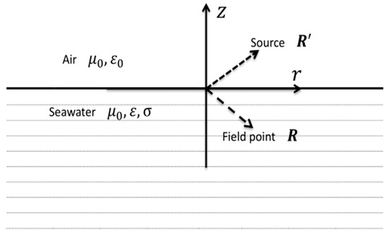
Figure 1. Air-seawater two-layer model in the cylindrical coordinate system.

The propagation constants in the two parts of the medium are

$$k_1=\omega \sqrt{{\mu }_0{\epsilon }_0}, k_2=\omega \sqrt{{\mu }_0\epsilon \left(1+\frac{\mathrm{i}\sigma }{\omega \epsilon }\right)},$$

where $\sigma$ represents magnetic conductivity tensor. ${\epsilon }_0,{\mu }_0$ are the permittivity and permeability, respectively.

Let ${\mathit{J}}_1\left({\mathit{R}}^{’}\right)$ be a current source in the air. Time harmonic factor is $e^{-i\omega t}$. ${\mathit{E}}_1\left(\mathit{R}\right)$ is the electric field in the air and ${\mathit{E}}_2\left(\mathit{R}\right)$ is the electric field in the seawater. We can obtain the wave equations as follows

$$\nabla \times \nabla \times {\mathit{E}}_1\left(\mathit{R}\right)-k_1^2{\mathit{E}}_1\left(\mathit{R}\right)=\mathrm{i}\omega {\mu }_0{\mathit{J}}_1\left({\mathit{R}}^{’}\right)z>0,$$

(38)

$$\nabla \times \nabla \times {\mathit{E}}_2\left(\mathit{R}\right)-k_2^2{\mathit{E}}_2\left(\mathit{R}\right)=0 z<0,$$

(39)

with ${\mathit{E}}_1$ and ${\mathit{E}}_2$ being subject to the following boundary and radiation conditions

$$\begin{array}{l}\widehat{n}\times \left({\mathit{E}}_1\left(\mathit{R}\right)-{\mathit{E}}_2\left(\mathit{R}\right)\right)=0 z=0,\\ \underset{r\to \infty }{\lim }r\left[\nabla \times \mathit{E}\left(\mathit{R}\right)-\mathrm{i}kr\times \mathit{E}\left(\mathit{R}\right)\right]=0.\end{array}$$

(40)

The corresponding electric DGF wave equations and boundary conditions are as follows

$$\{\begin{array}{cc}\nabla \times \nabla \times {\overline{\overline{G}}}_e^{\left(21\right)}\left(\mathit{R},{\mathit{R}}^{’}\right)-k_1^2{\overline{\overline{G}}}_e^{\left(21\right)}\left(\mathit{R},{\mathit{R}}^{’}\right)=0\hfill & \hfill z>0,\\ \nabla \times \nabla \times {\overline{\overline{G}}}_e^{\left(11\right)}\left(\mathit{R},{\mathit{R}}^{’}\right)-k_2^2{\overline{\overline{G}}}_e^{\left(11\right)}\left(\mathit{R},{\mathit{R}}^{’}\right)=\overline{\overline{I}}\delta \left(\mathit{R}-{\mathit{R}}^{’}\right)\hfill & \hfill z<0,\\ \widehat{z}\times \left({\overline{\overline{G}}}_e^{\left(11\right)}\left(\mathit{R},{\mathit{R}}^{’}\right)-{\overline{\overline{G}}}_e^{\left(21\right)}\left(\mathit{R},{\mathit{R}}^{’}\right)\right)=0\hfill & \hfill z=0,\\ \widehat{z}\times \left(\nabla \times {\overline{\overline{G}}}_e^{\left(11\right)}\left(\mathit{R},{\mathit{R}}^{’}\right)-\nabla \times {\overline{\overline{G}}}_e^{\left(21\right)}\left(\mathit{R},{\mathit{R}}^{’}\right)\right)=0\hfill & \hfill z=0,\\ \underset{r\to \infty }{\lim }r\left(\nabla \times {\overline{\overline{G}}}_e\left(\mathit{R},{\mathit{R}}^{’}\right)-\mathrm{i}kr\times {\overline{\overline{G}}}_e\left(\mathit{R},{\mathit{R}}^{’}\right)\right)=0 ,\hfill & \end{array}$$

(41)

where ${\overline{\overline{G}}}_e^{\left(11\right)}$ indicates that the field point and the source point are both in the seawater, ${\overline{\overline{G}}}_e^{\left(21\right)}$ denotes that the field point is in the seawater and the source point is in the air. The relations between the electric DGF and the electric field are

$$\begin{array}{l}{\mathit{E}}_1\left(\mathit{R}\right)=\mathrm{i}\omega {\mu }_0{\displaystyle {\iiint }_{V_2}{\overline{\overline{G}}}_e^{\left(11\right)}\left(\mathit{R},{\mathit{R}}^{’}\right)\cdot {\mathit{J}}_1\left({\mathit{R}}^{’}\right)d{V}^{’}},\\ {\mathit{E}}_2\left(\mathit{R}\right)=\mathrm{i}\omega {\mu }_0{\displaystyle {\iiint }_{V_2}{\overline{\overline{G}}}_e^{\left(21\right)}\left(\mathit{R},{\mathit{R}}^{’}\right)\cdot {\mathit{J}}_1\left({\mathit{R}}^{’}\right)d{V}^{’}.}\end{array}$$

(42)

It is, easy to show that once we know ${\overline{\overline{G}}}_e^{\left(11\right)}$ and ${\overline{\overline{G}}}_e^{\left(21\right)}$, ${\mathit{E}}_1\left(\mathit{R}\right)$ and ${\mathit{E}}_2\left(\mathit{R}\right)$ can be obtained. To begin with, we should introduce the electric DGF, and then, we can get the electric field.

Theorem 3.

Assume that $\mathit{M}$ and $\mathit{N}$ are the vector wave functions of $\mathit{R}$, ${\mathit{M}}^{’}$ and ${\mathit{N}}^{’}$ are the vector wave functions of ${\mathit{R}}^{’}$. $\lambda$ and $h$ are continuous eigenvalues. The electric DGF in the cylindrical coordinate system can be written as

$${\overline{\overline{G}}}_{e0}(\mathit{R},{\mathit{R}}^{’}) =\{\begin{array}{l}-\frac{1}{k^2}\widehat{z}\widehat{z}\delta (\mathit{R}-{\mathit{R}}^{’})+{\displaystyle {\int }_0^{\infty }d\lambda }{\displaystyle \sum _{n=0}^{\infty }C[\mathit{M}(h){\mathit{M}}^{’}(-h) (z>z^{’})}\\ +\mathit{N}(h){\mathit{N}}^{’}(-h)]\\ -\frac{1}{k^2}\widehat{z}\widehat{z}\delta (\mathit{R}-{\mathit{R}}^{’})+{\displaystyle {\int }_0^{\infty }d\lambda }{\displaystyle \sum _{n=0}^{\infty }C[\mathit{M}(-h){\mathit{M}}^{’}(h) (z<z^{’})}\\ +\mathit{N}(-h){\mathit{N}}^{’}(h)]\end{array},$$

(43)

where

$$C=\frac{2-{\delta }_0}{4\pi \lambda h_2}, h=\sqrt{k^2-{\lambda }^2}.$$

${\delta }_0$is defined as follows

$${\delta }_0=\{\begin{array}{l}1 n=0 \\ 0 n\ne 0\end{array}.$$

where $n$ identifies the eigenvalue parameter.

Proof. 

The cylindrical vector wave functions $\mathit{M}$ and $\mathit{N}$ can be defined by

$${\mathit{M}}_{en\lambda }(h)=\left[-\frac{n{J}_n(\lambda r)}{r}\sin (n\phi )\widehat{r}-\frac{\partial J_n(\lambda r)}{\partial r}\cos (n\phi )\widehat{\phi }\right]e^{\mathrm{i}hz},$$

(44)

$${\mathit{M}}_{on\lambda }(h)=\left[\frac{n{J}_n(\lambda r)}{r}\cos (n\phi )\widehat{r}-\frac{\partial J_n(\lambda r)}{\partial r}\sin (n\phi )\widehat{\phi }\right]e^{\mathrm{i}hz},$$

(45)

$$\begin{array}{l}{\mathit{N}}_{en\lambda }(h)=\frac{1}{\kappa }[\mathrm{i}h\frac{\partial J_n(\lambda r)}{\partial r}\cos (n\phi )\widehat{r}-\frac{\mathrm{i}hn}{r}{J}_n(\lambda r)\sin (n\phi )\widehat{\phi }\\ +{\lambda }^2{J}_n(\lambda r)\cos (n\phi )\widehat{z}]e^{\mathrm{i}hz},\end{array}$$

(46)

$$\begin{array}{l}{\mathit{N}}_{on\lambda }(h)=\frac{1}{\kappa }[\mathrm{i}h\frac{\partial J_n(\lambda r)}{\partial r}\sin (n\phi )\widehat{r}+\frac{\mathrm{i}hn}{r}{J}_n(\lambda r)\cos (n\phi )\widehat{\phi }\\ +{\lambda }^2{J}_n(\lambda r)\sin (n\phi )\widehat{z}]e^{\mathrm{i}hz},\end{array}$$

(47)

where ${\kappa }^2=h^2+{\lambda }^2$.$J_n(\lambda r)$ represents the n-order Bessel function. $o$ and $e$ denote the odd and the even function, respectively. The functions $\mathit{M}(h)$ describe the electric field of $T{E}_{mn}$ mode in a cylindrical waveguide and the functions $\mathit{N}(h)$ for the $T{M}_{mn}$ mode. The cylindrical vector wave functions are defined in the range of $0\le r<\infty$, $0\le \phi <2\pi$, $-\infty \le z<\infty$.

The trick of the proof is to find the magnetic DGF of free space ${\overline{\overline{G}}}_{m1}(\mathit{R},{\mathit{R}}^{’})$, which satisfies

$$\nabla \times \nabla \times {\overline{\overline{G}}}_{m1}(\mathit{R},{\mathit{R}}^{’})-k^2{\overline{\overline{G}}}_{m1}(\mathit{R},{\mathit{R}}^{’})=\nabla \times \overline{\overline{I}}\delta (\mathit{R}-{\mathit{R}}^{’}) ,$$

(48)

where $\overline{\overline{I}}\delta (\mathit{R}-{\mathit{R}}^{’})$ is the source function and $k$ represents the wave number.

For cylindrical vector wave functions involving continuous eigenvalues, we assume that the source function is given by

$$\nabla \times \left[\overline{\overline{I}}\delta (\mathit{R}-\mathit{R}’)\right]={\displaystyle {\int }_0^{\infty }d\lambda {\displaystyle {\int }_{-\infty }^{\infty }dh}{\displaystyle \sum _{\mathit{N}=0}^{\infty }\left[\mathit{N}(h)A(h)+\mathit{M}(h)B(h)\right]}},$$

(49)

where $A(h)$ and $B(h)$ are two undetermined position vector coefficients. $\lambda$ and $h$ are continuous eigenvalues. Due to the linear correlation between $J_n(\lambda r)$ and $J_n(-\lambda r)$, the integral range of $\lambda$ is $(0,+\infty )$. After taking the dot product of (46) with ${\mathit{N}}_{e{m}^{’}{n}^{’}}(-h^{’})$ and integrating over volume $V$, we have

$$\begin{array}{ll}& {\displaystyle {\iiint }_V\mathit{N}(-h^{’})\cdot \nabla \times \left[\overline{\overline{I}}\delta (\mathit{R}-\mathit{R}’)\right]dV}\\ =& {\displaystyle {\iiint }_{V}dV}{\displaystyle {\int }_0^{+\infty }d\lambda {\displaystyle {\int }_{-\infty }^{\infty }dh}{\displaystyle \sum _{n=0}^{\infty }\mathit{N}(-h^{’})\cdot \left[\mathit{N}(h)A(h)+\mathit{M}(h)B(h)\right]}.}\end{array}$$

(50)

Using the orthogonality of the vector wave functions and the normalization coefficient formula, we get

$$A\left(h\right)=\frac{(2-{\delta }_0)\kappa }{4{\pi }^2\lambda }{\mathit{M}}^{’}(-h).$$

(51)

Similarly, we can obtain

$$B\left(h\right)=\frac{(2-{\delta }_0)\kappa }{4{\pi }^2\lambda }{\mathit{N}}^{’}(-h),$$

(52)

where

$$\kappa =\sqrt{{\lambda }^2+h^2},$$

and ${\delta }_0$ is defined as the Kronecker delta function respect to $n$

$${\delta }_0=\{\begin{array}{l}1 n=0 \\ 0 n\ne 0\end{array}.$$

Thus, we can get the eigenfunction expansion of the source function as follows

$$\begin{array}{ll}\nabla \times [\overline{\overline{I}}\delta (\mathit{R}-{\mathit{R}}^{’})]=& {\displaystyle {\int }_0^{\infty }d\lambda }{\displaystyle {\int }_{-\infty }^{\infty }dh{\displaystyle \sum _{n=0}^{\infty }\frac{(2-{\delta }_0)\kappa }{4{\pi }^2\lambda } }}\\ & \cdot \left[\mathit{N}(h){\mathit{M}}^{’}(-h)+\mathit{M}(h){\mathit{N}}^{’}(-h)\right].\end{array}$$

(53)

Substituting (53) into (48), ${\overline{\overline{G}}}_{m1}(\mathit{R},{\mathit{R}}^{’})$ can be computed by

$$\begin{array}{ll}{\overline{\overline{G}}}_{m1}(\mathit{R},{\mathit{R}}^{’})=& {\displaystyle {\int }_0^{\infty }d\lambda }{\displaystyle {\int }_{-\infty }^{\infty }dh{\displaystyle \sum _{n=0}^{\infty }\frac{(2-{\delta }_0)\kappa }{4{\pi }^2\lambda ({\kappa }^2-k^2)}}}\\ & \cdot \left[\mathit{N}(h){\mathit{M}}^{’}(-h)+\mathit{M}(h){\mathit{N}}^{’}(-h)\right].\end{array}$$

(54)

Because the pole of the integral is located in $h=\pm h_1,h_1=\sqrt{k_1{}^2-{\lambda }^2}$, the ${\overline{\overline{G}}}_{m1}(\mathit{R},{\mathit{R}}^{’})$ can be obtained from the residue theory

$${\overline{\overline{G}}}_{m1}(\mathit{R},{\mathit{R}}^{’})=\{\begin{array}{l}k{\displaystyle {\int }_0^{\infty }d\lambda }{\displaystyle \sum _{n=0}^{\infty }C\cdot \left[\mathit{N}(h){\mathit{M}}^{’}(-h)+\mathit{M}(h){\mathit{N}}^{’}(-h) \right] (z>z^{’})},\\ k{\displaystyle {\int }_0^{\infty }d\lambda }{\displaystyle \sum _{n=0}^{\infty }C\cdot \left[\mathit{N}(-h){\mathit{M}}^{’}(h)+\mathit{M}(-h){\mathit{N}}^{’}(h)\right] (z<z^{’}),}\end{array}$$

(55)

where

$$C=\frac{2-{\delta }_0}{4\pi \lambda h_1}.$$

Due to the relation of electric DGF and magnetic DGF

$$\nabla \times {\overline{\overline{G}}}_{m1}(\mathit{R},{\mathit{R}}^{’})=\overline{\overline{I}}\delta (\mathit{R}-{\mathit{R}}^{’})+k^2{\overline{\overline{G}}}_{e1}(\mathit{R},{\mathit{R}}^{’}) ,$$

(56)

we can get the electric DGF ${\overline{\overline{G}}}_{e1}$ in the cylindrical coordinate system

$${\overline{\overline{G}}}_{e1}(\mathit{R},{\mathit{R}}^{’}) =\{\begin{array}{l}-\frac{1}{k^2}\widehat{z}\widehat{z}\delta (\mathit{R}-{\mathit{R}}^{’})+{\displaystyle {\int }_0^{\infty }d\lambda }{\displaystyle \sum _{n=0}^{\infty }C[\mathit{M}(h){\mathit{M}}^{’}(-h) (z>z^{’})}\\ +\mathit{N}(h){\mathit{N}}^{’}(-h)] \\ -\frac{1}{k^2}\widehat{z}\widehat{z}\delta (\mathit{R}-{\mathit{R}}^{’})+{\displaystyle {\int }_0^{\infty }d\lambda }{\displaystyle \sum _{n=0}^{\infty }C[\mathit{M}(-h){\mathit{M}}^{’}(h) (z<z^{’})}\\ +\mathit{N}(-h){\mathit{N}}^{’}(h)] \end{array},$$

(57)

where ${\mathit{M}}^{’}$ and ${\mathit{N}}^{’}$ are the vector wave functions of ${\mathit{R}}^{’}$. The proof is completed. □

Next, we discuss the DGF of the two-layer model. It is observed from Figure 1 that when the source is in the air, the electric field in the air comes from the superposition of the scattering field of the source point and the field point. The electric field in the seawater is equal to the scattering field in the seawater. From the above analysis, the DGF for two-layer model is therefore given by

$$\begin{array}{l}{\overline{\overline{G}}}_e^{\left(11\right)}={\overline{\overline{G}}}_{e1}^{\left(1\right)}+{\overline{\overline{G}}}_{es}^{\left(11\right)},\\ {\overline{\overline{G}}}_e^{\left(21\right)}={\overline{\overline{G}}}_{es}^{\left(21\right)}.\end{array}$$

(58)

What we discussed above is called the principle of scattering superposition, which is widely applied to solve multilayer medium model.

Suppose that

$$\begin{array}{l}{\overline{\overline{G}}}_{es}^{\left(11\right)}(\mathit{R},{\mathit{R}}^{’})={\displaystyle {\int }_0^{\infty }d\lambda }{\displaystyle \sum _{n}C\left[a\mathit{M}\left(h_1\right){\mathit{M}}^{’}\left(h_1\right)+b\mathit{N}\left(h_1\right){\mathit{N}}^{’}\left(h_1\right)\right]} ,\\ {\overline{\overline{G}}}_{es}^{\left(21\right)}(\mathit{R},{\mathit{R}}^{’})={\displaystyle {\int }_0^{\infty }d\lambda }{\displaystyle \sum _{n}C\left[c\mathit{M}\left(-h_2\right){\mathit{M}}^{’}\left(h_1\right)+d\mathit{N}\left(-h_2\right){\mathit{N}}^{’}\left(h_1\right)\right]} ,\end{array}$$

(59)

where $h_1=\sqrt{k_1{}^2-k_c{}^2}$, $h_2=\sqrt{k_2{}^2-k_c{}^2}$. $\mathit{M}\left(h_1\right)$ and $\mathit{N}\left(h_1\right)$ are vector wave functions in the air. $\mathit{M}\left(-h_2\right)$ and $\mathit{N}\left(-h_2\right)$ are the solutions of the wave equations in seawater. $a,b,c,d$ are the unknown coefficients. To determine the unknown coefficients in the assumed DGFs, the boundary conditions (41) have to be satisfied at $z=0$. Combined with the principle of scattering superposition (58), we find

$$\begin{array}{l}a=\frac{h_1-h_2}{h_1+h_2}, b=\frac{{\eta }^2{h}_1-h_2}{{\eta }^2{h}_1+h_2},\\ c=\frac{2h_1}{h_1+h_2}, d=\frac{2\eta h_1}{{\eta }^2{h}_1+h_2},\end{array}$$

(60)

where $\eta =\frac{k_2}{k_1}$.

In summary, when the source is in air, the electric DGF of two-layer medium model can be expressed as

$$\begin{array}{c}\hfill {\overline{\overline{G}}}_e{}^{(11)}(\mathit{R},{\mathit{R}}^{’})=-\frac{1}{k^2}\widehat{z}\widehat{z}\delta (\mathit{R}-{\mathit{R}}^{’})+{\displaystyle {\int }_0^{\infty }d\lambda }{\displaystyle \sum _{n=0}^{\infty }C\{\mathit{M}(h_1)\left[{\mathit{M}}^{’}(-h_1)+a{\mathit{M}}^{’}(h_1)\right]}\\ \hfill +\mathit{N}(h_1)\left[{\mathit{N}}^{’}(-h_1)+b{\mathit{N}}^{’}(h_1)\right]\} ,\end{array}$$

(61)

$${\overline{\overline{G}}}_e^{\left(21\right)}(\mathit{R},{\mathit{R}}^{’})={\displaystyle {\int }_0^{\infty }d\lambda }{\displaystyle \sum _{n=0}^{\infty }C\left[c\mathit{M}\left(-h_2\right){\mathit{M}}^{’}\left(h_1\right)+d\mathit{N}\left(-h_2\right){\mathit{N}}^{’}\left(h_1\right)\right]} ,$$

(62)

where ${\overline{\overline{G}}}_e{}^{(11)}(\mathit{R},{\mathit{R}}^{’})$ indicates the DGF of the upper level, and ${\overline{\overline{G}}}_e{}^{(21)}(\mathit{R},{\mathit{R}}^{’})$ represents the DGF of the lower level.

According to the DGF of two-layer model, the electric field in air and seawater can be calculated by

$${\mathit{E}}_1(\mathit{R})=\mathrm{i}\omega {\mu }_0{\displaystyle {\iiint }_V{\overline{\overline{G}}}_e^{\left(11\right)}(\mathit{R},{\mathit{R}}^{’})\cdot {\mathit{J}}_1({\mathit{R}}^{’})d{V}^{’}},$$

(63)

$${\mathit{E}}_2(\mathit{R})=\mathrm{i}\omega {\mu }_0{\displaystyle {\iiint }_V{\overline{\overline{G}}}_e^{\left(21\right)}(\mathit{R},{\mathit{R}}^{’})\cdot {\mathit{J}}_1({\mathit{R}}^{’})d{V}^{’}},$$

(64)

where ${\mathit{J}}_1({\mathit{R}}^{’})$ denotes the current source in the air.

Suppose that there is an infinitely small vertical electric dipole in the air whose coordinate is ${\mathit{R}}^{’}{=(0,0,\mathrm{z}}_0)$. $c\widehat{z}$ indicates the current moment. The current density of an electric dipole in the air can be expressed as

$${\mathit{J}}_1({\mathit{R}}^{’})=c\widehat{z}\delta (x^{’})\delta (y^{’})\delta (z^{’}-z_0),$$

(65)

where

$$c=\frac{4\pi k_1{}^2}{\mathrm{i}\omega {\mu }_0}.$$

By substituting ${\mathit{R}}^{’}{=(0,0,\mathrm{z}}_0)$ into the vector wave functions (41)~(44), vector wave functions are simplified to

$${\mathit{M}}^{’}{}_{en\lambda }(h)=0,$$

(66)

$${\mathit{M}}^{’}{}_{on\lambda }(h)=0,$$

(67)

$${\mathit{N}}^{’}{}_{en\lambda }(h)=\frac{1}{\kappa }\left[{\lambda }^2{J}_n(\lambda r)\cos (n\phi )\widehat{z}\right]e^{\mathrm{i}hz},$$

(68)

$${\mathit{N}}^{’}{}_{on\lambda }(h)=\frac{1}{\kappa }\left[{\lambda }^2{J}_n(\lambda r)\sin (n\phi )\widehat{z}\right]e^{\mathrm{i}hz}.$$

(69)

As we can see, the vector wave functions are more concise in form than before. If we plug simplified vector wave functions back into (61) and (62), we have

$${\overline{\overline{G}}}_e{}^{(11)}(\mathit{R},{\mathit{R}}^{’})=\frac{\mathrm{i}(2-{\delta }_0)}{4\pi \kappa }{\displaystyle {\int }_0^{\infty }\left(\frac{\lambda }{h_1}\right)}{J}_0(\lambda r){\mathit{N}}_{e0\lambda }\left(h_1\right)\left(e^{-\mathrm{i}{h}_1{z}_0}+b{e}^{\mathrm{i}{h}_1{z}_0}\right)d\lambda ,$$

(70)

$${\overline{\overline{G}}}_e{}^{(21)}(\mathit{R},{\mathit{R}}^{’})=\frac{\mathrm{i}(2-{\delta }_0)}{4\pi \kappa }{\displaystyle {\int }_0^{\infty }\left(\frac{\lambda }{h_2}\right)}{J}_0(\lambda r){\mathit{N}}_{e0\lambda }\left(-h_2\right)d{e}^{\mathrm{i}{h}_1{z}_0}d\lambda .$$

(71)

Once we have the DGF, the electric field can be solved immediately. By applying (63) and (64), the electric field in the air and seawater can be expressed in the form of

$${\mathit{E}}_1(\mathit{R})=\mathrm{i}{k}_1{\displaystyle {\int }_0^{\infty }\left(\frac{\lambda }{h_1}\right)}{J}_0(\lambda r){\mathit{N}}_{e0\lambda }\left(h_1\right)\left(e^{-\mathrm{i}{h}_1{z}_0}+b{e}^{\mathrm{i}{h}_1{z}_0}\right)d\lambda ,$$

(72)

$${\mathit{E}}_2(\mathit{R})=\mathrm{i}{k}_1{\displaystyle {\int }_0^{\infty }\left(\frac{\lambda }{h_2}\right)}{J}_0(\lambda r){\mathit{N}}_{e0\lambda }\left(-h_2\right)d{e}^{\mathrm{i}{h}_1{z}_0}d\lambda .$$

(73)

The Bessel function in the above electric field expression is obviously not conducive to the solution of the electric field. It is worth noting that the Bessel function can be expressed by asymptotic expression when $\lambda r$ is large enough; the vector wave functions, therefore, become

$${\mathit{M}}_{en\lambda }\left(h\right)\simeq {\left(-\mathrm{i}\right)}^{n+\frac{3}{2}}\lambda {\left(\frac{2}{\pi \lambda r}\right)}^2{e}^{\mathrm{i}\lambda r+hz}\cos n\varphi \widehat{\varphi },$$

(74)

$${\mathit{M}}_{on\lambda }\left(h\right)\simeq {\left(-\mathrm{i}\right)}^{n+\frac{3}{2}}\lambda {\left(\frac{2}{\pi \lambda r}\right)}^2{e}^{\mathrm{i}\lambda r+hz}\sin n\varphi \widehat{\varphi },$$

(75)

$${\mathit{N}}_{en\lambda }\left(h\right)\simeq {\left(-\mathrm{i}\right)}^{n+\frac{1}{2}}\frac{\lambda }{k_0}{\left(\frac{2}{\pi \lambda r}\right)}^2{e}^{\mathrm{i}\lambda r+hz}\cos n\varphi \left(-h\widehat{r}+\lambda \widehat{z}\right),$$

(76)

$${\mathit{N}}_{on\lambda }\left(h\right)\simeq {\left(-\mathrm{i}\right)}^{n+\frac{1}{2}}\frac{\lambda }{k_0}{\left(\frac{2}{\pi \lambda r}\right)}^2{e}^{\mathrm{i}\lambda r+hz}\sin n\varphi \left(-h\widehat{r}+\lambda \widehat{z}\right).$$

(77)

The approximate expressions for electric field, using (46) with the functions ${\mathit{N}}_{en\lambda }\left(-h_2\right)$ and ${\mathit{N}}_{en\lambda }\left(h_1\right)$ replaced by above equations, can be solved efficiently and easily.

For the two-layer model in cylindrical coordinate system, the approximation of the electric field has been obtained by using the asymptotic expression of the far-zone field. Compared with the integral of Bessel function, the simplified electric field can handle the mathematical difficulties.

4.2. The Two-Layer Model in the Space Rectangular Coordinate System

We now turn to the two-layer model in space rectangular coordinate system. It is apparent from Figure 2 that the sea level $z=0$ divides the air and seawater into two parts.

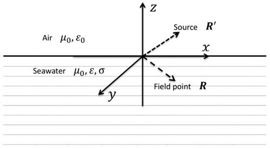
Figure 2. Air-Seawater two-layer model in space rectangular coordinate system.

Similarly, electric DGF also satisfies the wave equations and boundary conditions (41). Next, we need to introduce the following vector wave functions of rectangular coordinate system. The vector wave functions $\mathit{M}$ and $\mathit{N}$ are defined as

$${\mathit{M}}_{emn}\left(h\right)=\left(-\frac{n\pi }{b}\cos \frac{m\pi x}{a}\sin \frac{n\pi y}{b}\widehat{x}+\frac{m\pi }{a}\sin \frac{m\pi x}{a}\cos \frac{n\pi y}{b}\widehat{y}\right)e^{\mathrm{i}hz},$$

(78)

$${\mathit{M}}_{omn}\left(h\right)=\left(\frac{n\pi }{b}\sin \frac{m\pi x}{a}\cos \frac{n\pi y}{b}\widehat{x}-\frac{m\pi }{a}\cos \frac{m\pi x}{a}\sin \frac{n\pi y}{b}\widehat{y}\right)e^{\mathrm{i}hz},$$

(79)

$$\begin{array}{l}{\mathit{N}}_{omn}\left(h\right)=\frac{1}{\kappa }[\mathrm{i}h\frac{m\pi }{a}\cos \frac{m\pi x}{a}\sin \frac{n\pi y}{b}\widehat{x}+ih\frac{n\pi }{b}\sin \frac{m\pi x}{a}\cos \frac{n\pi y}{b}\widehat{y}\\ +\left(\frac{m^2{\pi }^2}{a^2}+\frac{n^2{\pi }^2}{b^2}\right)\sin \frac{m\pi x}{a}\sin \frac{n\pi y}{b}\widehat{z}]e^{\mathrm{i}hz},\end{array}$$

(80)

$$\begin{array}{l}{\mathit{N}}_{emn}\left(h\right)=\frac{1}{\kappa }[-\mathrm{i}h\frac{m\pi }{a}\sin \frac{m\pi x}{a}\cos \frac{n\pi y}{b}\widehat{x}-ih\frac{n\pi }{b}\cos \frac{m\pi x}{a}\sin \frac{n\pi y}{b}\widehat{y}\\ +\left(\frac{m^2{\pi }^2}{a^2}+\frac{n^2{\pi }^2}{b^2}\right)\cos \frac{m\pi x}{a}\cos \frac{n\pi y}{b}\widehat{z}]e^{\mathrm{i}hz},\end{array}$$

(81)

where $o$ and $e$ stand for the odd and the even functions, respectively. $m$ and $n$ stand for the eigenvalue parameters. It can be easily shown that the magnetic DGF ${\overline{\overline{G}}}_{m2}(\mathit{R},{\mathit{R}}^{’})$ satisfies

$$\nabla \times \nabla \times {\overline{\overline{G}}}_{m2}(\mathit{R},{\mathit{R}}^{’})-k^2{\overline{\overline{G}}}_{m2}(\mathit{R},{\mathit{R}}^{’})=\nabla \times \overline{\overline{I}}\delta (\mathit{R}-{\mathit{R}}^{’}) .$$

(82)

The domain is $0\le x\le a$, $0\le y\le b$, $-\infty \le z\le +\infty$. When $x=0,x=a$ and $y=0,y=b$, the boundary condition is

$$\widehat{n}\times \nabla \times {\overline{\overline{G}}}_{m2}(\mathit{R},{\mathit{R}}^{’})=0 .$$

(83)

Since ${\mathit{N}}_{emn}(h)$ and ${\mathit{M}}_{omn}(h)$ satisfy the boundary condition defined by (79), we assume that the eigenfunction expression of the source function is

$$\nabla \times \left[\overline{\overline{I}}\delta (\mathit{R}-\mathit{R}’)\right]={\displaystyle {\int }_{-\infty }^{+\infty }dh{\displaystyle \sum _{m,n}\left[{\mathit{N}}_{emn}(h)A_{emn}(h)+{\mathit{M}}_{omn}(h)B_{omn}(h)\right]}},$$

(84)

where $A_{emn}(h)$ and $B_{omn}(h)$ are two undetermined position vector coefficients. In order to solve these two coefficients, we need to take the dot product of (80) with ${\mathit{N}}_{e{m}^{’}{n}^{’}}(-h^{’})$ and integrate over volume $V$

$$\begin{array}{ll}& {\displaystyle {\iiint }_V{\mathit{N}}_{e{m}^{’}{n}^{’}}(-h^{’})\cdot \nabla \times \left[\overline{\overline{I}}\delta (\mathit{R}-\mathit{R}’)\right]dV}\\ =& {\displaystyle {\iiint }_{V}dV}{\displaystyle {\int }_{-\infty }^{+\infty }dh{\displaystyle \sum _{m,n}{\mathit{N}}_{e{m}^{’}{n}^{’}}(-h^{’})\cdot \left[{\mathit{N}}_{emn}(h)A_{emn}(h)+{\mathit{M}}_{omn}(h)B_{omn}(h)\right]}} .\end{array}$$

(85)

Applying the dyadic calculation formula $\nabla \times \nabla \times \overline{\overline{A}}=\nabla (\nabla \cdot \overline{\overline{A}})-\nabla \cdot (\nabla \overline{\overline{A}})$ to the left-hand side of (81) yields

$${\displaystyle {\iiint }_V\nabla \times {\mathit{N}}_{e{m}^{’}{n}^{’}}(-h^{’})\cdot \overline{\overline{I}}\delta (\mathit{R}-{\mathit{R}}^{’})-\nabla \cdot {\mathit{N}}_{e{m}^{’}{n}^{’}}(-h^{’})\times \overline{\overline{I}}\delta (\mathit{R}-{\mathit{R}}^{’})dV}.$$

(86)

By the Dyadic Gauss theorem, we have

$${\nabla }^{’}{\mathit{N}}^{’}{}_{e{m}^{’}{n}^{’}}(-h^{’})-{\displaystyle {∯}_S\widehat{n}\cdot \left[{\mathit{N}}_{e{m}^{’}{n}^{’}}(-h^{’})\times \overline{\overline{I}}\delta (\mathit{R}-{\mathit{R}}^{’})\right]}dS,$$

(87)

where ${\nabla }^{’}$ is used to indicate the gradient operator on the variable $\left(x^{’},y^{’},z^{’}\right)$. Since $R^{’}$ is in $V$, the surface integral in (83) is equal to zero. Using the orthogonality of the vector wave functions and the normalization coefficient formula, we can rewrite the right-hand side of (81) as

$$\left(1+{\delta }_0\right)\frac{\pi ab}{2}\left[{\left(\frac{m^{’}\pi }{a}\right)}^2+{\left(\frac{n^{’}\pi }{b}\right)}^2\right]A_{e{m}^{’}{n}^{’}}\left(h^{’}\right).$$

(88)

In conclusion, (81) can be rewritten as

$${\nabla }^{’}{\mathit{N}}^{’}{}_{e{m}^{’}{n}^{’}}(-h^{’})=\left(1+{\delta }_0\right)\frac{\pi ab}{2}{k}_c^{’}{}^2{A}_{e{m}^{’}{n}^{’}}\left(h^{’}\right).$$

(89)

Thus, $A_{emn}\left(h^{’}\right)$ is given by

$$A_{emn}\left(h\right)=\frac{(2-{\delta }_0)\kappa }{\pi ab{k}_c{}^2}{\mathit{M}}^{’}{}_{emn}(-h).$$

(90)

Similarly, we obtain

$$B_{omn}\left(h\right)=\frac{(2-{\delta }_0)\kappa }{\pi ab{k}_c{}^2}{\mathit{N}}^{’}{}_{omn}(-h),$$

(91)

where

$$\begin{array}{l}\kappa =\sqrt{k_c{}^2+h^2},\\ k_c{}^2={\left(\frac{m\pi }{a}\right)}^2+{\left(\frac{n\pi }{b}\right)}^2.\end{array}$$

Therefore, we can get the eigenfunction expression of the source function as follows

$$\begin{array}{l}\nabla \times [\overline{\overline{I}}\delta (\mathit{R}-{\mathit{R}}^{’})]={\displaystyle {\int }_{-\infty }^{+\infty }dh{\displaystyle \sum _{m,n}\frac{(2-{\delta }_0)\kappa }{\pi ab{k}_c{}^2}}}\\ \cdot \left[{\mathit{N}}_{emn}(h){\mathit{M}}^{’}{}_{emn}(-h)+{\mathit{M}}_{omn}(h){\mathit{N}}^{’}{}_{omn}(-h)\right].\end{array}$$

(92)

Inserting the expression (88) into (78) gives

$$\begin{array}{ll}{\overline{\overline{G}}}_{m2}(\mathit{R},{\mathit{R}}^{’})=& {\displaystyle {\int }_{-\infty }^{+\infty }dh{\displaystyle \sum _{m,n}\frac{(2-{\delta }_0)\kappa }{\pi ab({\kappa }^2-k^2)}}}\\ & \cdot \left[{\mathit{N}}_{emn}(h){\mathit{M}}^{’}{}_{emn}(-h)+{\mathit{M}}_{omn}(h)\mathit{N}{’}_{omn}(-h)\right].\end{array}$$

(93)

Using the loop integral method, the Fourier integral in (89) can be obtained. Since ${\kappa }^2-k^2=k_c{}^2+h^2-k^2$, the integral has two poles at $h=\pm \sqrt{k^2-k_c{}^2}$, and satisfies Jordan lemma at infinity. Furthermore, (89) can be derived as

$${\overline{\overline{G}}}_{m2}(\mathit{R},{\mathit{R}}^{’})=\{\begin{array}{l}{\displaystyle \sum _{m,n}kC\cdot \left[{\mathit{N}}_{emn}(h){\mathit{M}}^{’}{}_{emn}(-h)+{\mathit{M}}_{omn}(h){\mathit{N}}^{’}{}_{omn}(-h)\right] (z>z^{’})} \\ {\displaystyle \sum _{m,n}kC\cdot \left[{\mathit{N}}_{emn}(-h){\mathit{M}}^{’}{}_{emn}(h)+{\mathit{M}}_{omn}(-h){\mathit{N}}^{’}{}_{omn}(h)\right] (z<z^{’})}\end{array},$$

(94)

where

$$C=\frac{(2-{\delta }_0)\mathrm{i}}{ab{k}_c{}^{2}h}.$$

where ${\mathit{M}}^{’}$ and ${\mathit{N}}^{’}$ are the vector wave functions of ${\mathit{R}}^{’}$. $\delta$ is defined as.

$$\delta =\{\begin{array}{l}1 \mathrm{for} n=0 or m=0\\ 0 \mathrm{else}\end{array}.$$

(95)

Suppose that the source is in the air, using the scattering field superposition method, we have

$$\begin{array}{l}{\overline{\overline{G}}}_e^{\left(11\right)}={\overline{\overline{G}}}_{e2}^{\left(1\right)}+{\overline{\overline{G}}}_{es}^{\left(11\right)},\\ {\overline{\overline{G}}}_e^{\left(21\right)}={\overline{\overline{G}}}_{es}^{\left(21\right)},\end{array}$$

(96)

where ${\overline{\overline{G}}}_e{}^{(11)}(\mathit{R},{\mathit{R}}^{’})$ is the DGF in the air, ${\overline{\overline{G}}}_e{}^{(21)}(\mathit{R},{\mathit{R}}^{’})$ represents the DGF in the seawater.

Assume that ${\overline{\overline{G}}}_{es}^{\left(11\right)}(\mathit{R},{\mathit{R}}^{’})$ and ${\overline{\overline{G}}}_{es}^{\left(21\right)}(\mathit{R},{\mathit{R}}^{’})$ are

$$\begin{array}{l}{\overline{\overline{G}}}_{es}^{\left(11\right)}(\mathit{R},{\mathit{R}}^{’})={\displaystyle \sum _{m,n}C\left[a_1\mathit{M}\left(h_1\right){\mathit{M}}^{’}\left(h_1\right)+b_1\mathit{N}\left(h_1\right){\mathit{N}}^{’}\left(h_1\right)\right]} ,\\ {\overline{\overline{G}}}_{es}^{\left(21\right)}(\mathit{R},{\mathit{R}}^{’})={\displaystyle \sum _{m,n}C\left[c_1\mathit{M}\left(-h_2\right){\mathit{M}}^{’}\left(h_1\right)+d_1\mathit{N}\left(-h_2\right){\mathit{N}}^{’}\left(h_1\right)\right]},\end{array}$$

(97)

where $h_1=\sqrt{k_1{}^2-k_c{}^2}$, $h_2=\sqrt{k_2{}^2-k_c{}^2}$. $\mathit{M}\left(h_1\right)$ and $\mathit{N}\left(h_1\right)$ are the solutions of the wave equations in the air, $\mathit{M}\left(-h_2\right)$ and $\mathit{N}\left(-h_2\right)$ are the solutions of the wave equations in seawater. $a_1,b_1,c_1,d_1$ are the unknown coefficients. Combining with the boundary conditions (41), we can obtain the values of the unknown coefficients

$$\begin{array}{l}{a}_1=\frac{h_1-h_2}{h_1+h_2}, b_1=\frac{{\eta }^2{h}_1-h_2}{{\eta }^2{h}_1+h_2},\\ c_1=\frac{2h_1}{h_1+h_2}, d_1=\frac{2\eta h_1}{{\eta }^2{h}_1+h_2},\end{array}$$

(98)

where $\eta =\frac{k_2}{k_1}$.

In the space rectangular coordinate system, when the source is in air, the DGF of the two-layer medium model can be expressed as

$$\begin{array}{c}\hfill {\overline{\overline{G}}}_e{}^{(11)}(\mathit{R},{\mathit{R}}^{’})=-\frac{1}{k^2}\widehat{z}\widehat{z}\delta (\mathit{R}-{\mathit{R}}^{’})+{\displaystyle \sum _{m=0}^{\infty }{\displaystyle \sum _{n=0}^{\infty }C\{\mathit{M}(h_1)\left[{\mathit{M}}^{’}(-h_1)+a_1{\mathit{M}}^{’}(h_1)\right] }}\\ \hfill +\mathit{N}(h_1)\left[{\mathit{N}}^{’}(-h_1)+b_1{\mathit{N}}^{’}(h_1)\right]\} ,\end{array}$$

(99)

$${\overline{\overline{G}}}_e^{\left(21\right)}(\mathit{R},{\mathit{R}}^{’})={\displaystyle \sum _{m=0}^{\infty }{\displaystyle \sum _{n=0}^{\infty }C\left[c_1\mathit{M}\left(-h_2\right){\mathit{M}}^{’}\left(h_1\right)+d_1\mathit{N}\left(-h_2\right){\mathit{N}}^{’}\left(h_1\right)\right]}} .$$

(100)

It can be seen that the DGFs in the space rectangular coordinate system and the cylindrical coordinate system are very similar in form.

The electric field is calculated by DGFs. After solving the system, we can get the electric field in air and seawater

$${\mathit{E}}_1(\mathit{R})=\mathrm{i}\omega {\mu }_0{\displaystyle {\iiint }_V{\overline{\overline{G}}}_e^{\left(11\right)}(\mathit{R},{\mathit{R}}^{’})\cdot {\mathit{J}}_1({\mathit{R}}^{’})d{V}^{’}},$$

(101)

$${\mathit{E}}_2(\mathit{R})=\mathrm{i}\omega {\mu }_0{\displaystyle {\iiint }_V{\overline{\overline{G}}}_e^{\left(21\right)}(\mathit{R},{\mathit{R}}^{’})\cdot {\mathit{J}}_1({\mathit{R}}^{’})d{V}^{’}},$$

(102)

where ${\mathit{J}}_1({\mathit{R}}^{’})$ represents the current source in the air.

4.3. The Two-Layer Model in the Sphere Coordinate System

In this section, we will discuss the DGF in spherical coordinate system depicted in Figure 3. Overall, the process of computing the DGF is the same as before. As shown in the Figure 3, the sphere divides the space into two parts, internal and external. Let the outside of the sphere be the first layer and the inside be the second layer. The source is assumed to be in the first layer which is located in $(r^{’},{\theta }^{’},{\phi }^{’})$. In this way, we can use DGF to solve the electric field inside and outside of the sphere. The two-layer model can be used in the study of superlenses.

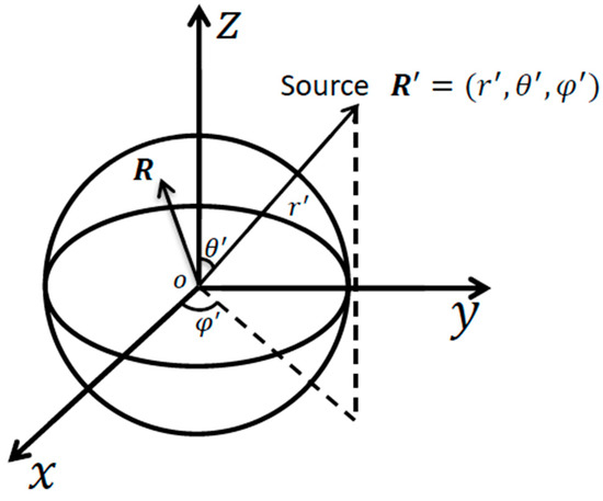
Figure 3. Air-Seawater two-layer model in sphere coordinate system.

Firstly, the vector wave functions in spherical coordinate system are given by [26]

$${\mathit{M}}_{emn}(k)=-\frac{m}{\sin \theta }{z}_n(kr)P_n^m(\cos \theta )\sin m\phi \widehat{\theta }-z_n(kr)\frac{d{P}_n^m(\cos \theta )}{d\theta }\cos m\phi \widehat{\phi },$$

(103)

$${\mathit{M}}_{omn}(k)=\frac{m}{\sin \theta }{z}_n(kr)P_n^m(\cos \theta )\cos m\phi \widehat{\theta }-z_n(kr)\frac{d{P}_n^m(\cos \theta )}{d\theta }\sin m\phi \widehat{\phi },$$

(104)

$$\begin{array}{l}{\mathit{N}}_{emn}(k)=\frac{n(n+1)}{kr}{z}_n(kr)P_n^m(\cos \theta )\cos m\phi \widehat{r}+\frac{1}{kr}\frac{d\left[r{z}_n(kr)\right]}{dr}\cdot \\ \left[\frac{d{P}_n^m(\cos \theta )}{d\theta }\cos m\phi \widehat{\theta }-\frac{m}{\sin \theta }{P}_n^m(\cos \theta )\sin m\phi \widehat{\phi }\right],\end{array}$$

(105)

$$\begin{array}{l}{\mathit{N}}_{omn}(k)=\frac{n(n+1)}{kr}{z}_n(kr)P_n^m(\cos \theta )\sin m\phi \widehat{r}+\frac{1}{kr}\frac{d\left[r{z}_n(kr)\right]}{dr}\cdot \\ \left[\frac{d{P}_n^m(\cos \theta )}{d\theta }\sin m\phi \widehat{\theta }+\frac{m}{\sin \theta }{P}_n^m(\cos \theta )\cos m\phi \widehat{\phi }\right],\end{array}$$

(106)

where $z_n(kr)$ presents $n$ -order spherical Bessel function, $n$ and $m$ indicate the eigenvalue parameters. $k$ denotes the wavenumber. $P_n^m(\cos \theta )$ is a Legendre function of the first type with order $(n,m)$ and it has the following property

$$\underset{\theta \to 0}{\lim }{P}_n^m(\cos \theta )=\{\begin{array}{l}1 m=0\\ 0 else\end{array}.$$

(107)

Similar to the derivation of DGF in cylindrical coordinate system, we can obtain free space DGF in spherical coordinate system

$${\overline{\overline{G}}}_{e2}(\mathit{R},{\mathit{R}}^{’}) =\{\begin{array}{c}-\frac{1}{k}\widehat{r}\widehat{r}\delta (\mathit{R}-{\mathit{R}}^{’})+\frac{\mathrm{i}k}{4\pi }{\displaystyle \sum _{n=0}^{\infty }{\displaystyle \sum _{m=0}^n(2-\delta )}}\frac{2n+1}{n(n+1)}\frac{(n-m)!}{(n+m)!}\cdot \hfill \\ [\mathit{M}(h){\mathit{M}}^{’}(-h)+\mathit{N}(h){\mathit{N}}^{’}(-h)] (z>z^{’})\hfill \\ \hfill \\ -\frac{1}{k}\widehat{r}\widehat{r}\delta (\mathit{R}-{\mathit{R}}^{’})+\frac{\mathrm{i}k}{4\pi }{\displaystyle \sum _{n=0}^{\infty }{\displaystyle \sum _{m=0}^n(2-\delta )}}\frac{2n+1}{n(n+1)}\frac{(n-m)!}{(n+m)!}\cdot \hfill \\ [\mathit{M}(-h){\mathit{M}}^{’}(h)+\mathit{N}(-h){\mathit{N}}^{’}(h)] (z<z^{’})\end{array},$$

(108)

where $\mathit{R}=(r,\theta ,\phi )$ is the position vector of field point and ${\mathit{R}}^{’}=(r^{’},{\theta }^{’},{\phi }^{’})$ denotes the source point.

According to the principle of scattering superposition (96), the DGFs of scattering field can be derived as

$$\begin{array}{l}{\overline{\overline{G}}}_{es}^{(11)}(\mathit{R},{\mathit{R}}^{’})=\frac{\mathrm{i}k}{4\pi }{\displaystyle \sum _{m,n}(2-\delta )}\frac{2n+1}{n(n+1)}\frac{(n-m)!}{(n+m)!}\\ \left[a_2\mathit{M}(k_1){\mathit{M}}^{’}(k_1)+b_2\mathit{N}(k_1){\mathit{N}}^{’}(k_1)\right],\end{array}$$

(109)

$$\begin{array}{l}{\overline{\overline{G}}}_{es}^{(21)}(\mathit{R},{\mathit{R}}^{’})=\frac{\mathrm{i}k}{4\pi }{\displaystyle \sum _{m,n}(2-\delta )}\frac{2n+1}{n(n+1)}\frac{(n-m)!}{(n+m)!}\\ \left[c_2\mathit{M}(k_1){\mathit{M}}^{’}(k_1)+d_2\mathit{N}(k_1){\mathit{N}}^{’}(k_1)\right],\end{array}$$

(110)

where the unknown coefficients $a_2,b_2,c_2,d_2$ can be determined by boundary conditions. For a perfect electromagnetic conductor, since the electric field in the sphere is zero, we can get

$$\begin{array}{l}{a}_2=-\frac{j_n(k_1{r}_a)}{h_n^{(1)}(k_1{r}_a)}, b_2=-\frac{{\left[k_1{r}_a{j}_n(k_1{r}_a)\right]}^{’}}{{\left[k_1{r}_a{h}_n^{(1)}(k_1{r}_a)\right]}^{’}},\\ c_2=0, d_2=0,\end{array}$$

(111)

where $j_n(k_1{r}_a)$ indicates the Bessel function and $h_n^{(1)}(k_1{r}_a)$ is the Hankel function. The radius of the sphere is denoted by $r_a$.

Next, we analyze the expression of the electric field generated by the vertical electric dipole and solve the expression of the electric field by using the DGF in the spherical coordinate system. The derivation is similar to the calculating process in the cylindrical coordinate system and rectangular coordinate system. Therefore, the following part will only focus on the derivation which is obviously different from above.

Suppose the electric dipole is located on the Z-axis and its spherical coordinate is $(d_r,0,0)$. The current source is expressed by

$$\mathit{J}({\mathit{R}}^{’})=I_0\frac{\delta (r^{’}-d_r)\delta ({\theta }^{’})\delta ({\phi }^{’})}{d_r{}^2\sin \theta }\widehat{r},$$

(112)

where $I_0$ stands for the current moment.

The vector wave functions can be simplified

$${\mathit{M}}^{’}{}_{emn}(k)=0,$$

(113)

$${\mathit{M}}^{’}{}_{omn}(k)=0,$$

(114)

$${\mathit{N}}^{’}{}_{e0n}(k)=\frac{n(n+1)}{kr}{z}_n(kr)P_n^0(1)\widehat{r},$$

(115)

$${\mathit{N}}^{’}{}_{o0n}(k)=0.$$

(116)

The simplified DGFs are given by

$$\begin{array}{l}{\overline{\overline{G}}}_e^{(11)}(\mathit{R},{\mathit{R}}^{’})=\frac{\mathrm{i}k}{4\pi }{\displaystyle \sum _{n=1}^{\infty }(2-\delta )}(2n+1)\left[(1+b_2)\mathit{N}(k_1)z_n(kr)P_n^0(1)\widehat{r}\right],\\ {\overline{\overline{G}}}_e^{(21)}(\mathit{R},{\mathit{R}}^{’})=\frac{\mathrm{i}k}{4\pi }{\displaystyle \sum _{n=1}^{\infty }(2-\delta )}(2n+1)\left[d_2\mathit{N}(k_1)z_n(kr)P_n^0(1)\widehat{r}\right].\end{array}$$

(117)

As far as the electric field concerned, it is of course necessary to use (101) and (102). Finally, we get

$$\mathit{E}(\mathit{R})=\{\begin{array}{l}-\frac{k_1\omega {\mu }_0{I}_0}{4\pi (k_1{d}_r)}{\displaystyle \sum _{n=1}^{\infty }(2n+1)}\left[j_n(k_1{d}_r)+b_2{h}_n^{(1)}(k_1{d}_r)\right]{\mathit{N}}_{e0n}^{’}(k_1) r>d_r\\ -\frac{k_1\omega {\mu }_0{I}_0}{4\pi (k_1{d}_r)}{\displaystyle \sum _{n=1}^{\infty }(2n+1)h_n^{(1)}(k_1{d}_r)\left[{\mathit{N}}_{e0n}^{(1)}(k_1)+b_2{\mathit{N}}_{e0n}^{’}(k_1)\right] r<d_r}\end{array}.$$

(118)

In this section, we give the universal form of wave functions in three common coordinates. Combined with the principle of scattering superposition, the DGFs for the two-layer model are proposed. Then the expressions for the electric field are obtained. By observing the electric field of the two-layer model in the three coordinate systems, it can be found that the electric field generated by the vertical electric dipole only contains the TM wave mode. Similar DGFs and electric field expressions are presented in [27], which can confirm the reasonableness of our derivation.

5. Conclusions

We prove that the electric DGF has the property of symmetry and the magnetic DGF is antisymmetric in this paper. What we have investigated mostly above are the DGFs of space rectangular, cylindrical and spherical coordinates. Based on the vector wave functions and the principle of scattering superposition, we propose DGFs in the two-layer model. Furthermore, the DGFs are applied to obtain the electric field generated by a current source. By observing the DGFs of the two-layer model in three coordinate systems, we find that the electric field generated by the vertical electric dipole only contains the TM wave mode. For different research areas, suitable coordinate systems can be used to solve the different problems. For example, the DGF in a cylindrical coordinate system is convenient for cylindrical and circular areas. The DGF in the rectangular coordinate system is more suitable for cuboid and two-dimensional problems. The DGF in the spherical coordinate system has guiding action on superlens technology. In this paper, an effort is made to convince the reader that in this age of supercomputers, theoretical analysis can still contribute a great deal to foster our understanding of the physical processes under consideration.

References

- Levine, H.; Schwinger, J. On the theory of electromagnetic wave diffraction by an aperture in an infinite plane conducting screen. Commun. Pure Appl. Math. 1950, 3, 355–391. [Google Scholar] [CrossRef]
- Azizoglu, S.A.; Koc, S.S.; Buyukdura, O.M. Spherical wave expansion of the time-domain free-space dyadic Green’s function. IEEE Trans. Antennas Propag. 2004, 52, 677–683. [Google Scholar] [CrossRef]
- Bowler, J.R. Time domain half-space dyadic Green’s functions for eddy-current calculations. J. Appl. Phys. 1999, 86, 6494–6500. [Google Scholar] [CrossRef]
- Sphicopoulos, T.; Teodoridis, V.; Gardiol, F.E. Dyadic Green’s function for the electromagnetic field in multilayered isotropic media: An operator approach. IEE Proc. H Microw. Antennas Propag. 2008, 132, 329–334. [Google Scholar] [CrossRef]
- Hanson, G.W. Dyadic Green’s functions for an anisotropic, non-local model of biased graphene. IEEE Trans. Antennas Propag. 2008, 56, 747–757. [Google Scholar] [CrossRef]
- Hui, H.T.; Yung, A.K.N. The eigenfunction expansion of dyadic Green’s functions for chirowave-guides. IEEE Trans. Microw. Theory Tech. 2002, 44, 1575–1583. [Google Scholar]
- Krowne, C.M. Ferrite microstrip circulator 3D dyadic Green’s function with perimeter interfacial walls and internal inhomogeneity. Microw. Opt. Technol. Lett. 1997, 15, 235–242. [Google Scholar] [CrossRef]
- Weiglhofer, W.S. Analytic methods and free-space dyadic Green’s functions. Radio Sci. 1993, 28, 847–857. [Google Scholar] [CrossRef]
- Uno, T. Simplification of dyadic Green’s function for plane stratified inhomogeneous media and its application to lossless DNG slab. Ice Trans. Commun. B 2006, 89, 1661–1671. [Google Scholar]
- Han, F.; Zhuo, J.; Liu, N.; Liu, Y.; Liu, H.; Liu, Q.H. Fast solution of electromagnetic scattering for 3-D inhomogeneous anisotropic objects embedded in layered uniaxial media by the BCGS-FFT method. IEEE Trans. Antennas Propag. 2019, 67, 1748–1759. [Google Scholar] [CrossRef]
- Olyslager, F.; Lindell, I.V. Closed-form Green’s dyadics for a class of media with axial bi-anisotropy. IEEE Trans. Antennas Propag. 1998, 46, 1888–1890. [Google Scholar] [CrossRef]
- Sihvola, A.; Lindell, I.V. Electromagnetic Green Dyadics of Bi-Anisotropic Media in Spectral Domain: The Six-Vector Approach; Rep.244. Electromagnetic Lab.; Helsinki University of Technology: Espoo, Finland, 1997; pp. 1–13. [Google Scholar]
- Li, L.W.; Leong, M.S.; Kooi, P.S.; Yeo, T.S.; Tan, K.H. Rectangular modes and dyadic Green’s functions in a rectangular chirowaveguide. I. Theory. IEEE Trans. Microw. Tech. 1999, 47, 67–73. [Google Scholar]
- Kisliuk, M. The dyadic Green’s functions for cylindrical waveguides and cavities. IEEE Trans. Microw. Tech. 1980, 28, 894–898. [Google Scholar] [CrossRef]
- Engheta, N.; Kowarz, M.W. Antenna radiation in the presence of a Chiral Sphere. Appl. Phys. 1990, 67, 639–647. [Google Scholar] [CrossRef]
- Zhao, M.L.; Zhu, N. A fast preconditioned iterative method for the electromagnetic scattering by multiple cavities with high wave numbers. J. Comput. Phys. 2019, 398, 108826. [Google Scholar] [CrossRef]
- Zhao, M.L.; An, S.; Nie, Y.F. A fast high-order algorithm for the multiple cavity scattering. Int. J. Comput. Math. 2019, 96, 135–157. [Google Scholar] [CrossRef]
- Li, L.W.; Kooi, P.S.; Leong, M.S.; Yeo, T.S. Electromagnetic dyadic Green’s function in spherically multilayered media. IEEE Trans. Microw. Theory Tech. 1994, 42, 2302–2310. [Google Scholar]
- Li, L.W. Dyadic Green’s function of inhomogeneous ionospheric waveguide. J. Electromagn. Waves Appl. 1992, 6, 53–70. [Google Scholar] [CrossRef]
- Song, W.M. A new method for solving dyadic Green’s function of electromagnetic field. J. Electron. 1990, 7, 122–134. [Google Scholar]
- Disfani, M.R.; Vafi, K.; Abrishamian, M.S. Dyadic Green’s function of a PEMC cylinder. Appl. Phys. A 2011, 103, 765–769. [Google Scholar]
- Yin, W.Y.; Wang, W.B. The dyadic Green’s function for the cylindrical chirostrip antenna. Int. J. Infrared Millim. Waves 1993, 14, 849–863. [Google Scholar]
- Dence, D.; Tamir, T. Radio loss of lateral waves in forest environments. Radio Sci. 1969, 4, 307–318. [Google Scholar] [CrossRef]
- Silva, D.K.N.D.; Eras, L.E.C.; Barrsos, F.J.B.; Cavalcante, G.P. VHF–UHF electric field prediction for Amazon city using dyadic Green’s function. Wirel. Pers. Commun. 2020, 113, 1–26. [Google Scholar] [CrossRef]
- Tai, C.T. Dyadic Green’s Functions in Electromagnetic Theory, 2nd ed.; IEEE Press: New York, NY, USA, 1994; pp. 30–47. [Google Scholar]
- Wang, H.L. Study on Electromagnetic Wave Characteristics in Layered Cylindrical and Spherical Media Models. Ph.D. Thesis, Harbin Institute of Technology, Harbin, China, 2008. [Google Scholar]
- Liu, S.D.; Gong, S.G. Antivector Green function method for solving electric dipole electric field in seawater. J. Radio Sci. 2002, 17, 373–377. [Google Scholar]
© 2020 by the authors. Licensee MDPI, Basel, Switzerland. This article is an open access article distributed under the terms and conditions of the Creative Commons Attribution (CC BY) license (http://creativecommons.org/licenses/by/4.0/).