Nonlinear Multigrid Implementation for the Two-Dimensional Cahn–Hilliard Equation

Abstract

We present a nonlinear multigrid implementation for the two-dimensional Cahn–Hilliard (CH) equation and conduct detailed numerical tests to explore the performance of the multigrid method for the CH equation. The CH equation was originally developed by Cahn and Hilliard to model phase separation phenomena. The CH equation has been used to model many interface-related problems, such as the spinodal decomposition of a binary alloy mixture, inpainting of binary images, microphase separation of diblock copolymers, microstructures with elastic inhomogeneity, two-phase binary fluids, in silico tumor growth simulation and structural topology optimization. The CH equation is discretized by using Eyre’s unconditionally gradient stable scheme. The system of discrete equations is solved using an iterative method such as a nonlinear multigrid approach, which is one of the most efficient iterative methods for solving partial differential equations. Characteristic numerical experiments are conducted to demonstrate the efficiency and accuracy of the multigrid method for the CH equation. In the Appendix, we provide C code for implementing the nonlinear multigrid method for the two-dimensional CH equation.

1. Introduction

In this paper, we consider a detailed multigrid [1] implementation of the following two-dimensional Cahn–Hilliard (CH) equation [2] and provide its C source code:

$$\begin{array}{ccc}\hfill \frac{\partial \varphi (x,y,t)}{\partial t}& =& M\mathsf{\Delta }\mu (x,y,t),(x,y)\in \Omega ,t>0,\hfill \\ \hfill \mu (x,y,t)& =& F^{\prime }\left(\varphi (x,y,t)\right)-{ϵ}^2\mathsf{\Delta }\varphi (x,y,t),\hfill \end{array}$$

where $\varphi$ is a conserved scalar field; M is the mobility; $F\left(\varphi \right)=0.25{({\varphi }^2-1)}^2$ is the free energy function (see Figure 1); $ϵ$ is the gradient interfacial energy coefficient; and $\Omega \subset {\mathbb{R}}^2$ is a bounded domain.

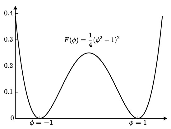
Figure 1. Double-well potential $F\left(\varphi \right)=0.25{({\varphi }^2-1)}^2$.

The homogeneous Neumann boundary conditions are used and are given as follows:

$$\begin{array}{ccc}\hfill \mathbf{n}·\nabla \varphi & =& 0,\hfill \end{array}$$

(1)

$$\begin{array}{ccc}\hfill \mathbf{n}·\nabla \mu & =& 0\mathrm{on}\partial \mathsf{\Omega }.\hfill \end{array}$$

(2)

Here, $\mathbf{n}$ is the unit normal vector on the domain boundary $\partial \mathsf{\Omega }$. The first boundary condition (1) implies that the interface contacts the domain boundary at a ${90}^{°}$ angle. The second boundary condition (2) implies that the total mass is conserved.

We can derive the CH equation from the following total free energy functional

$$\begin{array}{c}\hfill \mathcal{E}\left(\varphi \right)={\int }_{\mathsf{\Omega }}\left[F\left(\varphi \right)+\frac{{ϵ}^2}{2}{|\nabla \varphi |}^2\right]d\mathbf{x}.\end{array}$$

Taking the variational derivative of $\mathcal{E}$ with respect to $\varphi$, we define the chemical potential:

$$\begin{array}{c}\hfill \mu =\frac{\delta \mathcal{E}}{\delta \varphi }=F^{\prime }\left(\varphi \right)-{ϵ}^2\mathsf{\Delta }\varphi .\end{array}$$

Conservation of mass implies the following CH equation

$$\begin{array}{c}\hfill {\varphi }_t=-\nabla ·\mathcal{F},\end{array}$$

where the flux is given by $\mathcal{F}=-M\nabla \mu$. If we differentiate $\mathcal{E}\left(\varphi \right)$ and ${\int }_{\mathsf{\Omega }}\varphi d\mathbf{x}$ with respect to time t, then we have

$$\begin{array}{ccc}\frac{d}{dt}\mathcal{E}\left(\varphi \right)\hfill & =& {\int }_{\mathsf{\Omega }}\left[F^{\prime }\left(\varphi \right){\varphi }_t+{ϵ}^2\nabla \varphi ·\nabla {\varphi }_t\right]\mathrm{d}\mathbf{x}={\int }_{\mathsf{\Omega }}\mu {\varphi }_t\mathrm{d}\mathbf{x}=M{\int }_{\mathsf{\Omega }}\mu \mathsf{\Delta }\mu \mathrm{d}\mathbf{x}\hfill \\ & =& M{\int }_{\partial \mathsf{\Omega }}\mu \nabla \mu ·\mathbf{n}\mathrm{d}s-M{\int }_{\mathsf{\Omega }}\nabla \mu ·\nabla \mu \mathrm{d}\mathbf{x}=-M{\int }_{\mathsf{\Omega }}{|\nabla \mu |}^2\mathrm{d}\mathbf{x}\le 0\hfill \end{array}$$

(3)

and

$$\begin{array}{c}\hfill \frac{d}{dt}{\int }_{\mathsf{\Omega }}\varphi \mathrm{d}\mathbf{x}={\int }_{\mathsf{\Omega }}{\varphi }_t\mathrm{d}\mathbf{x}=M{\int }_{\mathsf{\Omega }}\mathsf{\Delta }\mu \mathrm{d}\mathbf{x}=M{\int }_{\partial \mathsf{\Omega }}\nabla \mu ·\mathbf{n}\mathrm{d}s=0,\end{array}$$

(4)

which imply that the total energy is decreasing and that the total mass is conserved in time, respectively. The CH equation was originally developed by Cahn and Hilliard to model spinodal decomposition in a binary alloy. The CH equation has been used to address many major problems such as the spinodal decomposition of a binary alloy mixture [3,4], inpainting of binary images [5,6], microphase separation of diblock copolymers [7,8], microstructures with elastic inhomogeneity [9,10], two-phase binary fluids [11,12], tumor growth models [13,14,15] and structural topology optimization [14,16]. Further details regarding the basic principles and practical applications of the CH equation are available in a recent review [14]. Thus, knowing how to implement a discrete scheme for the CH equation in detail is very useful because this equation is a building-block equation for many applications. The CH equation is discretized by using Eyre’s unconditionally gradient stable scheme [17] and is solved by using a nonlinear multigrid technique [1], which is one of the most efficient iterative methods for solving partial differential equations. Several studies have used the nonlinear multigrid method for the CH-type equations [18,19,20,21,22,23]. However, details regarding the implementation, multigrid performance, and source codes have not been provided.

Therefore, the main purpose of this paper is to describe a detailed multigrid implementation of the two-dimensional CH equation, evaluate its performance and provide its C programming language source code.

The remainder of this paper is organized as follows. In Section 2, we describe the numerical solution in detail. In Section 3, we describe the characteristic numerical experiments that are conducted to demonstrate the accuracy and efficiency of the multigrid method for the CH equation. In Section 4, we provide a conclusion. In the Appendix A, we provide the C code for implementing the nonlinear multigrid technique for the two-dimensional CH equation.

2. Numerical Solution

We consider a finite difference approximation for the CH equation. An unconditionally gradient energy stable scheme, which was proposed by Eyre, is applied to the time discretization. A nonlinear multigrid technique [1] is applied to solve the resulting system at an implicit time level.

2.1. Discretization

We discretize the CH equation in the two-dimensional space $\mathsf{\Omega }=(a,b)\times (c,d)$. Let $N_x=2^p$ and $N_y=2^q$ be the numbers of mesh points with integers p and q. Let $\mathsf{\Delta }x=(b-a)/N_x$ and $\mathsf{\Delta }y=(d-c)/N_y$ be the mesh size. Let ${\mathsf{\Omega }}_{ij}=\{(x_i,y_j):x_i=a+(i-0.5)\mathsf{\Delta }x,y_j=c+(j-0.5)\mathsf{\Delta }y,1\le i\le N_x,1\le j\le N_y\}$ be a discrete computational domain. Let ${\varphi }_{ij}^n$ and ${\mu }_{ij}^n$ be approximations of $\varphi (x_i,y_j,t_n)$ and $\mu (x_i,y_j,t_n)$, respectively. Here, $t_n=n\mathsf{\Delta }t$ and $\mathsf{\Delta }t$ represent the temporal step. We assume a uniform mesh grid $\mathit{h}=\mathsf{\Delta }x=\mathsf{\Delta }y$ and a constant mobility $M=1$. Using the nonlinear stabilized splitting scheme of Eyre’s unconditionally gradient stable scheme, the CH equation is discretized as

$$\begin{array}{ccc}\hfill \frac{{\varphi }_{ij}^{n+1}-{\varphi }_{ij}^n}{\mathsf{\Delta }t}& =& {\mathsf{\Delta }}_{\mathit{h}}{\mu }_{ij}^{n+1},\hfill \end{array}$$

(5)

$$\begin{array}{ccc}\hfill {\mu }_{ij}^{n+1}& =& {({\varphi }_{ij}^{n+1})}^3-{\varphi }_{ij}^n-{ϵ}^2{\mathsf{\Delta }}_{\mathit{h}}{\varphi }_{ij}^{n+1},\hfill \end{array}$$

(6)

where the discrete Laplace operator is defined by ${\mathsf{\Delta }}_{\mathit{h}}{\psi }_{ij}=({\psi }_{i+1,j}+{\psi }_{i-1,j}+{\psi }_{i,j+1}+{\psi }_{i,j-1}-4{\psi }_{ij})/{\mathit{h}}^2$. The homogeneous Neumann boundary conditions (1) and (2) are discretized as

$$\begin{array}{c}{\varphi }_{0j}={\varphi }_{1j},{\varphi }_{N_x+1,j}={\varphi }_{N_x,j},{\mu }_{0j}={\mu }_{1j},{\mu }_{N_x+1,j}={\mu }_{N_x,j},j=1,\dots ,N_y,\hfill \end{array}$$

(7)

$$\begin{array}{c}{\varphi }_{i0}={\varphi }_{i1},{\varphi }_{i,N_y+1}={\varphi }_{i,N_y},{\mu }_{i0}={\mu }_{i1},{\mu }_{i,N_y+1}={\mu }_{i,N_y},i=1,\dots ,N_x.\hfill \end{array}$$

(8)

We define the discrete residual as

$$\begin{array}{c}\hfill r_{ij}={\mathsf{\Delta }}_{\mathit{h}}{\mu }_{ij}^{n+1}-\frac{{\varphi }_{ij}^{n+1}-{\varphi }_{ij}^n}{\mathsf{\Delta }t}.\end{array}$$

(9)

For each element $a_{ij}$ of size $N_x\times N_y$ in matrix A, we define the Frobenius norm with a scaling and infinite norm as

$$\begin{array}{c}\hfill {∥A∥}_F=\sqrt{\frac{{\sum }_{i=1}^{N_x}{\sum }_{j=1}^{N_y}{\left|a_{ij}\right|}^2}{N_x{N}_y}}\mathrm{and}{∥A∥}_{\infty }=\underset{1\le i\le N_x,1\le j\le N_y}{max}\left|a_{ij}\right|,\end{array}$$

(10)

respectively. The discretizations (5) and (6) are conservative, that is,

$$\begin{array}{c}\hfill \sum _{i=1}^{N_x}\sum _{j=1}^{N_y}{\varphi }_{ij}^{n+1}=\sum _{i=1}^{N_x}\sum _{j=1}^{N_y}{\varphi }_{ij}^n.\end{array}$$

(11)

To show this conservation property, we take the summation of Equation (5)

$$\begin{array}{ccc}\sum _{i=1}^{N_x}\sum _{j=1}^{N_y}\frac{{\varphi }_{ij}^{n+1}-{\varphi }_{ij}^n}{\mathsf{\Delta }t}\hfill & =& \sum _{i=1}^{N_x}\sum _{j=1}^{N_y}{\mathsf{\Delta }}_{\mathit{h}}{\mu }_{ij}^{n+1}\hfill \\ & =& \sum _{j=1}^{N_y}\left(\frac{{\mu }_{N_x+1,j}^{n+1}-{\mu }_{N_{x}j}^{n+1}}{{\mathit{h}}^2}-\frac{{\mu }_{1j}^{n+1}-{\mu }_{0j}^{n+1}}{{\mathit{h}}^2}\right)\hfill \\ & & +\sum _{i=1}^{N_x}\left(\frac{{\mu }_{i,N_y+1}^{n+1}-{\mu }_{i{N}_y}^{n+1}}{{\mathit{h}}^2}-\frac{{\mu }_{i1}^{n+1}-{\mu }_{i0}^{n+1}}{{\mathit{h}}^2}\right)=0.\hfill \end{array}$$

(12)

Here, we used the homogenous Neumann boundary conditions (7) and (8). Therefore, Equation (11) holds. We define the discrete energy functional as

$$\begin{array}{ccc}{\mathcal{E}}^h\left({\varphi }^n\right)\hfill & =& h^2\sum _{i=1}^{N_x}\sum _{j=1}^{N_y}F\left({\varphi }_{ij}^n\right)\hfill \\ & & +\frac{{ϵ}^2}{2}\sum _{j=1}^{N_y}\left(\frac{{({\varphi }_{1j}^n-{\varphi }_{0j}^n)}^2}{2}+\sum _{i=1}^{N_x-1}{({\varphi }_{i+1,j}^n-{\varphi }_{ij}^n)}^2+\frac{{({\varphi }_{N_x+1,j}^n-{\varphi }_{N_{x}j}^n)}^2}{2}\right)\hfill \\ & & +\frac{{ϵ}^2}{2}\sum _{i=1}^{N_x}\left(\frac{{({\varphi }_{i1}^n-{\varphi }_{i0}^n)}^2}{2}+\sum _{j=1}^{N_y-1}{({\varphi }_{i,j+1}^n-{\varphi }_{ij}^n)}^2+\frac{{({\varphi }_{i,N_y+1}^n-{\varphi }_{i{N}_y}^n)}^2}{2}\right)\hfill \\ & =& h^2\sum _{i=1}^{N_x}\sum _{j=1}^{N_y}F\left({\varphi }_{ij}^n\right)+\frac{{ϵ}^2}{2}\sum _{j=1}^{N_y}\sum _{i=1}^{N_x-1}{({\varphi }_{i+1,j}^n-{\varphi }_{ij}^n)}^2+\frac{{ϵ}^2}{2}\sum _{i=1}^{N_x}\sum _{j=1}^{N_y-1}{({\varphi }_{i,j+1}^n-{\varphi }_{ij}^n)}^2,\hfill \end{array}$$

(13)

where we used the homogenous Neumann boundary conditions (7) and (8). We also define the discrete total mass as

$$\begin{array}{c}\hfill {\mathcal{M}}^h\left({\varphi }^n\right)=\sum _{i=1}^{N_x}\sum _{j=1}^{N_y}{\varphi }_{ij}^n{h}^2.\end{array}$$

(14)

Then, the unconditionally gradient stable scheme satisfies the reduction in the discrete total energy [24]:

$$\begin{array}{c}\hfill {\mathcal{E}}^h\left({\varphi }^{n+1}\right)\le {\mathcal{E}}^h\left({\varphi }^n\right),\end{array}$$

(15)

which implies the pointwise boundedness of the numerical solution:

$$\begin{array}{c}\hfill \parallel {\varphi }^n{\parallel }_{\infty }\le \sqrt{1+2\sqrt{{\mathcal{E}}^h\left({\mathit{\varphi }}^0\right)/h^2}}\mathrm{for}\mathrm{all}n.\end{array}$$

(16)

The proof of Equation (16) can be found in Reference [25]. We provide the proof herein for the sake of completeness. We show that a constant K exists for all n values that satisfy the following inequality:

$$\begin{array}{c}\hfill \parallel {\varphi }^n{\parallel }_{\infty }\le K.\end{array}$$

(17)

Let us assume that there is an integer $n_K$ that is dependent on K such that ${\parallel {\varphi }^{n_K}\parallel }_{\infty }>K$ for any K. Then, ${\varphi }_{ij}^{n_K}$ exists such that $|{\varphi }_{ij}^{n_K}|>K$. Let K be the largest solution of ${\mathcal{E}}^h\left({\varphi }^0\right)=h^{2}F\left(K\right)$, that is, $K=\sqrt{1+2\sqrt{{\mathcal{E}}^h\left({\varphi }^0\right)/h^2}}$. We then have

$$\begin{array}{c}\hfill {\mathcal{E}}^h\left({\varphi }^0\right)=h^{2}F\left(K\right)<h^{2}F\left(\right|{\varphi }_{ij}^{n_K}\left|\right)\le {\mathcal{E}}^h\left({\varphi }^{n_K}\right)\le {\mathcal{E}}^h\left({\varphi }^0\right),\end{array}$$

(18)

where we utilize the fact that the total energy is decreasing and $F\left(\varphi \right)$ is a strictly increasing function on $(K,\infty )$. Equation (18) leads to a contradiction. Therefore, Equation (17) should be satisfied.

2.2. Multigrid V-Cycle Algorithm

We use the nonlinear full approximation storage (FAS) multigrid method to solve the nonlinear discrete systems (5) and (6). For simplicity, we define the discrete domains, ${\mathsf{\Omega }}_2,{\mathsf{\Omega }}_1,$ and ${\mathsf{\Omega }}_0$, which represent a hierarchy of meshes (${\mathsf{\Omega }}_2,{\mathsf{\Omega }}_1,$ and ${\mathsf{\Omega }}_0$) created by successively coarsening the original mesh ${\mathsf{\Omega }}_2$, as shown in Figure 2.

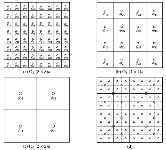
Figure 2. (a–c) represent a sequence of coarse grids starting with $h=L/N_x$. (d) depicts a composition of grids, ${\mathsf{\Omega }}_2,{\mathsf{\Omega }}_1$ and ${\mathsf{\Omega }}_0$.

We summarize here the nonlinear multigrid method for solving the discrete CH system as follows: First, let us rewrite Equations (5) and (6) as

$$\begin{array}{c}\hfill NSO({\varphi }^{n+1},{\mu }^{n+1})=({\xi }^n,{\psi }^n),\end{array}$$

where the linear operator $NSO$ is defined as

$$NSO({\varphi }^{n+1},{\mu }^{n+1})=\left({\varphi }^{n+1}/\mathsf{\Delta }t-{\mathsf{\Delta }}_h{\mu }^{n+1},{\mu }^{n+1}-{\left({\varphi }^{n+1}\right)}^3+{ϵ}^2{\mathsf{\Delta }}_h{\varphi }^{n+1}\right),$$

and the source term is denoted by

$$\begin{array}{c}\hfill \left({\xi }^n,{\psi }^n\right)=\left({\varphi }^n/\mathsf{\Delta }t,-{\varphi }^n\right).\end{array}$$

(19)

Next, we describe the multigrid method, which includes the pre-smoothing, coarse grid correction and post-smoothing steps. We denote a mesh grid ${\mathsf{\Omega }}_k$ as the discrete domain for each multigrid level k. Note that a mesh grid ${\mathsf{\Omega }}_k$ contains $2^k\times 2^k$ grid points. Let $k_{min}$ be the coarsest multigrid level. We now introduce the SMOOTH and V-cycle functions. Given the number ${\nu }_1$ of pre-smoothing and ${\nu }_2$ of post-smoothing relaxation sweeps, the V-cycle is used as an iteration step in the multigrid method.

FAS multigrid cycle

Now, we define the FAScycle:

$$\begin{array}{c}\hfill \{{\varphi }_k^{m+1},{\mu }_k^{m+1}\}=FAScycle(k,{\varphi }_k^m,{\mu }_k^m,NS{O}_k,{\xi }_k^n,{\psi }_k^n,\beta ).\end{array}$$

In other words, $\{{\varphi }_k^m,{\mu }_k^m\}\mathrm{and}\{{\varphi }_k^{m+1},{\mu }_k^{m+1}\}$ are the approximations of ${\varphi }^{n+1}(x_i,y_j)$ and ${\mu }^{n+1}(x_i,y_j)$ before and after an FAScycle, respectively. Here, ${\varphi }_k^0={\varphi }_k^n$ and ${\mu }_k^0={\mu }_k^n$.

(1) Pre-smoothing

$$\begin{array}{c}\hfill \{{\overline{\varphi }}_k^m,{\overline{\mu }}_k^m\}=SMOOT{H}^{{\nu }_1}({\varphi }_k^m,{\mu }_k^m,NS{O}_k,{\xi }_k^n,{\psi }_k^n),\end{array}$$

which represents ${\nu }_1$ smoothing steps with the initial approximations ${\varphi }_k^m,{\mu }_k^m$, source terms ${\xi }_k^n,{\psi }_k^n$ and the $SMOOTH$ relaxation operator to obtain the approximations ${\overline{\varphi }}_k^m,{\overline{\mu }}_k^m.$ One $SMOOTH$ relaxation operator step consists of solving the systems (22) and (23), given as follows by $2\times 2$ matrix inversion for each $i\mathrm{and}j$. Here, we derive the smoothing operator in two dimensions. Rewriting Equation (5), we obtain:

$$\begin{array}{c}\hfill \frac{{\varphi }_{ij}^{n+1}}{\mathsf{\Delta }t}+\frac{4{\mu }_{ij}^{n+1}}{h^2}={\xi }_{ij}^n+\frac{{\mu }_{i+1,j}^{n+1}+{\mu }_{i-1,j}^{n+1}+{\mu }_{i,j+1}^{n+1}+{\mu }_{i,j-1}^{n+1}}{h^2}.\end{array}$$

(20)

Because ${({\varphi }_{ij}^{n+1})}^3$ is nonlinear with respect to ${\varphi }_{ij}^{n+1}$, we linearize ${({\varphi }_{ij}^{n+1})}^3$ at ${\varphi }_{ij}^m$, that is,

$$\begin{array}{c}\hfill {({\varphi }_{ij}^{n+1})}^3\approx {({\varphi }_{ij}^m)}^3+3{({\varphi }_{ij}^m)}^2({\varphi }_{ij}^{n+1}-{\varphi }_{ij}^m).\end{array}$$

After substituting of this into (6), we obtain

$$\begin{array}{c}\hfill -\left(\frac{4{ϵ}^2}{h^2}+3{({\varphi }_{ij}^m)}^2\right){\varphi }_{ij}^{n+1}+{\mu }_{ij}^{n+1}={\psi }_{ij}^n-2{({\varphi }_{ij}^m)}^3-\frac{{ϵ}^2}{h^2}({\varphi }_{i+1,j}^{n+1}+{\varphi }_{i-1,j}^{n+1}+{\varphi }_{i,j+1}^{n+1}+{\varphi }_{i,j-1}^{n+1}).\end{array}$$

(21)

Next, we replace ${\varphi }_{\alpha ,\beta }^{n+1}\mathrm{and}{\mu }_{\alpha ,\beta }^{n+1}$ in Equations (20) and (21) with ${\overline{\varphi }}_{\alpha ,\beta }^m\mathrm{and}{\overline{\mu }}_{\alpha ,\beta }^m$ for $\alpha \le i\mathrm{and}\beta \le j$, otherwise with ${\varphi }_{\alpha ,\beta }^m\mathrm{and}{\mu }_{\alpha ,\beta }^m$, that is,

$$\begin{array}{ccc}\hfill \frac{{\overline{\varphi }}_{ij}^m}{\mathsf{\Delta }t}+\frac{4{\overline{\mu }}_{ij}^m}{h^2}& =& {\xi }_{ij}^n+\frac{{\mu }_{i+1,j}^m+{\overline{\mu }}_{i-1,j}^m+{\mu }_{i,j+1}^m+{\overline{\mu }}_{i,j-1}^m}{h^2},\hfill \end{array}$$

(22)

$$\begin{array}{ccc}\hfill -\left(\frac{4{ϵ}^2}{h^2}+3{({\varphi }_{ij}^m)}^2\right){\overline{\varphi }}_{ij}^m+{\overline{\mu }}_{ij}^m& =& {\psi }_{ij}^n-2{({\varphi }_{ij}^m)}^3-\frac{{ϵ}^2}{h^2}({\varphi }_{i+1,j}^m+{\overline{\varphi }}_{i-1,j}^m+{\varphi }_{i,j+1}^m+{\overline{\varphi }}_{i,j-1}^m).\hfill \end{array}$$

(23)

(2) Compute the defect

$$\begin{array}{c}\hfill ({\overline{d_1^m}}_k,{\overline{d_2^m}}_k)=({\xi }_k^n,{\psi }_k^n)-NS{O}_k({\overline{\varphi }}_k^m,{\overline{\mu }}_k^m).\end{array}$$

(3) Restrict the defect and$\{{\overline{\varphi }}_k^m,{\overline{\mu }}_k^m\}$

$$\begin{array}{c}\hfill ({\overline{d_1}}_{k-1}^m,{\overline{d_2}}_{k-1}^m)=I_k^{k-1}({\overline{d_1}}_k^m,{\overline{d_2}}_k^m).\end{array}$$

The restriction operator $I_k^{k-1}$ maps k-level functions to $(k-1)$-level functions.

$$\begin{array}{ccc}\hfill d_{k-1}(x_i,y_j)=I_k^{k-1}{d}_k(x_i,y_j)& =& \frac{1}{4}[d_k(x_{i-\frac{1}{2}},y_{j-\frac{1}{2}})+d_k(x_{i-\frac{1}{2}},y_{j+\frac{1}{2}})\hfill \\ & & +d_k(x_{i+\frac{1}{2}},y_{j-\frac{1}{2}})+d_k(x_{i+\frac{1}{2}},y_{j+\frac{1}{2}})].\hfill \end{array}$$

(4) Compute the right-hand side

$$\begin{array}{c}\hfill ({\xi }_{k-1}^n,{\psi }_{k-1}^n)=({\overline{d_1^m}}_{k-1},{\overline{d_2^m}}_{k-1})+NS{O}_{k-1}({\overline{\varphi }}_{k-1}^m,{\overline{\mu }}_{k-1}^m).\end{array}$$

(5) Compute an approximate solution $\{{\widehat{\varphi }}_{k-1}^m,{\widehat{\mu }}_{k-1}^m\}$ of the coarse grid equation on ${\mathsf{\Omega }}_{k-1}$, that is,

$$\begin{array}{c}\hfill NS{O}_{k-1}({\varphi }_{k-1}^m,{\mu }_{k-1}^m)=({\xi }_{k-1}^n,{\psi }_{k-1}^n).\end{array}$$

(24)

If $k=1$, we explicitly invert the $2\times 2$ matrix to obtain the solution. If $k>1$, we solve Equation (24) by performing a FAS k-grid cycle using $\{{\overline{\varphi }}_{k-1}^m,{\overline{\mu }}_{k-1}^m\}$ as the initial approximation:

$$\{{\widehat{\varphi }}_{k-1}^m,{\widehat{\mu }}_{k-1}^m\}=\mathrm{FAScycle}(k-1,{\overline{\varphi }}_{k-1}^m,{\overline{\mu }}_{k-1}^m,NS{O}_{k-1},{\xi }_{k-1}^n,{\psi }_{k-1}^n,\beta ).$$

(6) Compute the coarse grid correction (CGC):

$$\begin{array}{c}\hfill {\widehat{v}}_{1k-1}^m={\widehat{\varphi }}_{k-1}^m-{\overline{\varphi }}_{k-1}^m,{\widehat{v}}_{2k-1}^m={\widehat{\mu }}_{k-1}^m-{\overline{\mu }}_{k-1}^m.\end{array}$$

(7) Interpolate the correction:

$$\begin{array}{c}\hfill {\widehat{v}}_{1k}^m=I_{k-1}^k{\widehat{v}}_{1k-1}^m,{\widehat{v}}_{2k}^m=I_{k-1}^k{\widehat{v}}_{2k-1}^m.\end{array}$$

Here, the coarse values are simply transferred to the four nearby fine grid points, that is, $v_k(x_i,y_j)=I_{k-1}^k{v}_{k-1}(x_i,y_j)=v_{k-1}(x_{i+\frac{1}{2}},y_{j+\frac{1}{2}})$ for i and j odd-numbered integers.

(8) Compute the corrected approximation on ${\mathsf{\Omega }}_k$

$$\begin{array}{c}\hfill {\varphi }_k^{m,\mathrm{after}CGC}={\overline{\varphi }}_k^m+{\widehat{v_1}}_k^m,{\mu }_k^{m,\mathrm{after}CGC}={\overline{\mu }}_k^m+{\widehat{v_2}}_k^m.\end{array}$$

(9) Post-smoothing

$$\begin{array}{c}\hfill \{{\varphi }_k^{m+1},{\mu }_k^m\}=SMOOT{H}^{{\nu }_2}({\varphi }_k^{m,\mathrm{after}CGC},{\mu }_k^{m,\mathrm{after}CGC},NS{O}_k,{\xi }_k^n,{\psi }_k^n).\end{array}$$

This completes the description of the nonlinear FAScycle. One FAScycle step stops if the consequent error $\parallel {\varphi }^{n+1,m+1}-{\varphi }^{n+1,m}{\parallel }_{\infty }$ is less than a given tolerance $tol$. The two-grid V-cycle is illustrated in Figure 3.

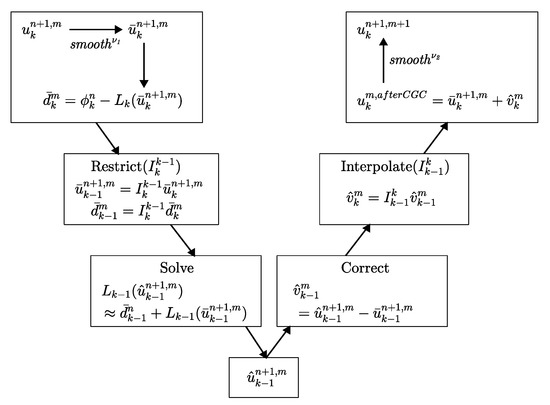
Figure 3. Multigrid two-grid V-cycle method.

Further Numerical Schemes for the CH Equation

Previous studies have described the numerical solution of the CH equation with a variable mobility [19], the adaptive mesh refinement technique [26,27], the Neumann boundary condition in complex domains [20], the Dirichlet boundary conditions in complex domains [28], contact angle boundary [29], parallel multigrid method [30] and fourth-order compact scheme [31].

3. Numerical Experiments

In numerical experiments, we consider an equilibrium solution $\varphi (x,\infty )=tanh(x/\sqrt{2}ϵ)$ for the CH equation on the one-dimensional infinite domain $\mathsf{\Omega }=(-\infty ,\infty )$. In other words, $\varphi (x,\infty )$ satisfies $\mu \left(\varphi (x,\infty )\right)=F^{\prime }\left(\varphi (x,\infty )\right)-{ϵ}^2{\varphi }_{xx}(x,\infty )=0$ and is an equilibrium solution. Then, across the interfacial regions, $\varphi$ varies from $-0.9$ to $0.9$ over a distance of approximately $\xi =2\sqrt{2}ϵ{tanh}^{-1}\left(0.9\right)$ (see Figure 4). Therefore, if we want this value to be approximately $mh$, the $ϵ$ value can be taken as $ϵ={ϵ}_m=mh/\left[2\sqrt{2}{tanh}^{-1}\left(0.9\right)\right]$ [32].

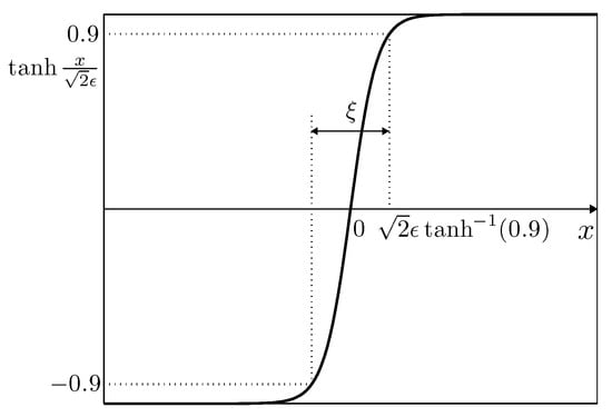
Figure 4. Concentration field varying from $-0.9$ to $0.9$ over a distance of approximately $\xi =2\sqrt{2}ϵ{tanh}^{-1}\left(0.9\right)$.

All computational simulations described in this section are performed on an Intel Core i5-6400 CPU @ 2.70 GHz with 4 GB of RAM.

3.1. Phase Separation

For the first numerical test, we consider spinodal decomposition in binary alloys. This decomposition is a process by which a mixture of binary materials separates into distinct regions with different material concentrations [2]. Figure 5a–c show snapshots of the phase-field $\varphi$ at $t=100\mathsf{\Delta }t$, $200\mathsf{\Delta }t$ and $1000\mathsf{\Delta }t$, respectively. The initial condition is $\varphi (x,y,0)=0.1(1-2\mathrm{rand}(x,y\left)\right)$ on $\mathsf{\Omega }=(0,1)\times (0,1)$, where $\mathrm{rand}(x,y)$ is a random value between 0 and 1. The parameters $ϵ={ϵ}_4$, $h=1/64$, $\mathsf{\Delta }t=0.1h^2$ and a tolerance of $tol$ = $1.0\times {10}^{-10}$ are used.

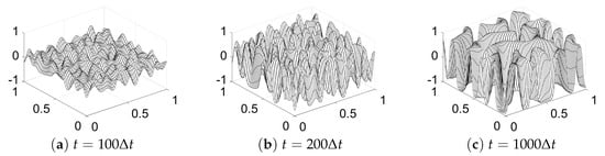
Figure 5. Snapshots of the phase-field $\varphi$ at (a) $t=100\mathsf{\Delta }t$, (b) $t=200\mathsf{\Delta }t$ and (c) $t=1000\mathsf{\Delta }t$. Here, $ϵ={ϵ}_4$, $h=1/64$ and $\mathsf{\Delta }t=0.1h^2$ are used.

3.2. Non-Increase in Discrete Energy and Mass Conservation

Figure 6 shows the time evolution of the normalized discrete total energy ${\mathcal{E}}^h\left({\varphi }^n\right)/{\mathcal{E}}^h\left({\varphi }^0\right)$ (solid line) and the average mass ${\mathcal{M}}^h\left({\varphi }^n\right)/\left(h^2{N}_x{N}_y\right)$ (diamond) of the numerical solutions with the initial state (25) on $\mathsf{\Omega }=(0,1)\times (0,1)$.

$$\begin{array}{c}\hfill \varphi (x,y,0)=0.1(1-2\mathrm{rand}(x,y\left)\right),\end{array}$$

(25)

where $\mathrm{rand}(x,y)$ is a random value between 0 and 1.

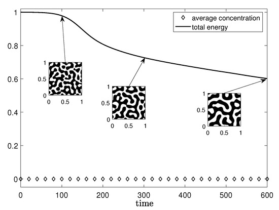
Figure 6. Normalized discrete total energy ${\mathcal{E}}^h\left({\varphi }^n\right)/{\mathcal{E}}^h\left({\varphi }^0\right)$ (solid line) and average concentration ${\mathcal{M}}^h\left({\varphi }^n\right)/\left(h^2{N}_x{N}_y\right)$ (diamond line) of the numerical solutions with the initial state (25).

We use the simulation parameters, $ϵ={ϵ}_4,h=1/64,$$\mathsf{\Delta }t=0.1h^2$ and $tol$ = $1.0\times {10}^{-10}$. The energy is non-increasing and the average concentration is conserved. These numerical results agree well with the total energy dissipation property (3) and the conservation property (4). The inscribed small figures are the concentration fields at the indicated times.

3.3. Convergence Test

We consider the convergence of the Frobenius norm with a scaling of the residual error with respect to the grid size. The initial condition on the domain $\mathsf{\Omega }=(0,1)\times (0,1)$ is given as

$$\begin{array}{c}\hfill \varphi (x,y,0)=0.1cos\left(\pi x\right)cos\left(\pi y\right).\end{array}$$

(26)

We fix $ϵ=0.06$, $\mathsf{\Delta }t=0.01$ and $tol$ = $1.0\times {10}^{-15}$. Here, we use the $V(2,2)$ scheme with a Gauss–Seidel relaxation, where $(2,2)$ indicates 2 pre- and 2 post-correction relaxation sweeps. We define the residual after m V-cycles as

$$\begin{array}{c}\hfill r_{ij}^m={\mathsf{\Delta }}_h{\mu }_{ij}^{n+1,m}-\frac{{\varphi }_{ij}^{n+1,m}-{\varphi }_{ij}^n}{\mathsf{\Delta }t}.\end{array}$$

(27)

Table 1 shows the residual norm ${∥r^m∥}_F$ after each V-cycle. Because no closed-form analytical solution exists for this problem, we define the Frobenius norm with a scaling of the residual error ${∥r^m∥}_F$ = ${∥{\mathsf{\Delta }}_h{\mu }^{n+1,m}-({\varphi }^{n+1,m}-{\varphi }^n)/\mathsf{\Delta }t∥}_F$. The grid sizes are set as $32\times 32$, $64\times 64$ and $128\times 128$. The error norms and ratios of residual between successive V-cycle are shown in Table 1. As we have expected, the residual error decreases successively along with the V-cycle. The sharp increase in the residual norm ratio during the last few cycles reflects the fact that the numerical approximation is already accurate to near machine precision.

Table 1. Error and convergence results for various grid spaces.

Mesh Size	$32\times 32$		$64\times 64$		$128\times 128$
V-Cycle	${∥\mathit{r}∥}_{\mathit{F}}$	Ratio	${∥\mathit{r}∥}_{\mathit{F}}$	Ratio	${∥\mathit{r}∥}_{\mathit{F}}$	Ratio
1	$5.28\times {10}^{-2}$		$6.83\times {10}^{-2}$		$9.10\times {10}^{-2}$
2	$2.41\times {10}^{-3}$	0.05	$3.42\times {10}^{-3}$	0.05	$4.30\times {10}^{-3}$	0.05
3	$1.15\times {10}^{-4}$	0.05	$1.56\times {10}^{-4}$	0.05	$2.09\times {10}^{-4}$	0.05
4	$6.54\times {10}^{-6}$	0.06	$7.25\times {10}^{-6}$	0.05	$8.69\times {10}^{-6}$	0.04
5	$4.23\times {10}^{-7}$	0.06	$4.23\times {10}^{-7}$	0.06	$4.66\times {10}^{-7}$	0.05
6	$2.80\times {10}^{-8}$	0.07	$2.65\times {10}^{-8}$	0.06	$2.90\times {10}^{-8}$	0.06
7	$1.83\times {10}^{-9}$	0.07	$1.58\times {10}^{-9}$	0.06	$1.63\times {10}^{-9}$	0.06
8	$1.23\times {10}^{-10}$	0.07	$1.01\times {10}^{-10}$	0.06	$1.01\times {10}^{-10}$	0.06
9	$8.33\times {10}^{-12}$	0.07	$6.75\times {10}^{-12}$	0.07	$6.83\times {10}^{-12}$	0.07
10	$5.46\times {10}^{-13}$	0.07	$4.24\times {10}^{-13}$	0.06	$4.42\times {10}^{-13}$	0.06
11	$3.70\times {10}^{-14}$	0.07	$4.90\times {10}^{-14}$	0.12	$1.69\times {10}^{-13}$	0.38
12	$1.10\times {10}^{-14}$	$\begin{array}{|c|}\hline 0.30\\ \hline\end{array}$	$4.10\times {10}^{-14}$	$\begin{array}{|c|}\hline 0.84\\ \hline\end{array}$	$1.66\times {10}^{-13}$	$\begin{array}{|c|}\hline 0.98\\ \hline\end{array}$

3.4. Effect of Tolerance

The effect of multigrid tolerance is related to the average mass convergence. We set the initial condition $\varphi (x,y,0)=0.1cos\left(\pi x\right)cos\left(\pi y\right)$ on $\mathsf{\Omega }=(0,1)\times (0,1)$ with tolerance, $tol$ = $1.0\times {10}^{-1}$, $1.0\times {10}^{-2}$, $1.0\times {10}^{-3}$, and $1.0\times {10}^{-10}$ to investigate the relationship between the mass convergence and $tol$. We use the simulation parameters $ϵ={ϵ}_4$, SMOOTH relaxation = 2, $h=1/32$, $\mathsf{\Delta }t=1/32$ and mesh size $32\times 32$. To compare the theoretical value (solid line) with the computational value $tol$ = $1.0\times {10}^{-1}$ (dotted line), $tol$ = $1.0\times {10}^{-2}$ (dash-dot line), $tol$ = $1.0\times {10}^{-3}$ (dashed line) and $tol$ = $1.0\times {10}^{-10}$ (square), we set the interval of average mass from $-0.0019$ to $0.0023$. In Figure 7, the average mass ${\mathcal{M}}^h\left({\varphi }^n\right)/\left(h^2{N}_x{N}_y\right)$ gradually converges to a theoretical value with the decrease in tolerance. In addition, comparing the results of $tol$ = $1.0\times {10}^{-1}$, $1.0\times {10}^{-2}$, $1.0\times {10}^{-3}$ and $1.0\times {10}^{-10}$, we observe that the average mass become nearly convergent for $tol$ = $1.0\times {10}^{-10}$.

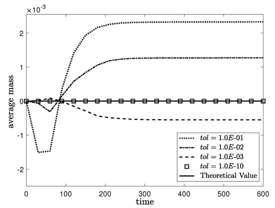
Figure 7. Average mass ${\mathcal{M}}^h\left({\varphi }^n\right)/\left(h^2{N}_x{N}_y\right)$ of the numerical solutions in various values of tolerance. Here, the theoretical value (solid line), $tol$ = $1.0\times {10}^{-1}$ (dotted line), $tol$ = $1.0\times {10}^{-2}$ (dash-dot line), $tol$ = $1.0\times {10}^{-3}$ (dashed line) and $tol$ = $1.0\times {10}^{-10}$ (square).

3.5. Effects of the Smooth Relaxation Numbers ${\nu }_1$ and ${\nu }_2$

We investigate the effects of the SMOOTH relaxation numbers ${\nu }_1$ (pre-relaxation) and ${\nu }_2$ (post-relaxation) on the CPU time. In this test, we perform a numerical simulation with the initial condition $\varphi (x,y,0)=0.1cos\left(\pi x\right)cos\left(\pi y\right)$ on $\mathsf{\Omega }=(0,1)\times (0,1)$, $h=1/128$, ${ϵ}_4$, $\mathsf{\Delta }t=0.1h^2$ and $tol$ = $1.0\times {10}^{-10}$. Table 2 lists the average CPU times and average numbers of V-cycles for various pre- and post-relaxation numbers after 100 time steps. The relaxation numbers are rounded off to the nearest integer. Figure 8 shows the average CPU times for different pre- and post-relaxation numbers. We observe that the average CPU time is the lowest when the numbers of pre- and post-relaxation iterations are ${\nu }_1=2$ and ${\nu }_2=4$, respectively.

Table 2. Average CPU times and average numbers of V-cycles (given in parentheses) for various pre- and post-relaxation numbers after 100 time steps.

$\begin{array}{cc}& {\mathit{\nu }}_1\\ {\mathit{\nu }}_2& \end{array}$	1	2	3	4	5
1	0.075(9)	0.075(7)	0.081(6)	0.077(5)	0.089(5)
2	0.075(7)	0.079(6)	0.090(5)	0.089(5)	0.081(4)
3	0.079(6)	0.082(5)	0.089(5)	0.081(4)	0.090(4)
4	0.078(5)	0.075(4)	0.081(4)	0.090(4)	0.075(3)
5	0.072(4)	0.081(4)	0.090(4)	0.075(3)	0.082(3)

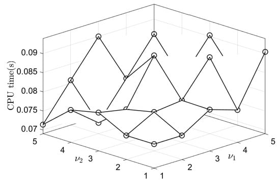
Figure 8. Average CPU time for different pre- and post-relaxation numbers after 100 time steps.

Next, we investigate the effect of SMOOTH relaxation numbers on the finest multigrid level. We perform a numerical simulation with $ϵ=0.0038$ and $\mathsf{\Delta }t$ = $1.0\times {10}^{-7}$. The SMOOTH relaxation numbers ${\nu }_0^1$ and ${\nu }_0^2$ (on the finest multigrid level) are taken to be 1, 2, 3, 4, 5, 6, 7, 8, 9 and 10. In addition, other multigrid levels ${\nu }_k^1={\nu }_k^2$ are $1,2,$ and 3 in the $128\times 128$ and $512\times 512$ mesh sizes. The other parameters are the same as those used previously. Table 3 shows the variations in average CPU time for different relaxation numbers with a $128\times 128$ mesh size. Figure 9 illustrates the results in Table 3.

Table 3. Average CPU times for various relaxation numbers on finest multigrid level (${\nu }_0^1,{\nu }_0^2$) after 10 time steps. In other grids, ${\nu }_k^1={\nu }_k^2,(1\le k)$ relaxation number is fixed at $1,2$ and 3.

$128\times 128$		${\mathit{\nu }}_{\mathit{k}}^1={\mathit{\nu }}_{\mathit{k}}^2$
${\mathit{\nu }}_0^1={\mathit{\nu }}_0^2$	1	2	3
1	0.043	0.049	0.054
2	0.040	0.045	0.048
3	0.027	0.029	0.031
4	0.032	0.034	0.037
5	0.038	0.041	0.042
6	0.044	0.047	0.048
7	0.050	0.053	0.054
8	0.055	0.058	0.060
9	0.062	0.065	0.065
10	0.068	0.070	0.072

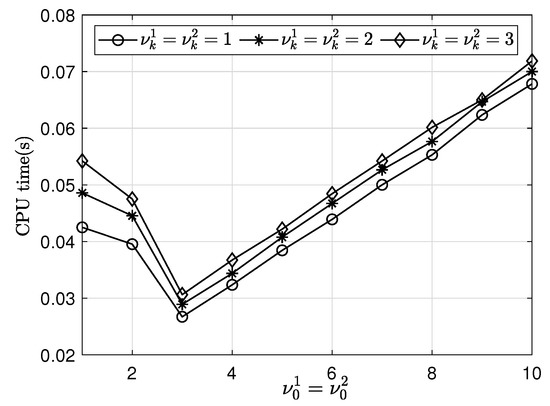
Figure 9. Average CPU times for various relaxation numbers on finest multigrid level (${\nu }_0^1,{\nu }_0^2$) and fixed relaxation number $1,2$ and 3 on other grids with a $128\times 128$ mesh size.

Table 4 lists the variations in average CPU time for different relaxation numbers with a $512\times 512$ mesh size. Figure 10 illustrates the results in Table 4.

Table 4. Average CPU times for various relaxation numbers on finest multigrid level (${\nu }_0^1,{\nu }_0^2$) after 10 time steps. In other grids, the ${\nu }_k^1={\nu }_k^2,(1\le k)$ relaxation number is fixed at $1,2$ and 3.

$512\times 512$		${\mathit{\nu }}_{\mathit{k}}^1={\mathit{\nu }}_{\mathit{k}}^2$
${\mathit{\nu }}_0^1={\mathit{\nu }}_0^2$	1	2	3
1	2.182	2.506	2.750
2	2.030	2.208	2.397
3	1.726	1.850	1.982
4	2.096	2.227	2.351
5	1.872	1.943	2.047
6	2.151	2.236	2.330
7	2.426	2.514	2.617
8	1.817	1.877	1.944
9	2.002	2.066	2.118
10	2.197	2.252	2.295

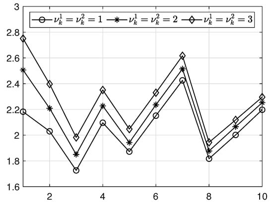
Figure 10. Average CPU times for various relaxation numbers on finest multigrid level (${\nu }_0^1,{\nu }_0^2$) and fixed relaxation numbers $1,2$ and 3 on other grids with a $512\times 512$ mesh size.

3.6. Effect Of V-Cycle

Next, we investigate the effect of V-cycle by changing the multigrid levels. In this test, we use the parameters $\mathsf{\Delta }t=0.01$, $ϵ=0.06$, SMOOTH relaxation $=2$, $tol=1.0\times {10}^{-10}$ and $h=1/128$ on $\mathsf{\Omega }=(0,1)\times (0,1)$ with a initial condition $\varphi (x,y,0)=0.1cos\left(\pi x\right)cos\left(\pi y\right)$. The highest number of V-cycles is taken to be 10000. We use $leve{l}_2$, $leve{l}_3$, $leve{l}_4$, $leve{l}_5$, $leve{l}_6$ and $leve{l}_7$ in a single time step as examples to illustrate the effect of the V-cycle. We calculate the CPU time for each level after 100$\mathsf{\Delta }t$, as listed in Table 5.

Table 5. Numbers of multigrid levels and CPU times required until tolerance ≤$1.0\times {10}^{-10}$. Here, different levels are used.

Level	2	3	4	5	6	7
CPU time(s)	1271.437	342.906	103.032	66.422	66.172	65.218

The number of the multigrid level and CPU time shown in Figure 11 indicate that a greater number of the multigrid level leads to a obvious decrease in CPU time. It is important to select an appropriate multigrid level for a specific mesh size.

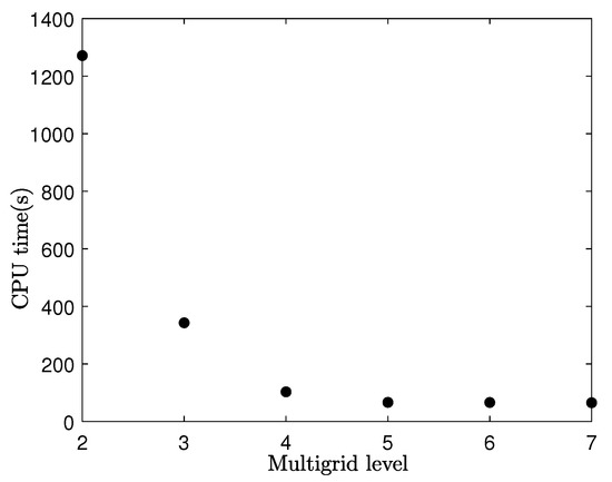
Figure 11. Required CPU times in various multigrid levels after 100 time steps.

3.7. Comparison between Gauss–Seidel and Multigrid Algorithms

We compare the average CPU times required to perform the Gauss–Seidel algorithm and multigrid algorithm. In this test, the initial condition is taken to be $\varphi (x,y,0)=cos\left(\pi x\right)cos\left(\pi y\right)$. The following parameters are used—$\mathsf{\Delta }t=0.01$, $T=10\mathsf{\Delta }t$, the SMOOTH relaxation $=2$ and $ϵ=0.06$. The highest number of V-cycle is taken to be 10000. The mesh sizes are $32\times 32$, $64\times 64$ and $128\times 128$. The tolerances are $1.0\times {10}^{-3}$, $1.0\times {10}^{-4}$ and $1.0\times {10}^{-5}$. Table 6 shows the average CPU times for these two methods after 10 time steps. We observe that the multigrid method require less CPU time than the Gauss–Seidel method does.

Table 6. Average CPU times for Gauss–Seidel and multigrid algorithms with different tolerances after 10 time steps.

Mesh Size	$tol$	Gauss–Seidel	Multigrid
	$1.0\times {10}^{-3}$	0.468	0.046
$32\times 32$	$1.0\times {10}^{-4}$	0.610	0.063
	$1.0\times {10}^{-5}$	0.735	0.062
	$1.0\times {10}^{-3}$	7.046	0.203
$64\times 64$	$1.0\times {10}^{-4}$	8.984	0.234
	$1.0\times {10}^{-5}$	11.360	0.266
	$1.0\times {10}^{-3}$	109.093	0.844
$128\times 128$	$1.0\times {10}^{-4}$	140.219	0.906
	$1.0\times {10}^{-5}$	174.922	1.078

3.8. Effects of $tol$ and $\mathsf{\Delta }t$ on the V-Cycle

In this test, we study the effects of $tol$ and $\mathsf{\Delta }t$ on the V-cycle with the initial condition being $\varphi (x,y,0)=0.1cos\left(\pi x\right)cos\left(\pi y\right)$, $h=1/128,ϵ=0.06$. The highest number of the V-cycle is taken to be 10,000. Table 7 shows the number of V-cycle for various $tol$ and $\mathsf{\Delta }t$ after a single time step. We can find that lower values of $tol$ lead to an increase in the V-cycle. For different values of $tol$, it is essential to choose an appropriate $\mathsf{\Delta }t$ to reduce the number of V-cycle.

Table 7. Numbers of V-cycles for various $tol$ and $\mathsf{\Delta }t$ after a single time step.

$\begin{array}{cc}& \mathbf{\Delta }\mathit{t}\\ \mathit{t}\mathit{o}\mathit{l}& \end{array}$	${10}^{-7}{\mathit{h}}^2$	${10}^{-6}{\mathit{h}}^2$	${10}^{-5}{\mathit{h}}^2$	${10}^{-4}{\mathit{h}}^2$	${10}^{-3}{\mathit{h}}^2$	${10}^{-2}{\mathit{h}}^2$	${10}^{-1}{\mathit{h}}^2$
$1.0\times {10}^{-5}$	2	2	3	4	6	8	8
$1.0\times {10}^{-6}$	10,000	2	3	4	7	9	9
$1.0\times {10}^{-7}$	10,000	10,000	3	5	8	10	10
$1.0\times {10}^{-8}$	10,000	10,000	10,000	5	9	11	12
$1.0\times {10}^{-9}$	10,000	10,000	10,000	10,000	10	13	13
$1.0\times {10}^{-10}$	10,000	10,000	10,000	10,000	10,000	14	15
$\begin{array}{cc}& \mathbf{\Delta }\mathit{t}\\ \mathit{t}\mathit{o}\mathit{l}& \end{array}$	${\mathit{h}}^2$	$10{\mathit{h}}^2$	${10}^2{\mathit{h}}^2$	${10}^3{\mathit{h}}^2$	${10}^4{\mathit{h}}^2$	${10}^5{\mathit{h}}^2$	${10}^6{\mathit{h}}^2$
$1.0\times {10}^{-5}$	8	7	8	8	9	14	41
$1.0\times {10}^{-6}$	9	9	9	9	10	19	91
$1.0\times {10}^{-7}$	11	10	10	11	11	24	140
$1.0\times {10}^{-8}$	12	12	12	12	13	28	189
$1.0\times {10}^{-9}$	14	13	13	13	14	33	238
$1.0\times {10}^{-10}$	15	14	15	15	16	38	288

3.9. Comparison of the Jacobi, Red–Black and Gauss–Seidel

We compare the performance of three relaxation methods: Jacobi, Red–Black and Gauss–Seidel. The initial condition is $\varphi (x,y,0)=0.1cos\left(\pi x\right)cos\left(\pi y\right)$ on $\mathsf{\Omega }=(0,1)\times (0,1)$. The parameters are $h=1/128$, $ϵ=0.06$, $\mathsf{\Delta }t={10}^{-7}$, $T=100\mathsf{\Delta }t$ and $tol=1.0\times {10}^{-10}$. The SMOOTH relaxation numbers on the finest multigrid level (i.e., ${\nu }^1={\nu }^2$) are taken to be from 1 to 5 and those on the other multigrid levels are selected as 2 with the $128\times 128$ mesh size. The relaxation numbers are rounded off to the nearest integer. Table 8 shows the average number of V-cycles for different relaxation numbers with the three methods. The relationship between the average numbers of V-cycles and ${\nu }^1={\nu }^2$ with the Jacobi, Red–Black and Gauss–Seidel method is plotted in Figure 12. The Gauss–Seidel method is observed to be the fastest. In the parallel multigrid method, the relaxation options are either Jacobi or Red–Black [33]. The Jacobi method requires approximately twice as many V-cycles as the Red–Black method does.

Table 8. Average numbers of V-cycles for various relaxation numbers. The SMOOTH relaxation numbers on the finest multigrid level (i.e., ${\nu }^1={\nu }^2$) are taken to be from 1 to 5.

Case	Jacobi	Red–Black	Gauss-Seidal
1	32	13	9
2	16	8	6
3	11	6	5
4	8	5	4
5	7	5	3

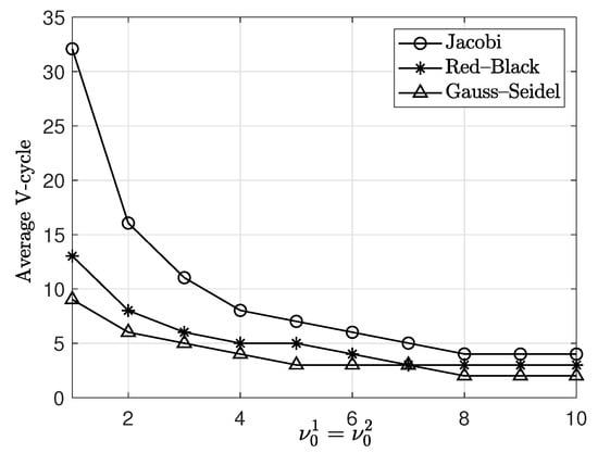
Figure 12. Plot of the average numbers of V-cycles versus ${\nu }^1={\nu }^2$ with the Jacobi (○), Red–Black (∗) and Gauss–Seidel (△) method.

3.10. Effect of $ϵ$

Next, we investigate the effect of $ϵ={ϵ}_m$, which is related to the interface width. In this test, we perform a numerical simulation with the initial condition

$$\begin{array}{c}\hfill \varphi (x,y,0)=\left\{\begin{array}{c}\begin{array}{cc}\hfill 1& \mathrm{if}0.15\le x\le 0.85\mathrm{and}0.15\le y\le 0.85,\hfill \\ \hfill -1& \mathrm{otherwise},\hfill \end{array}\hfill \end{array}\right.\end{array}$$

on $\mathsf{\Omega }=(0,1)\times (0,1)$. We use $h=1/128$, $\mathsf{\Delta }t=h$, SMOOTH relaxation $=2$, $tol=1.0\times {10}^{-10}$ and $T=1000\mathsf{\Delta }t$. Figure 13 presents the evolution of the CH equation with the three values ${ϵ}_4$, ${ϵ}_8$ and ${ϵ}_{16}$. As we have expected, the lower value of $ϵ$ leads to a narrower interface width.

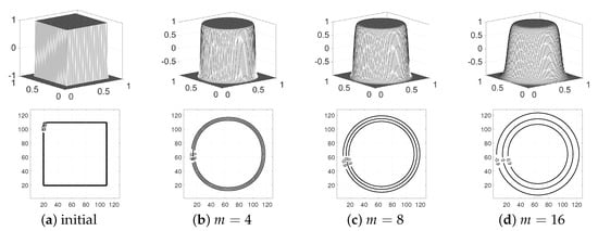
Figure 13. Evolution of the Cahn–Hilliard (CH) equation with different $ϵ={ϵ}_m$: (a) initial condition, (b–d) $m=4$, $m=8$ and $m=16$ at $T=1000\mathsf{\Delta }t$, respectively.

3.11. Effect of mesh size, $N_x\times N_y$

In this test, we compare the CPU times with different mesh sizes $N_x\times N_y$. The initial condition is $\varphi (x,y,0)=0.1cos\left(\pi x\right)cos\left(\pi y\right)$ on $\mathsf{\Omega }=(0,N_x/32)\times (0,N_y/32)$. The parameters are $h=1/32$, $\mathsf{\Delta }t=h$, $T=100\mathsf{\Delta }t$, $ϵ=0.06$, SMOOTH relaxation $=2$ and $tol=1.0\times {10}^{-10}$. Table 9 shows the CPU times and their ratios (that is, the ratio of the CPU time with the mesh size $2N_x\times 2N_y$ to the CPU time with $N_x\times N_y$). We observe that the values converge to 4.

Table 9. CPU times for different mesh sizes.

Mesh Size	$32\times 32$		$64\times 64$		$128\times 128$		$256\times 256$
CPU time(s)	0.610		2.812		12.156		50.594
Ratio		4.610		4.323		4.162

4. Conclusions

In this paper, we presented a nonlinear multigrid implementation for the CH equation in a two-dimensional space. Eyre’s unconditionally gradient stable scheme was used to discretize the governing equation. The resulting discretizing equations were solved using the nonlinear multigrid method. We described the implementation of our numerical scheme in detail. We numerically showed the decrease in discrete total energy and the convergence of discrete total mass. We took a convergence test by studying the reductions in residual error on various mesh sizes in a single time step. The results of various numerical experiments were presented to demonstrate the effects of tolerance, SMOOTH relaxation, V-cycle and $ϵ$. The provided multigrid source code will be useful to beginners who needs the numerical implementation of the nonlinear multigrid method for the CH equation.

References

- Trottenberg, U.; Schüller, A.; Oosterlee, C.W. Multigrid Methods; Academic Press: Cambridge, MA, USA, 2000. [Google Scholar]
- Cahn, J.W.; Hilliard, J.E. Free energy of a nonuniform system. I. Interfacial free energy. J. Chem. Phys. 1958, 28, 258–267. [Google Scholar]
- Copetti, M.I.M.; Elliott, C.M. Kinetics of phase decomposition processes: Numerical solutions to Cahn–Hilliard equation. Mater. Sci. Technol. 1990, 6, 273–284. [Google Scholar]
- Honjo, M.; Saito, Y. Numerical simulation of phase separation in Fe-Cr binary and Fe-Cr-Mo ternary alloys with use of the Cahn–Hilliard equation. ISIJ Int. 2000, 40, 914–919. [Google Scholar]
- Bertozzi, A.L.; Esedoglu, S.; Gillette, A. Inpainting of binary images using the Cahn–Hilliard equation. IEEE Trans. Image Process. 2007, 16, 285–291. [Google Scholar]
- Bosch, J.; Kay, D.; Stoll, M.; Wathen, A.J. Fast solvers for Cahn–Hilliard inpainting. SIAM J. Imaging Sci. 2014, 7, 67–97. [Google Scholar]
- Choksi, R.; Peletier, M.A.; Williams, J.F. On the phase diagram for microphase separation of diblock copolymers: An approach via a nonlocal Cahn–Hilliard functional. SIAM J. Appl. Math. 2009, 69, 1712–1738. [Google Scholar]
- Tang, P.; Qiu, F.; Zhang, H.; Yang, Y. Phase separation patterns for diblock copolymers on spherical surfaces: A finite volume method. Phys. Rev. E 2005, 72, 016710. [Google Scholar]
- Hu, S.Y.; Chen, L.Q. A phase-field model for evolving microstructures with strong elastic inhomogeneity. Acta Mater. 2001, 49, 1879–1890. [Google Scholar]
- Yu, P.; Hu, S.Y.; Chen, L.Q.; Du, Q. An iterative-perturbation scheme for treating inhomogeneous elasticity in phase-field models. J. Comput. Phys. 2005, 208, 34–50. [Google Scholar]
- Gurtin, M.E.; Polignone, D.; Vinals, J. Two-phase binary fluids and immiscible fluids described by an order parameter. Math. Models Methods Appl. Sci. 1996, 6, 815–831. [Google Scholar]
- Lee, T. Effects of incompressibility on the elimination of parasitic currents in the lattice Boltzmann equation method for binary fluids. Comput. Math. Appl. 2009, 58, 987–994. [Google Scholar]
- Jeong, D.; Kim, J. Phase-field model and its splitting numerical scheme for tissue growth. Appl. Numer. Math. 2017, 117, 22–35. [Google Scholar]
- Kim, J.; Lee, S.; Choi, Y.; Lee, S.M.; Jeong, D. Basic Principles and Practical Applications of the Cahn–Hilliard Equation. Math. Probl. Eng. 2016, 2016, 9532608. [Google Scholar]
- Colli, P.; Gilardi, G.; Sprekels, J. A distributed control problem for a fractional tumor growth model. Mathematics 2019, 7, 792. [Google Scholar]
- Myśliński, A.; Wroblewski, M. Structural optimization of contact problems using Cahn–Hilliard model. Comput. Struct. 2017, 180, 52–59. [Google Scholar]
- Eyre, D.J. Unconditionally gradient stable time marching the Cahn–Hilliard equation. MRS Proc. 1998, 529, 39. [Google Scholar]
- Yang, S.; Lee, H.; Kim, J. A phase-field approach for minimizing the area of triply periodic surfaces with volume constraint. Comput. Phys. Commun. 2010, 181, 1037–1046. [Google Scholar]
- Kim, J. A numerical method for the Cahn–Hilliard equation with a variable mobility. Commun. Nonlinear Sci. Numer. Simul. 2007, 12, 1560–1571. [Google Scholar]
- Shin, J.; Jeong, D.; Kim, J. A conservative numerical method for the Cahn–Hilliard equation in complex domains. J. Comput. Phys. 2011, 230, 7441–7455. [Google Scholar]
- Jeong, D.; Kim, J. A practical numerical scheme for the ternary Cahn–Hilliard system with a logarithmic free energy. Phys. A 2016, 442, 510–522. [Google Scholar]
- Lee, H.; Kim, J. A second-order accurate non-linear difference scheme for the N-component Cahn–Hilliard system. Phys. A 2008, 387, 4787–4799. [Google Scholar]
- Lee, H.G.; Shin, J.; Lee, J.Y. A High-Order Convex Splitting Method for a Non-Additive Cahn–Hilliard Energy Functional. Mathematics 2019, 7, 1242. [Google Scholar]
- Shin, J.; Choi, Y.; Kim, J. An unconditionally stable numerical method for the viscous Cahn–Hilliard equation. Discret. Contin. Dyn. Syst. Ser. B 2014, 19, 1737–1747. [Google Scholar]
- Kim, J. Phase-field models for multi-component fluid flows. Commun. Comput. Phys. 2012, 12, 613–661. [Google Scholar]
- Kim, J.; Bae, H.O. An unconditionally gradient stable adaptive mesh refinement for the Cahn–Hilliard equation. J. Korean Phys. Soc. 2008, 53, 672–679. [Google Scholar]
- Wise, S.; Kim, J.; Lowengrub, J. Solving the regularized, strongly anisotropic Cahn–Hilliard equation by an adaptive nonlinear multigrid method. J. Comput. Phys. 2007, 226, 414–446. [Google Scholar]
- Li, Y.; Jeong, D.; Shin, J.; Kim, J. A conservative numerical method for the Cahn–Hilliard equation with Dirichlet boundary conditions in complex domains. Comput. Math. Appl. 2013, 65, 102–115. [Google Scholar]
- Lee, H.G.; Kim, J. Accurate contact angle boundary conditions for the Cahn–Hilliard equations. Comput. Fluids 2011, 44, 178–186. [Google Scholar]
- Shin, J.; Kim, S.; Lee, D.; Kim, J. A parallel multigrid method of the Cahn–Hilliard equation. Comput. Mater. Sci. 2013, 71, 89–96. [Google Scholar]
- Lee, C.; Jeong, D.; Shin, J.; Li, Y.; Kim, J. A fourth-order spatial accurate and practically stable compact scheme for the Cahn–Hilliard equation. Phys. A 2014, 409, 17–28. [Google Scholar]
- Choi, J.W.; Lee, H.G.; Jeong, D.; Kim, J. An unconditionally gradient stable numerical method for solving the Allen–Cahn equation. Phys. A 2009, 388, 1791–1803. [Google Scholar]
- Baker, A.H.; Falgout, R.D.; Kolev, T.V.; Yang, U.M. Scaling hypre’s multigrid solvers to 100,000 cores. In High-Performance Scientific Computing; Springer: London, UK, 2012; pp. 261–279. [Google Scholar]
© 2020 by the authors. Licensee MDPI, Basel, Switzerland. This article is an open access article distributed under the terms and conditions of the Creative Commons Attribution (CC BY) license (http://creativecommons.org/licenses/by/4.0/).