FCS-MBFLEACH: Designing an Energy-Aware Fault Detection System for Mobile Wireless Sensor Networks

Abstract

Wireless sensor networks (WSNs) include large-scale sensor nodes that are densely distributed over a geographical region that is completely randomized for monitoring, identifying, and analyzing physical events. The crucial challenge in wireless sensor networks is the very high dependence of the sensor nodes on limited battery power to exchange information wirelessly as well as the non-rechargeable battery of the wireless sensor nodes, which makes the management and monitoring of these nodes in terms of abnormal changes very difficult. These anomalies appear under faults, including hardware, software, anomalies, and attacks by raiders, all of which affect the comprehensiveness of the data collected by wireless sensor networks. Hence, a crucial contraption should be taken to detect the early faults in the network, despite the limitations of the sensor nodes. Machine learning methods include solutions that can be used to detect the sensor node faults in the network. The purpose of this study is to use several classification methods to compute the fault detection accuracy with different densities under two scenarios in regions of interest such as MB-FLEACH, one-class support vector machine (SVM), fuzzy one-class, or a combination of SVM and FCS-MBFLEACH methods. It should be noted that in the study so far, no super cluster head (SCH) selection has been performed to detect node faults in the network. The simulation outcomes demonstrate that the FCS-MBFLEACH method has the best performance in terms of the accuracy of fault detection, false-positive rate (FPR), average remaining energy, and network lifetime compared to other classification methods.

1. Introduction

Wireless sensor networks (WSNs) are one of the most prominent tools for information acquisition and understanding of the region that has led to extensive research [1]. WSNs include a number of sensor nodes that are typically small and inexpensive. Much progress in the field of wireless communication systems and digital electronics technology has occurred, expanding the use of small-size multipurpose sensor nodes. In most applications of wireless sensor networks, the nodes are randomly located in a physical region, and there is no specific, predetermined map. Sensor nodes automatically compose the sensor network structure after being placed in the region. These networks interact severely with the physical region. It is possible to collect information on wireless sensor networks through the collaborative work of sensor nodes without human intervention. In a wireless sensor network, the radius of data transmission is determined by the radio frequency. Each sensor node communicates with its neighboring sensor nodes in the network so that the memory, computing power, and energy resources for this node are limited [2].

One of the crucial difficulties in advancing the wireless sensor networks is that power supplies are significantly narrower than wired networks, causing sensor nodes to consume energy when receiving, processing, and transmitting information to other nodes in a WSN, and the energy required to do so is provided by the batteries embedded in each node independently. WSNs are typically located in high-risk regions where it is almost impossible to recharge or replace the battery. The performance of these networks is severely dependent on the network’s lifetime and the scale of its coverage. The use of energy-aware algorithms in the design of long-life sensor networks is crucial [3].

Therefore, the lifetime of the network is completely dependent on the power source of its sensor nodes. This limitation creates problems that are the origin of many research debates regarding nodes’ lifetime and energy consumption. To preserve energy in sensor nodes, a cluster-based approach has been developed in which only some nodes are allowed to communicate with the base station to save energy. Selecting a suitable cluster head (CH) is one of the solutions that can saliently reduce energy consumption. Clustering improves the scalability of the wireless sensor network. This is the reason that clustering minimizes the direct dependence of the sensor nodes on the base station and numerous traffic loads, as well as expands local decision making for transmitting information.

Considering that the purpose of this study is to detect the fault in a distributed system, the presence of a fault in wireless sensor data may increase network traffic, communication overhead, and reduce the fault detection efficiency for the base station, and eventually lead to the loss of battery power, high energy consumption, and decreased network lifetime. Faults should be detected early to optimally preserve battery power. So, fault detection is associated with the energy consumption of sensor nodes in the network, which is a crucial cluster head selection approach for optimizing energy consumption.

In this study, the MB-FLEACH algorithm [4] was used to select the cluster head according to the scenarios defined in [4] for the proposed method, which is called FCS-MBFLEACH.

The proposed FCS-MBFLEACH method has been compared with MB-FLEACH, one support vector machine (SVM), and fuzzy one SVM methods in terms of the false-positive rate (FPR), the accuracy of fault detection, the average of the remaining energy, and the network lifetime.

Other sections of the article are organized as follows. The second section deals with related work. The third section includes a discussion of the proposed algorithm and other classification algorithms. The fourth section contains the experiments, and in the fifth section, we evaluate the results. Finally, the sixth section describes the conclusions and future research work.

2. Related Works

Fault detection in wireless sensor networks has been accomplished with many research efforts in a variety of ways, including centralized detection, distributed, and hybrid detection [5]. In general, for a low-traffic small-scale load, the centralized fault detection method is very effective. However, using this method creates a bottleneck due to the dependence of the sensor nodes to a central node, in which the node density is too high to capture information resources. In this situation, the scalability of the system will decrease. However, for large-scale wireless networks, due to the limitations of sensor nodes, the distributed fault detection method is used to reduce the energy consumption, increase the network lifetime, and reduce the traffic load in the network. In the distributed fault detection method, the decision is made to detect locally so that each node conducts the fault detection function independently. Therefore, the measure of information generated by the data sent to the central node is further reduced. It also reduces the energy consumption and congestion of the network; in addition, it increases the lifetime of the entire network [6,7]. Finally, a hybrid method for fault detection consisting of the statistic with the neighborhood and multi-tiered methods [5].

Since the purpose of this study is to detect the distributed fault, we review recent works done by researchers on distributed methods.

Chen et al. [6] have presented a distributed fault detection (DFD) algorithm for wireless sensor networks that determines the initial state of the sensor node, whether it has a fault or not. They use mutual testing of the relevant node and its node neighbors using the DFD algorithm. In fact, the final state of the node is determined based on the initial state of the sensor node. The advantages of this algorithm are its higher detection accuracy and lower fault alarm rate. The disadvantage of this algorithm is that it requires at least two interconnections between neighboring nodes, which results in high energy consumption. In another research, Jiang in [8] proposed an improved distributed fault detection algorithm. If the number of neighboring nodes and the failure rate are high, the fault detection accuracy is reduced in traditional distributed fault detection, and the complexity and energy consumption are increased. However, he improved the traditional DFD algorithm by refining the fault detection criterion to identify the final state of the node so that the false alarm rate was reduced. It also increased the accuracy of fault detection. However, the problem of high energy consumption is one of the challenges of this algorithm. Kai and Li in [9] suggested a cluster-based fault detection algorithm to detect the fault nodes from the cluster head node in the target cluster and employed the optimum threshold value to improve the fault detection accuracy and reduced the effect on the fault nodes according to the probability of sensor node fault. However, there is still the problem of high energy consumption in this algorithm. Feng et al. [10] proposed a distributed fault detection method based on weighted distance. To evaluate the fault nodes, their measured value of a sensor node is compared with the initial measured value. The weighted distance between a node and its neighbor node is computed. Then, the obtained value is compared with the value of the original data with a fixed parameter. If this value is less than its parameter value, then the node is safe; otherwise, it is faulty.

A distributed algorithm called distributed self-fault diagnosis (DSFD) by Panda and Khilar based on a modified three-sigma edit test [11] was proposed to detect the soft and hard faults [12]. The DFSD algorithm conducts a normal workload for a node to determine its status. In this algorithm, each node can learn its own fault status by gathering information from neighboring nodes, and then the node status is checked. If the sensor node detects its own status as a fault, then it is stopped in network activity. However, if the density of the node increases, the network performance for fault detection by the node is reduced.

Another algorithm called low energy consumption distributed fault detection (LEDFD) was proposed by Xu et al. in [13], which uses the temporal correlation characteristics of the data collected to detect some fault nodes and eliminates them. This algorithm reduces the communication time between the sensor nodes, and it reduces the energy consumption in the network. It also uses spatial characteristics to detect the remaining fault nodes that were not detected in the previous diagnosis. If the measured value of the nodes is similar or close to the measured value of the neighboring nodes so that its previous state is normal for the node, then the node is considered to be a safe node. However, in this system, as the node density increases, the network performance decreases.

Artail et al. in [14] proposed a distributed fault detection method based on the clustering structure in a sensor network. In this method, a Markov chain controller is used to detect the fault node in a base station so that in each cluster is used for data exchange between cluster heads (CHs) and neighboring cluster head nodes to complete the cluster head fault detection. In this clustering method, the cluster head node is responsible for data transmission, fault detection, and the location of the sensor nodes.

Hosseini et al. [4] proposed the MB-FLEACH algorithm for selecting a super cluster head in wireless sensor networks to optimize energy consumption reduction and increase the network lifetime. In fact, the purpose of this algorithm is to reduce energy consumption and increase network lifetime by assuming that the base station is mobile and it moves in different time rounds. The computational complexity of this algorithm is very low. However, using this algorithm, node fault detection is not performed.

Saeedi and Mazinani in [15] used SVM and a density-based spatial clustering of applications with noise (DBSCAN) algorithms to detect anomalies in wireless sensor networks. They use the DBSCAN algorithm to detect anomalies in low-density data points in the network, and they use SVM to improve detection accuracy. They did not compute the measure of the remaining energy after the fault detection in their study. Other studies in [16,17] also used SVM-based methods to detect anomalies in wireless sensor networks.

Cheng et al. [7] proposed a distributed fault detection algorithm based on support vector regression for wireless sensor networks, which is a fault detection mechanism based on support vector regression and neighbors’ collaboration. Based on the data collected by several sensors, the fault prediction model is constructed using the SVM regression algorithm, and thus the remaining sequences are obtained. Then, the status of the node—whether it has a fault or not—is determined by mutual testing between valid neighbor nodes. The proposed algorithm is suitable for low-density nodes with a high failure rate. It also reduces the network traffic created by the sensor nodes and increases the accuracy of fault detection.

Therefore, according to the literature review, data-based learning classification methods and statistical learning techniques can quickly determine the fault data points for different classes.

One of these methods is the SVM; because it provides an optimal solution for data classification, the algorithm is very crucial. The disadvantage of SVM is that it performs the same role with all the training points in different classes. However, in many applications, the effects of training data points in the classes are different. Nevertheless, sometimes the training points are more important than other points in the classification problem. We need the training points to be separated in terms of importance from other points such as noises, faults, and outliers. So, in practice, SVM lacks this ability to separate non-fault data points or safe nodes from faulty nodes. In fact, SVM cannot discard faulty nodes. One solution is to use fuzzy membership functions that are suitable for sensor nodes so that we apply fuzzy membership to each sensor node to correctly classify the data points by creating the fit model.

In this study, we use a fuzzy one SVM classification algorithm [18,19] with MB-FLEACH algorithms [4] and one SVM for sensor node fault detection and compare these algorithms. It should be noted that the scenarios are as defined in [4].

Therefore, the motivation of this study is to increase the accuracy of fault detection in a class, and with the fast detection of fault nodes, we have the least losses in the network. We also obtain the least positive fault rate, the highest average remaining energy, and the longest lifetime of the network using the FCS-MBFLEACH method compared to other classification methods.

3. Distributed Fault Detection Algorithm (FCS-MBFLEACH)

In this section, we first describe the classification algorithms including SVM, one SVM, fuzzy one support vector machine, and MB-FLEACH algorithms. Second, we explain the proposed method of fuzzy one SVM by selecting the suitable super cluster head called FCS-MBFLEACH.

3.1. Support Vector Machine

SVM is a supervised learning algorithm based on statistical learning theory and structural risk minimization [20]. Vapnic proposed a region separation algorithm called SVM so that only the data assigned in the support vectors are based on machine learning and model building [20,21]. So, we consider the SVM in two states: linear and nonlinear. In these states, it is assumed that there is a set of training data $x_1, x_2,\dots , x_3\in R^n$ with class $y_1\in \left\{1, -1\right\}$ that are binary ($x_i, y_i), \left(i=1,2,\dots n\right)$, and show that n is the number of training data points.

3.1.1. Linear-SVM

In the linear state, the SVM algorithm creates an optimized hyperplane that separates the data points of the two classes. The basic principle for an SVM is the definition of a decision function or separator function for the linear state as follows [18,22,23]:

$$f\left(x_i\right)=sign\left(⟨w, x_i⟩+b\right)=\{\begin{array}{c}1 if y_i=1\\ -1 if y_i=-1\end{array}.$$

(1)

In Equation (1), $w\in Z$ and $b\in R$ such that w is the weight of inertia, and b is the width of the origin point. As shown in Figure 1, there is an optimized hyperplane that can separate the data from two classes [22,23].

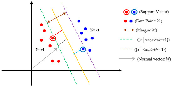
Figure 1. Optimized hyperplane for two-dimensional space (Linear-SVM) [23]. SVM: support vector machine.

According to Figure 1, $x_1$ is the data points of the two classes labeled $y_1=\left\{1,-1\right\}$ such that $⟨w, x⟩+b=0$ is the optimal hyperplane assigned in the middle of the other two lines, i.e., $\left\{x|⟨w, x⟩+b=+1\right\}$ and $\left\{x|⟨w, x⟩+b=-1\right\}$, so that w is a normal vector for the optimal hyperplane, and also, b represents the offset between the hyperplane and the origin plane. Furthermore, margin $M=2/w$ of the separator is the distance between support vectors. As a result, the maximum margin can be expressed in the form of the following constraint optimization equation [18,22,23,24]:

$$\mathrm{Minimize}:\frac{1}{2}{\left|w\right|}^2\mathrm{subjected}\mathrm{to}:y_i\left(w.x+b\right)-1\ge 0, \forall i.$$

(2)

To solve the optimization problem, the simplest way is to turn it into a dual problem. To obtain the dual form of the problem, the positive Lagrangian coefficients are multiplied by ${\alpha }_i\ge 0$ and subtracted from the objective function, resulting in the following equation called a primal problem (Lagrange’s initial equation, $L_p$) [18,23,24]:

$$L_p=\frac{1}{2}{\left|w\right|}^2-{\displaystyle \sum }_i{\alpha }_i(y_i\left(w.x+b\right))-1.$$

(3)

To solve the above equation, we need to apply the KKT conditions, which perform an important role in constraint optimization problems [18]. These conditions express the necessary and sufficient conditions for optimal response to constraint equations and must be a derivative of the function concerning the variables equal to zero. By applying KKT conditions to $L_p$ and if it is derived from w and b and set to zero, we will have [19,23,24]:

$$\frac{\partial }{\partial w_v}{L}_p=w_v-{\displaystyle \sum _i{\alpha }_i}{y}_i{x}_{iv}=0,v=1,\dots ,d.$$

(4)

$$\frac{\partial }{\partial b}{L}_p=-{\displaystyle \sum _i{\alpha }_i}{y}_i=0.$$

(5)

$${\alpha }_i\left(y_i\left(w.x+b\right)\right)-1\ge 0, i=1,\dots ,l, {\alpha }_i\ge 0, \forall i.$$

(6)

$${\alpha }_i\left(y_i\left(w.x+b\right)\right)-1\ge 0, \forall i.$$

(7)

With placement in Equation (3), we will have [19]:

$$Maximize:L_D={\displaystyle \sum _i{\alpha }_i}-\frac{1}{2}{\displaystyle \sum _i{\displaystyle \sum _j{\alpha }_i{\alpha }_j{y}_i{y}_j}}(x_i.x_j).$$

(8)

Equation (8) is called the dual problem. $L_p$ and $L_D$ are both computed from the same condition, so the optimal problem can be solved by computing the minimum $L_p$ or the maximum $L_p$, which is the $L_p$ double (with the condition ${\alpha }_1>=0$.

3.1.2. Nonlinear SVM

While data are not easily separated, a linear separator cannot be effective. However, if we transmit the data in a space with more dimensions, a solution can be found to separate them [18,22]. In the state mentioned in the previous section (Linear SVM), in fact, the inner product of the input training data in the support vectors of Equation (8) is used to form a linear separator in the form of a hyperplane. However, in the nonlinear state, we first map the data to a feature space or Hilbert H space with higher dimensions and then use the inner product of the obtained elements and linearly separate them. Figure 2 illustrates the above problem.

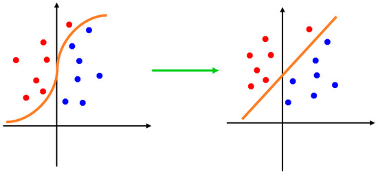
Figure 2. Nonlinear SVM [22].

Here, we assume: $\varphi :R^p\to H;x_i\to \varphi (x_i)$

Challenges transforming data to Hilbert space is as follows:

(1)

Performing computation in the feature space “Hilbert″ can be costly because it has more dimensions.

(2)

In general, the dimensions of this space are infinite, so working with this space is difficult.

(3)

In addition to the problem of increasing the computational cost, the generalization problem may also occur from very high dimensional spaces when analyzing and organizing data.

To overcome the feature space problem, a kernel trick is used. Therefore, in the learning algorithm, we use a kernel function $k\left(x_i,x_j\right)$ instead of the inner product $<\varphi (x_i),\varphi (x_j)>$ in the Hilbert H space. It has been shown in [21] with this indirect mapping that if the kernel function has Mercer’s condition, the kernel used is suitable, and the inseparable data in the mapped space will be separable, so replacing the kernel can generate a nonlinear algorithm from the linear algorithm mentioned. The kernel function $k\left(x_i,x_j\right)$ is as follows [18,23]:

$$k(x_i,x_j)={(1+x_i.x_j)}^d,$$

(9)

where d represents the dimension. So, to create a nonlinear SVM, we need to find a nonlinear separator hyperplane providing a solution as follows [18]:

$$\begin{array}{l}Maximize:\\ w(\alpha )={\displaystyle \sum _i^l{\alpha }_i}-\frac{1}{2}{\displaystyle \sum _{i=1}^l{\displaystyle \sum _{j=1}^l{\alpha }_i{\alpha }_j}}{y}_i{y}_{j}k(x_i,x_j),\end{array}$$

(10)

where ${\alpha }_i$ and ${\alpha }_j$ are positive Lagrangian coefficients. With this condition [18]

$${\displaystyle \sum _{i=1}^l{y}_i}{\alpha }_i=0,0\le {\alpha }_i\le c,i=1,\dots ,l,$$

(11)

“c” is a penalty factor or an additional cost for training faults, so that the “c” value is randomly selected by the user. A large “c” value means more penalties for faults. Finally, the decision function or separator function for the nonlinear SVM is as follows [18,22]:

$$f(x_i)=sign(<w,x_i>+b)={\displaystyle \sum _{i\in \mathrm{SV}}{\alpha }_i{y}_{i}k(x_i},x),$$

(12)

where SV are the support vectors. In this study, the radial basis function (RBF) [23,25] is selected as the kernel function, as shown below:

$$k(x_i,x_j)=\exp (-{\frac{\Vert x_i-x_j\Vert }{2{\sigma }^2}}^2)=\exp (-\gamma {\Vert x_i-x_j\Vert }^2),$$

(13)

where $\sigma$ is the base radius of the kernel function. In addition, the kernel parameter is $\gamma$. The value of the kernel parameter affects the training speed and the test speed so that this parameter is randomly selected as the base radius of the kernel function “$\sigma$” and the penalty factor “c”. It should be noted that the performance of SVM in terms of the accuracy of fault detection and generalization power severely depends on the state of the penalty factor “c” and the kernel parameter “$\gamma$”.

3.2. One-Class SVM

In one-class SVM or one SVM classification, the problem is to determine one class or one of the data from the rest of the feature space. In many applications, it is crucial that one of the classes is determined. Meanwhile, for the other class, no measurement is available [19]. It should be noted that the purpose of this study is to use a class of data to detect fault nodes.

Therefore, in this classification, it is assumed that we only have instances of one class called the target class, and all the other possible data, as well as outlier data, are distributed uniformly on the sides the target class. This one SVM classification problem is often unraveled by computing the target density or by a fit model for the SVM classifier.

According to the theory of Scholkopf et al. [26,27], it is presumed that there exist some data sets with a probability distribution “P”, and we want to estimate a “simple” subset of the input space, so that the probability of a test point of “P” assigned outside the set “S” is equal to a predetermined value between 0 and 1. Therefore, they proposed a one-class classification method for solving the problem, trying to determine the decision function “F” which is positive on set “S” and negative on complement “S”. The functional form “F” is given by creating a kernel function for a small subset of the training data points.

Assuming the training data $x_1,x_2,\dots ,x_n\in R^n$, let “n” be the number of data points. There is also a mapping “$\varphi$” of a feature map $R^n\to f$, such as a map to the point product space, so that the result of the point product $<\varphi (x_i),\varphi (x_j)>$ in the image can be obtained by evaluating the kernel function according to Equation (13).

In fact, in the one-class classification method of the SVM model, the origin is the only member of the class assigned second, after transformation of the training data through a feature map “$\varphi$”. Then, using the kernel parameters “$\gamma$” and the penalty factor “c”, the target class is separated from the origin with the highest margin. The one SVM algorithm returns a decision function “F” that gives the “+1” value in a region with the most data points; otherwise, “−1”.

For a new point “$x_i$”, the value of the decision function “f(x)” is obtained by evaluating which side of the hyperplane is assigned to it in the feature space. To separate the dataset from the origin, we solve the following convex programming equation [19]:

$$\underset{w,b,{\xi }_i}{Minimize}:\frac{1}{2}{\Vert w\Vert }^2+c{\displaystyle \sum _{i=1}^n{\xi }_i}+b$$

(14)

with the constraint that: $⟨w.\varphi (x_i)⟩+b\ge 0-{\xi }_i,$ ${\xi }_i\ge 0,$ $i=1,\dots ,n$, where “ξ_i” is a positive slack variable that is defined in the problem constraints. Given the weight vector “w” and the width of the origin “b” to solve the problem in Equation (14), the decision function or separator function is obtained as follows [19]:

$$f\left(x\right)=sign\left(⟨w.\varphi \left(x\right)⟩+b\right)$$

(15)

Using the Lagrange theorem, we can obtain the dual problem of Equation (14) as follows [19]

$$\underset{{\alpha }_i}{Minimize}:\frac{1}{2}{\displaystyle \sum _{i=1}^n{\displaystyle \sum _{j=1}^n{\alpha }_i}}{\alpha }_{j}k(x_i,x_j)$$

(16)

with the constraint that:

$$i=1,\dots , n, 0\le {\alpha }_i\le c, {\displaystyle \sum }_i{\alpha }_i=1.$$

Whether the value of the penalty “c” is large or small, this random parameter is a constant value during the one SVM learning process. That is, all training data are performed equally during one SVM learning process. So, it leads to a higher sensitivity to faults related to points. In addition, the decision function “$f\left(x\right)$” for a one-class SVM is a “+1” or “−1” value, meaning that each data point is divided into two groups: the membership and non-membership of the relating class. There is a clear and unambiguous distinction between members and non-members of a set. Although, when modeling a system in which human determination is influenced, we observe this set as an inaccurate separation line. The decision function should be generalized so that the values allocated to the penalty and kernel random parameters are determined within a specific range and the degree of membership of these parameters is indicated in the set.

3.3. Fuzzy One-Class SVM

In some applications, the effects of training data on the learning model are different. In these applications, it is observed that some points are more important than others in the classification model. We need the more crucial and valuable points to be properly classified and some training points such as noises, whether they are incorrectly classified or not, to not pay attention. This means that each training point can not exactly belong to one of the two classes. The majority of these points (90%) may belong to a class and 10% may be worthless, or 20% may belong to a class and 80% may be worthless.

As previously mentioned, one of the major challenges of an SVM is the lack of ability to separate accurate data points or safe nodes from faulty nodes [18,19]. In fact, SVM cannot discard faulty nodes. One solution is to consider fuzzy membership $0<{\mu }_i\le 1$ for each training point “$x_i$”. This fuzzy membership of “${\mu }_i$” can be considered as the status of the training point of a class in the classification problem, and the value ($1-{\mu }_i$) can be considered as a meaningless status. As a result, the same behavior across all data points may lead to inadequate compatibility with SVM. Hence, the fuzzy one SVM method assigns each data point to a membership value due to its proportional importance in the class and the behavior of the training data points with varying measurements of importance in the learning process [19]. We assume to have a set of training data points with the relating fuzzy membership: $(x_1,{\mu }_1),\dots ,(x_n,{\mu }_n)$.

Each training point $x_i\in R^n$ has a fuzzy membership of $0<{\mu }_i\le 1.$ Since the fuzzy membership “${\mu }_i$” is the point state of “x_i” relative to the target class and parameter “ξ_i” is a fault rate in one-class SVM, the expression “${\mu }_i {\xi }_i$” is the fault rate with various weighting. Then, the optimization problem based on a constraint for the fuzzy one SVM is demonstrated as follows [19]

$$\underset{w,b,{\xi }_i}{Minimize}:\frac{1}{2}{\Vert w\Vert }^2+c{\displaystyle \sum _{i=1}^n\mu {\xi }_i}+b$$

(17)

with the constraint that:

$$⟨w.\varphi (x_i)⟩+b\ge 0-{\xi }_i,{\xi }_i\ge 0,i=1,\dots ,n.$$

We can solve this optimization problem by Equation (17) in the dual variable by determining the point at which the bivariate function has partial derivatives equal to zero. However, in it, the function has neither the maximum nor the least value for the Lagrangian equation. Then, we can find out according to the following Lagrangian equation [19]:

$$L=\frac{1}{2}{\Vert w\Vert }^2+c{\displaystyle \sum _{i=1}^n\mu {\xi }_i}+b-{\displaystyle \sum _{i=1}^n{\alpha }_i}(⟨w.\varphi (x_i)⟩+b+{\xi }_i)-{\displaystyle \sum _{i=1}^n{\beta }_i{\xi }_i},$$

(18)

where “${\alpha }_i$” and “${\beta }_i$” are positive Lagrangian coefficients. By deriving “L” with “w, b” and “ξ_i” equal to zero assigns, the result is obtained as follows [19]:

$$\frac{\partial l}{\partial w}=w-{\displaystyle \sum _{i=1}^n{\alpha }_i}\varphi (x_i)=0\Rightarrow w={\displaystyle \sum _{i=1}^n{\alpha }_i}\varphi (x_i),$$

(19)

$$\frac{\partial l}{\partial b}=1-{\displaystyle \sum _{i=1}^n{\alpha }_i}=0\Rightarrow {\displaystyle \sum _{i=1}^n{\alpha }_i}=1,$$

(20)

$$\frac{\partial l}{\partial {\xi }_i}=c{\mu }_i-{\alpha }_i-{\beta }_i=0\Rightarrow {\alpha }_i=c{\mu }_i-{\beta }_i,{\alpha }_i\le c{\mu }_i.$$

(21)

By replacing Equations (19)–(21) in the Lagrange equation, the dual problem is obtained as follows [19]

$$\underset{{\alpha }_i}{Minimize}:\frac{1}{2}{\displaystyle \sum _{i=1}^n{\displaystyle \sum _{j=1}^n{\alpha }_i}}{\alpha }_{j}k(x_i,x_j)$$

(22)

with the constraint that:

$$0\le {\alpha }_i\le c{\mu }_i,i=1,\dots ,n,{\displaystyle \sum _i{\alpha }_i}=1.$$

Considering the above equation, it should be addressed that the only difference between the fuzzy one SVM and the initial one-class model is the upper boundary of the “${\alpha }_i$” Lagrangian coefficient for each training point, in which “$x_i$” means “$c{\mu }_i$”. The fuzzy decision function is also as follows [19]:

$$f(x_i)=sign(<w,x_i>+b)={\displaystyle \sum _{i\in \mathrm{SV}}{\alpha }_i{y}_{i}k(x_i},x).$$

(23)

For “$y_i$”, consider the fuzzy membership of $0<{\mu }_i\le 1$.

For the proposed method in this study, the fuzzy decision function is as follows:

$$f\left(x_i\right)=sign\left(⟨w, x_i⟩+b\right)= \{\begin{array}{c}Yes \left(safe node\right), if y_i=1-{\mu }_i\\ No \left(Fault node\right), if y_i=-{\mu }_i\end{array}.$$

(24)

3.4. MB-FLEACH Algorithm

The proposed MB-FLEACH algorithm in [4] is a new way to select a super cluster head (SCH) in WSNs, as this SCH is the node that creates optimal energy consumption in the network, and this procedure leads to an increase of the network lifetime. This algorithm, in terms of energy consumption and network lifetime has the best performance with the constraint of the mobility of the base station compared with the other algorithms in a distributed system with two defined scenarios. The MB-FLEACH algorithm is shown in Figure 3.

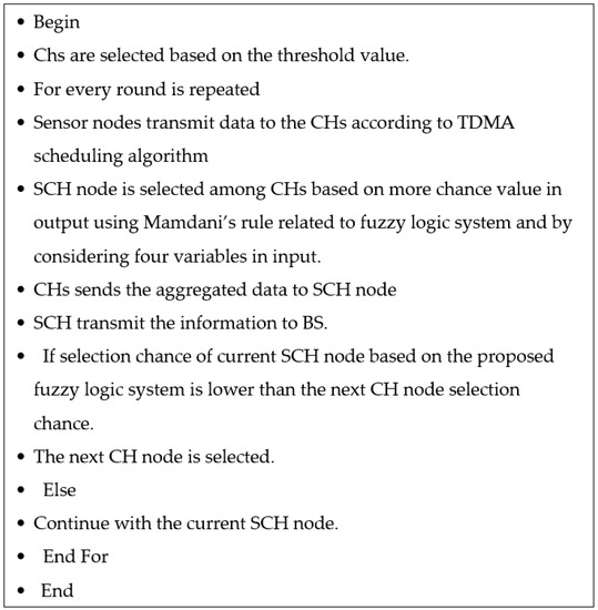
Figure 3. MB-FLEACH algorithm [4].

Using the MB-FLEACH algorithm in scenarios defined for sensor nodes in a distributed wireless network across all rounds has the least energy consumption. It should be noted that for this algorithm, the detection of fault nodes has not been performed. In this study, we apply the fuzzy one SVM algorithm to the MB-FLEACH algorithm of the fault node detection in the network.

3.5. The Proposed Method

As mentioned in the preceding section, the MB-FLEACH algorithm is suitable for selecting an SCH to reduce the energy consumption for a distributed system. Hence, in this study, we decide to apply the MB-FLEACH algorithm to a proposed method called the FCS-MBFLEACH of the fault detection to compute the fault detection rate by analyzing the nodes in the network. We will observe that this approach will have a very crucial impact on the early detection of the fault, as it reduces energy consumption compared to the MB-FLEACH, one SVM, and fuzzy one SVM methods. As a result, with this method, the network lifetime will be increased. The proposed algorithm of SCS-MBFLEACH is illustrated in Figure 4.

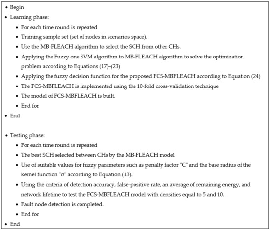
Figure 4. The proposed FCS-MBFLEACH algorithm.

4. Experiments

In this section, first, fault detection algorithms such as one SVM, fuzzy one SVM, and the fuzzy one SVM by applying the MB-FLEACH algorithm, namely FCS-MBFLEACH, are evaluated in terms of criteria regarding the accuracy of fault detection, false-positive rate (FPR), the average remaining energy, and network lifetime. These scenarios are described below:

(1)

The first scenario: The nodes are randomly distributed with 50 sensor nodes in a 100 square meter region so that the base station location changes randomly. It is given that the base station’s initial location is assigned in the 30 m × 30 m coordinate.

(2)

The second scenario: In this scenario, the density of the node changes. It is given that 100 nodes are randomly distributed in the same first scenario space so that the probability of the base station arriving at the next location is randomly determined based on the appropriate location of the base station with respect to the selected SCH.

The network parameters are the same as those in Table [4], as shown in Table 1.

Table 1. Network parameters.

Parameter Values
Platform	Windows 10
Tool used	Opnet vs. 14.5
Network size	100 m × 100 m
Maximum number of rounds	800
Base station location	30 m × 30 m
Mobility of base station	Random
Node distribution	Random
Energy startup	1 J
Ɛfs	15 pJ/bit/m2
Ɛmp	0.0015 pJ/bit/m4
Eelec	60 nJ/bit
EDA	5 nJ/bit/signal
Data packet size	500 bytes
Threshold distance (d0)	65 m

The proposed solution for fault detection in the wireless sensor network consists of two phases: one is used to train the models, which we call the learning phase, while the other phase is called the testing phase, which is used to test the models.

4.1. Learning Phase

In this study, we carry out the defined scenarios so that the set of training samples is the same as the number of randomly located sensor nodes in the network space. In this phase, the classification of models is based on learning data points as sensor nodes. This method allows us to use expert knowledge in decision making. In this phase, data is the most important element in the fault node detection process in WSNs.

As stated, these data are the same sensor nodes that the proposed method model FCS-MBFLEACH should build in the learning phase. Therefore, the suitable SCH between CHs should first be generated by the MB-FLEACH algorithm [4]. Then, the proposed model for the MB-FLEACH algorithm is applied to the FCS paradigm. The nodes in the network can play a crucial role as the cluster heads as well as the suitable supercluster head for solving problems that appear as faults in wireless sensor networks. Finally, the learning stage of the sensor nodes in the distributed network is completed as shown in Figure 5.

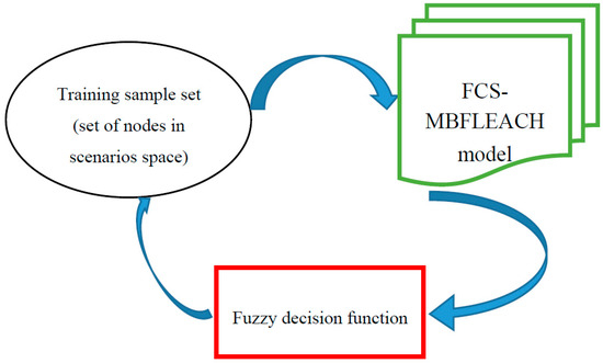
Figure 5. The learning phase.

In this phase, the propose is to create a fuzzy decision function that can be used at different time rounds to classify any new sensor nodes in the network as faults by the fault detection model. The solution of learning data as a node in the proposed method is based on the statistical learning technique. Then, the fuzzy decision function created according to Equation (24) in the super cluster head will be applied to classify the nodes. The set of sensor nodes is used as the learning dataset according to the defined scenario. The learning phase was implemented using the 10-fold cross-validation technique. It should be noted that the sensor nodes are initially randomly distributed as a set of normal nodes in the network.

4.2. Testing Phase

We used Opnet modeler simulator vs. 14.5 to test and evaluate the proposed method and other classification methods including one SVM, fuzzy one SVM, and MB-FLEACH. These models, which were all trained in the learning phase set, can be compared in the test set. Considering the performance of the proposed method in the test set, we try to deduce suitable values of fuzzy parameters including the penalty factor “c” and kernel parameter “$\gamma$”. It should be noted that in the testing phase, the nodes are tested. In fact, nodes are tested to estimate the accuracy of fault detection. Initially, the best SCH is selected between different CHs by the MB-FLEACH algorithm. Then, the proposed FCS-MBFLECH model is applied to detect the fault sensor node in the set of nodes relating to the SCH according to the fuzzy decision function. Regarding the test phase, the fault detection process as a comprehensive detection system is shown in Figure 6.

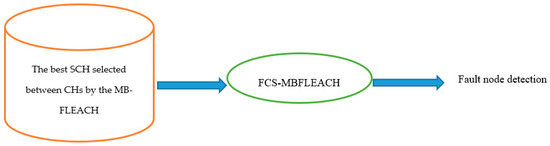
Figure 6. Fault detection system.

5. Results

As we mentioned in the previous section, from the scenario defined in this study, the nodes are randomly distributed in the regions. A 10-fold cross-validation technique was used to evaluate the performance of the proposed method to obtain the average detection accuracy for the methods. The simulation results were performed using Opnet software for the desired models. For each scenario, simulations were performed on average for 40 minutes 10 times so that at each time pried for each scenario, the fault node detection was based on the fault detection system. It should be noted that for each scenario, we set values of “1.0” and “0.5” for the kernel function parameters based on Equation (13), such as the penalty factor “c” and base radius “$\sigma$”, respectively. So, the value of “$\gamma$” should be optimized. Finally, to evaluate the proposed FCS-MBFLEACH method, this method was compared with fault detection methods such as one SVM, fuzzy one SVM, and MB-FLEACH. Two criteria were used to evaluate the fault node detection by comparing these methods. These criteria include the detection accuracy (DA) and the false-positive rate (FPR) described below and in the following subsections.

Given that after fault detection for the sensor nodes in the network, other criteria such as the remaining energy consumption and network lifetime were examined to observe which of the methods with the measure of diagnosis made have the least energy consumption and the highest network lifetime.

In the proposed FCS-MBFLEACH method, we first have the number of cluster heads created by the MB-FLEACH algorithm so that the suitable supercluster head is selected between the cluster heads [4].

5.1. Fault Detection Accuracy

Detection accuracy (DA) [5] refers to the number of correctly detected faulty nodes to the total number of actual fault nodes, and it is given below:

$$\mathrm{DA}=\frac{\mathrm{number}\mathrm{of}\mathrm{correctly}\mathrm{detected}\mathrm{faulty}\mathrm{nodes}}{\mathrm{total}\mathrm{number}\mathrm{of}\mathrm{actual}\mathrm{faulty}\mathrm{nodes}}.$$

(25)

Based on the average of fault detection accuracy, the fault node detection methods were compared according to the defined scenarios. The crucial note about this criterion is that if the fault detection is correctly and quickly performed with high accuracy, the least energy is consumed for the node in the network. As a result, it increases the lifetime of the network. Detection accuracy criteria were also computed based on densities of five and 10 for sensor nodes in rounds 1, 57, 112, 342, 678, and 800. The fault detection accuracy is computed for the two scenarios.

5.1.1. Fault Detection Accuracy for the First Scenario

The average of fault detection accuracy against the probability of sensor node fault for the first scenario with densities equal to 5 and 10 is shown in Figure 7 and Figure 8. Based on these figures, it can be concluded that a common feature among the methods is that with the increasing probability of sensor node fault, the average of the accuracy of detection decreases.

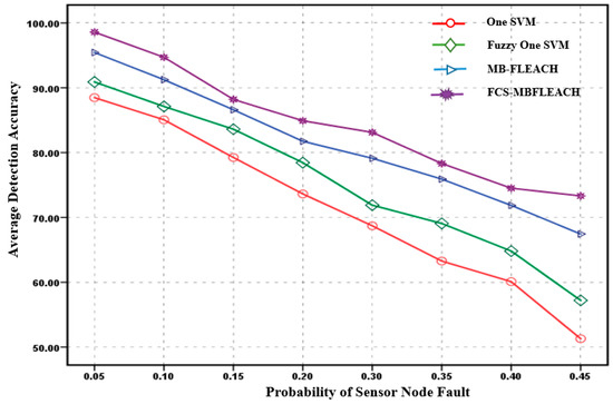
Figure 7. Average detection accuracy of sensor node faults with a density equal to five for the first scenario.

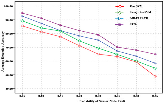
Figure 8. Average detection accuracy of sensor node faults with a density equal to 10 for the first scenario.

According to Figure 7, the proposed FCS-MBFLEACH method at different time points has the highest detection accuracy compared to other methods. When the probability of fault is equal to 5%, the average fault detection accuracy for the proposed FCS-MBFLEACH method compared with one SVM, fuzzy one SVM, and MB-FLEACH is improved 10.11%, 7.69%, and 3.15%, respectively. In addition, for the highest probability of fault (45%), the detection accuracy of the proposed method compared to one SVM, fuzzy one SVM, and MB-FLEACH has preference with the values of 22.03%, 16.12%, and 5.88%, respectively.

In Figure 8, the accuracy of node fault detection in the network for the mentioned methods in different scheduling is computed. The accuracy of the proposed FCS-MBFLEACH detection method for the 5% fault probability compared to the one SVM, fuzzy one SVM, and MB-FLEACH methods was improved, with values of 9.30%, 5.61%, and 2.17%, respectively. In addition, for the highest fault probability of 45%, the detection accuracy of the proposed method was improved by 16.07%, 10.16%, and 6.55% for one SVM, fuzzy one SVM, and MB-FLEACH, respectively.

5.1.2. Fault Detection Accuracy for the Second Scenario

The average fault detection accuracy against the probability of the fault node for the second scenario with densities of five and 10 is shown in Figure 9 and Figure 10.

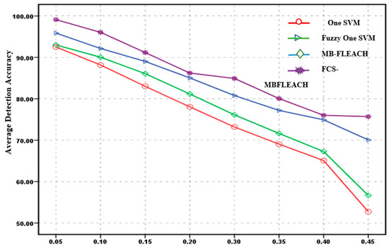
Figure 9. Average detection accuracy of sensor node faults with a density equal to five for the second scenario.

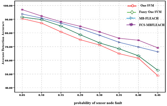
Figure 10. Average detection accuracy of sensor node faults with a density equal to 10 for the second scenario.

Considering Figure 9, the accuracy of fault detection for the methods with the 5% fault probability is computed. Hence, the accuracy of the FCS-MBFLEACH method compared to one SVM, fuzzy one SVM, and MB-FLEACH methods was improved by 7.60%, 6.45%, and 3.12%, respectively. So, for the highest probability of 45%, the detection accuracy of the proposed method was improved by 22.95%, 19.04%, and 5.63% for one SVM, fuzzy one SVM, and MB-FLEACH, respectively. For Figure 10, the accuracy of fault detection with the 5% fault probability is computed so that the accuracy of the FCS-MBFLEACH method was denoted with this method compared to the one SVM, fuzzy one SVM, and MB-FLEACH methods, which was improved by 6.59%, 5.43%, 3.19%, respectively. In addition, for the highest probability of 45%, the average accuracy of the proposed method compared with the other methods such as one SVM, fuzzy one SVM, and MB-FLEACH was improved by 20.33%, 16.39%, and 2.89%, respectively.

5.2. False-Positive Rate

The false-positive rate (FPR) is one of the crucial criteria for detecting node faults in WSN [5]; it is also called the false alarm rate. This criterion is defined as the ratio of the number of safe nodes detected as a fault to the total number of sensor nodes faults, which is as follows:

$$\mathrm{FPR}=\frac{\mathrm{Number}\mathrm{of}\mathrm{safe}\mathrm{nodes}\mathrm{detected}\mathrm{as}\mathrm{a}\mathrm{fault}}{\mathrm{Total}\mathrm{number}\mathrm{of}\mathrm{fault}\mathrm{nodes}}.$$

(26)

The FPR criterion has been examined based on different rounds for the one SVM, fuzzy one SVM, MB-FLEACH, and FCS-MBFLEACH methods in both scenarios with five and 10 node densities.

5.2.1. False-Positive Rate for the First Scenario

The average false-positive rate criterion against the probability of sensor node faults for the first scenario with densities of five and 10 is shown in Figure 11 and Figure 12. Given these figures, in both scenarios, the performance of each algorithm can be observed in rounds defined by node densities of five and 10, so that one common feature among the methods is that the increasing probability of sensor node fault in the network increases the average FPR. Clearly, in both scenarios with different densities, the FPR for the proposed method is lower than those of the other methods.

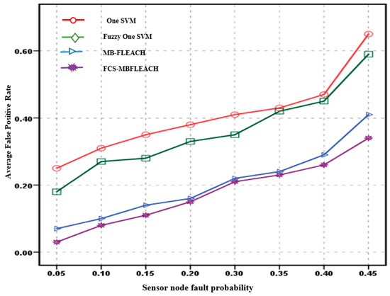
Figure 11. Average false positive rate for sensor node faults with a density equal to five for the first scenario.

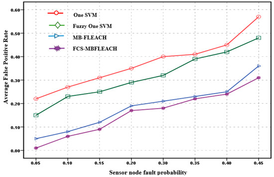
Figure 12. The average false positive rate for sensor node faults with a density equal to 10 for the first scenario.

According to Figure 11, in the first scenario for the proposed method with a 5% fault probability, the false positive rate is 3%. In contrast, the false positive rates for one SVM, fuzzy one SVM, and MB-FLEACH were 25%, 18%, and 7%, respectively. This criterion is also 34% for the proposed method with a 45% probability of fault compared with 65%, 59%, and 41% for one SVM, fuzzy one SVM, and MB-FLEACH, respectively.

Thus, according to Figure 12, for the proposed method with a 5% fault probability, the average false positive rate is 1%. While the average false positive rates for one SVM, fuzzy one SVM, and MB-FLEACH methods are 22%, 15%, and 5%, respectively. In addition, this criterion for the proposed method is 31% with a 45% probability of fault, which is 57%, 48%, and 36% higher than those for one SVM, fuzzy one SVM, and MB-FLEACH, respectively.

5.2.2. False-Positive Rate for the Second Scenario

The false-positive rate against the probability of fault sensor nodes for the second scenario is shown in Figure 13 and Figure 14.

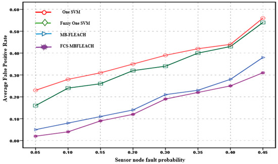
Figure 13. Average false positive rate for sensor node faults with a density equal to 5 for the second scenario.

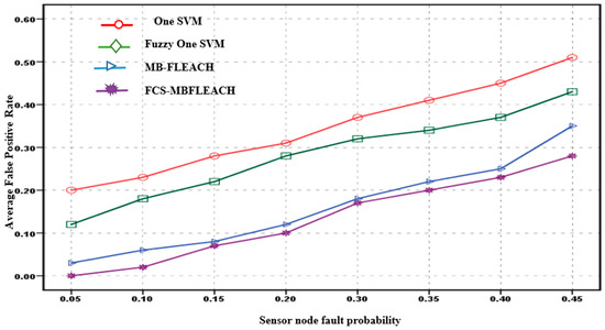
Figure 14. Average false positive rate for sensor node faults with a density equal to 10 for the second scenario.

According to Figure 13, in the second scenario for the proposed method with a 5% fault probability, the false positive rate is 2%. Meanwhile, the false positive rates for one SVM, fuzzy one SVM, and MB-FLEACH are 23%, 16%, and 5%, respectively. In addition, the false positive rate for the proposed method is 45% with a 31% probability of fault compared with those of one SVM, fuzzy one SVM, and MB-FLEACH, which were computed as 56%, 54%, and 38%, respectively.

Thus, according to Figure 14, for the proposed FCS-MBFLEACH method with a 5% fault probability, the false positive rate is null. Meanwhile, the false positive rates for one SVM, the fuzzy one SVM, and MB-FLEACH methods are 20%, 12% and 3%, respectively. In addition, the false positive rate for the proposed method with a 45% probability of fault is 28%, which is 51%, 43%, and 35% higher than those for one SVM, fuzzy one SVM, and MB-FLEACH, respectively.

5.3. Average Remaining Energy

The average remaining energy after detecting the sensor node fault in the network regarding the cluster heads is crucial for selecting the super cluster head for the proposed FCS-MBFLEACH method so that in both scenarios, the average of remaining energy in joules against different rounds after the fault detection for the methods is computed, as shown in Figure 15 and Figure 16. The values of the average remaining energy for the algorithms are assigned for two scenarios in Table 2 and Table 3.

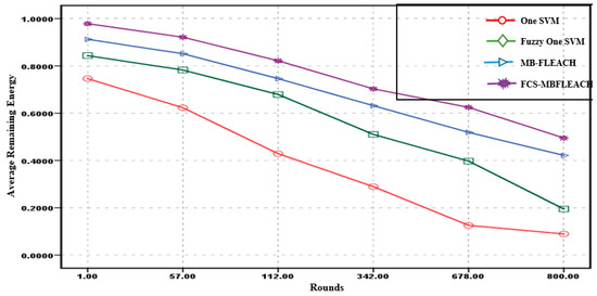
Figure 15. Average remaining energy for fault detection methods in different rounds for the first scenario.

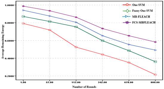
Figure 16. Average remaining energy for fault detection methods in different rounds for the second scenario.

Table 2. Average remaining energy in different rounds for the first scenario.

Algorithms	Average Remaining Energy
	Scenario 1
	Round 1	Round 57	Round 112	Round 342	Round 678	Round 800
One SVM	0.7463	0.6231	0.4289	0.2893	0.1257	0.0893
Fuzzy one SVM	0.8435	0.7825	0.6791	0.5102	0.3974	0.1948
MB-FLEACH	0.9125	0.8516	0.7462	0.6318	0.5189	0.4215
FCS-MBFLEACH	0.9786	0.9215	0.8217	0.7029	0.6248	0.4951

Table 3. Average remaining energy in different rounds for the second scenario.

Algorithms	Average Remaining Energy
	Scenario 2
	Round 1	Round 57	Round 112	Round 342	Round 678	Round 800
One SVM	0.7921	0.7184	0.5249	0.4421	0.3514	0.2143
Fuzzy one SVM	0.8714	0.8146	0.7536	0.5978	0.4852	0.3610
MB-FLEACH	0.9412	0.8761	0.8053	0.6538	0.5549	0.4914
FCS-MBFLEACH	0.9873	0.9352	0.8624	0.7348	0.6534	0.5827

Based on Table 2 and Table 3 as well as Figure 15 and Figure 16, it can be observed, on average, that the remaining energy for the proposed FCS-MBFLEACH method is more than those of the other methods for all the rounds in the network.

5.4. Network Lifetime

There is a concept of stability time in a wireless sensor network i.e., network lifetime, which refers to the time between the death of the first node or FND to the death of half the nodes or HND; this is called the lifetime of the network [4]. In addition, another concept that we will discuss later is called half node alive, which has been much discussed and researched. The value of half node alive is equal to the period in which half of the network nodes die. The results of the simulation show that the proposed FCS-MFLEACH method has better performance than the other algorithms in terms of FND and HND criteria. The first node deaths and half node deaths for all the methods are shown in Figure 17 and Figure 18 in both scenarios.

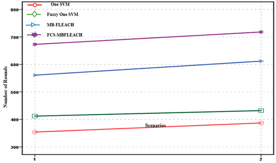
Figure 17. First node death (FND) for all methods in two scenarios.

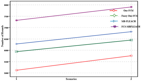
Figure 18. Half node death (HND) for all methods in two scenarios.

5.5. Network Lifetime for the First Scenario

In the simulation performed, it was observed that the network lifetime based on first node death criterion in Figure 17 illustrates a better performance in both scenarios for the proposed FCS-MBFLEACH method than the other methods, as the first node death occurs for the first scenario of the proposed method in round 673, and it occurs for the second scenario in round 718. The FND and HND criteria considered in this study are described in Table 4.

Table 4. A comparison between the proposed algorithms in terms of remaining energy, as well as FND and HND criteria.

Algorithms	FND		HND
	Scenario 1	Scenario 2	Scenario 1	Scenario 2
One SVM	354	387	512	576
Fuzzy one SVM	412	432	594	645
MB-FLEACH	561	612	628	682
FCS-MBFLEACH	673	718	732	791

In addition, the network lifetime based on HND in Figure 18 shows better performance in both scenarios for the proposed FCS-MBFLEACH method compared to the other methods. As for the proposed method, HND will occur for the first scenario in round 732, and it will occur for the second scenario in round 791. Finally, a comparison between the SVM, fuzzy one SVM, MB-FLEACH, and FCS-MBFLEACH algorithms in terms of accuracy detection and FPR criteria is demonstrated for two scenarios with densities equal to 5 and 10 in Table 5.

Table 5. A comparison between the proposed algorithms in terms of detection accuracy and FPR criteria.

Algorithms	Detection Accuracy (%) with Density Equal to 5				FPR with Density Equal to 5				Detection Accuracy (%) with Density Equal to 10				FPR with Density Equal to 10
	Scenario 1 for Fault Probability		Scenario 2 for Fault Probability		Scenario 1 for Fault Probability		Scenario 2 for Fault Probability		Scenario 1 for Fault Probability		Scenario 2 for Fault Probability		Scenario 1 for Fault Probability		Scenario 2 for Fault Probability
	5	45	5	45	5	45	5	45	5	45	5	45	5	45	5	45
One SVM	88.48	51.29	92.51	52.74	0.25	0.65	0.23	0.56	85.51	48.84	90.42	48.75	0.22	0.57	0.20	0.51
Fuzzy one SVM	90.90	57.20	93.01	56.65	0.18	0.59	0.16	0.54	89.20	54.75	91.58	52.69	0.15	0.48	0.12	0.43
MB-FLEACH	95.44	67.44	95.87	70.06	0.07	0.41	0.05	0.38	92.64	58.36	93.82	66.19	0.05	0.36	0.03	0.35
FCS-MBFLEACH	98.59	73.32	99.12	75.69	0.03	0.34	0.02	0.31	94.81	64.91	97.01	69.08	0.01	0.31	0.00	0.28

Based on Table 5, it can be deducted that the proposed method of FCS-MBFLEACH outperforms the other classification methods in terms of detection accuracy and FPR criteria in both scenarios.

6. Conclusions and Future Work

In this paper, a machine learning classification method for computing the fault detection accuracy with an effective energy-aware approach in mobile wireless sensor networks is proposed called FCS-MBFLEACH. The investigated methods for fault detection including one SVM, fuzzy one SVM, MB-FLEACH, and FCS-MBFLEACH were performed based on the defined scenarios [4]. One of the problems with fault detection in WSNs is early fault detection so that we have the least energy consumption for sensor nodes, so we used the MB-FLEACH approach to achieve this purpose. We first used the MB-FLEACH algorithm to select the suitable SCH [4] with the most remaining energy, the least distance to the mobile base station, and the greatest centrality of the node. Then, this algorithm was applied to the fuzzy one SVM model based on the creation of the fuzzy decision function.

Finally, according to Table 2, Table 3, Table 4 and Table 5, by comparing the proposed FCS-MBFLEACH method with machine learning methods such as one SVM, fuzzy one SVM, and MB-FLEACH, we concluded that FCS-MBFLEACH has the best performance in terms of detection accuracy, false positive rate, average remaining energy, and network lifetime criteria.

In future work, we can use other algorithms in combination, including deep neural networks, the genetic evolutionary algorithm, as well as the particle swarm optimization algorithm with other scenarios and other datasets.

References

- Heinzelman, W.B.; Chandrakasan, A.P.; Balakrishnan, H. An application-specific protocol architecture for wireless micro sensor networks. IEEE Trans. Wirel. Commun. 2002, 1, 660–670. [Google Scholar] [CrossRef]
- Yick, J.; Mukherjee, B.; Ghosal, D. Wireless sensor network survey. Comput. Netw. 2008, 52, 2292–2330. [Google Scholar] [CrossRef]
- Katiyar, V.; Chand, N.; Soni, S. A Survey on Clustering Algorithms for Heterogeneous Wireless Sensor Networks. Int. J. Appl. Eng. Res. 2010, 1, 745–754. [Google Scholar]
- Hosseini, S.M.; Joloudari, J.H.; Saadatfar, H. MB-FLEACH: A New Algorithm for Super Cluster Head Selection for Wireless Sensor Networks. Int. J. Wirel. Inf. Netw. 2019, 26, 113–130. [Google Scholar] [CrossRef]
- Muhammed, T.; Shaikh, R. An analysis of fault detection strategies in wireless sensor networks. J. Netw. Comput. Appl. 2017, 78, 267–287. [Google Scholar] [CrossRef]
- Chen, J.; Kher, S.; Somani, A. Distributed fault detection of wireless sensor networks. In Proceedings of the 2006 Workshop on Dependability Issues in Wireless ad hoc Networks and Sensor Networks, Florence, Italy, 28 June–1 July 2006; pp. 65–72. [Google Scholar]
- Cheng, Y.; Liu, Q.; Wang, J.; Wan, S.; Umer, T. Distributed Fault Detection for Wireless Sensor Networks Based on Support Vector Regression. Wirel. Commun. Mob. Comput. 2018, 2018, 1–8. [Google Scholar] [CrossRef]
- Jiang, P. A new method for node fault detection in wireless sensor networks. Sensors 2009, 9, 1282–1294. [Google Scholar] [CrossRef]
- Kai, L.I.U.; Li, P.E.N.G. Research on fault diagnosis algorithm for clustering node in wireless sensor networks. Transducer Microsyst. Technol. 2011, 4, 312–336. [Google Scholar]
- Feng, Z.; Fu, J.Q.; Wang, Y. Weighted distributed fault detection for wireless sensor networks Based on the distance. In Proceedings of the 33rd Chinese Control Conference, Nanjing, China, 28–30 July 2014; pp. 322–326. [Google Scholar]
- Maronna, R.A.; Martin, R.D.; Yohai, V.J.; Salibián-Barrera, M. Robust Statistics; John Wiley Sons: Chichester, UK, 2006; pp. 978–990. [Google Scholar]
- Panda, M.; Khilar, P.M. Distributed self fault diagnosis algorithm for large scale wireless sensor networks using modified three sigma edit test. Ad Hoc Netw. 2015, 25, 170–184. [Google Scholar] [CrossRef]
- Xu, X.; Geng, W.; Yang, G.; Bessis, N.; Norrington, P. LEDFD: A low energy consumption distributed fault detection algorithm for wireless sensor networks. Int. J. Distrib. Sensor Netw. 2014, 10, 1–10. [Google Scholar] [CrossRef]
- Artail, H.; Ajami, A.; Saouma, T.; Charaf, M. A faulty node detection scheme for wireless sensor networks that use data aggregation for transport. Wirel. Commun. Mob. Comput. 2016, 16, 1956–1971. [Google Scholar] [CrossRef]
- Emadi, H.S.; Mazinani, S.M. A novel anomaly detection algorithm using DBSCAN and SVM in wireless sensor networks. Wirel. Pers. Commun. 2018, 98, 2025–2035. [Google Scholar] [CrossRef]
- Qiu, T.; Zhao, A.; Xia, F.; Si, W.; Wo, D.O. ROSE: Robustness strategy for scale-free wireless sensor networks. IEEE/ACM Trans. Netw. (TON) 2017, 25, 2944–2959. [Google Scholar] [CrossRef]
- Qiu, T.; Qiao, R.; Wu, D.O. EABS: An event-aware backpressure scheduling scheme for emergency Internet of Things. IEEE Trans. Mob. Comput. 2017, 20, 72–84. [Google Scholar] [CrossRef]
- Lin, C.F.; Wang, S.D. Fuzzy support vector machines. IEEE Trans. Neural Netw. 2002, 13, 464–471. [Google Scholar]
- Hao, P.Y. Fuzzy one-class support vector machines. Fuzzy Sets Syst. 2008, 158, 2317–2336. [Google Scholar] [CrossRef]
- Vapnik, V. Statistical Learning Theory; Wiley: Hoboken, NJ, USA, 1998; pp. 156–160. [Google Scholar]
- Vapnik, V. The Nature of Statistical Learning Theory; Springer Science Business Media: Medford, MA, USA, 2013. [Google Scholar]
- Zidi, S.; Moulahi, T.; Alaya, B. Fault detection in wireless sensor networks through SVM classifier. IEEE Sens. J. 2017, 18, 340–347. [Google Scholar] [CrossRef]
- Boser, B.E.; Guyon, I.M.; Vapnik, V.N. A training algorithm for optimal margin classifiers. In Proceedings of the 5th Annual ACM Workshop on Computational Learning Theory, Pittsburgh, PA, USA, 27–29 July 1992; pp. 144–152. [Google Scholar]
- Tax, D.M.J.; Duin, R.P.W. Support vector data description. Mach. Learn. 2004, 54, 45–66. [Google Scholar] [CrossRef]
- Zeng, N.; Qiu, H.; Wang, Z.; Liu, W.; Zhang, H.; Li, Y. A new switching-delayed-PSO-based optimized SVM algorithm for diagnosis of Alzheimer’s disease. Neurocomputing 2018, 320, 195–202. [Google Scholar] [CrossRef]
- Schölkopf, B.; Platt, J.C.; Shawe-Taylor, J.; Smola, A.J.; Williamson, R.C. Estimating the support of a high-dimensional distribution. Neural Comput. 2001, 13, 1443–1471. [Google Scholar] [CrossRef]
- Mansoor, K.; Ghani, A.; Chaudhry, S.A.; Shamshirband, S.; Ghayyur, S.A.K.; Mosavi, A. Securing IoT-Based RFID Systems: A Robust Authentication Protocol Using Symmetric Cryptography. Sensors 2019, 19, 4752. [Google Scholar] [CrossRef] [PubMed]
© 2019 by the authors. Licensee MDPI, Basel, Switzerland. This article is an open access article distributed under the terms and conditions of the Creative Commons Attribution (CC BY) license (http://creativecommons.org/licenses/by/4.0/).