An Efficient Conjugate Gradient Method for Convex Constrained Monotone Nonlinear Equations with Applications †


Abstract
1. Introduction
2. Algorithm: Motivation and Convergence Result
- ()
- The mapping F is monotone, that is,
- ()
- The mapping F is Lipschitz continuous, that is there exists a positive constant L such that
- ()
- The solution set of (1), denoted by , is nonempty.
| Algorithm 1: (DCG) |
| Step 0. Given an arbitrary initial point , parameters , , and set . Step 1. If , stop, otherwise go to Step 2. Step 2. Compute using Equation (4). Step 3. Compute the step size such that Step 4. Set . If and , stop. Else compute where Step 5. Let and go to Step 1. |
3. Numerical Examples
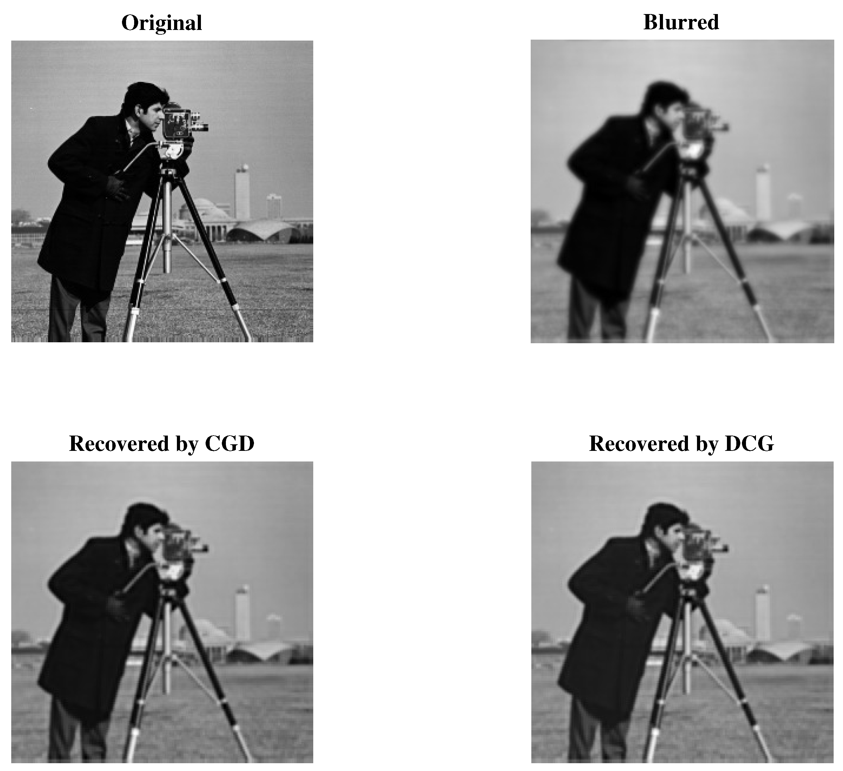
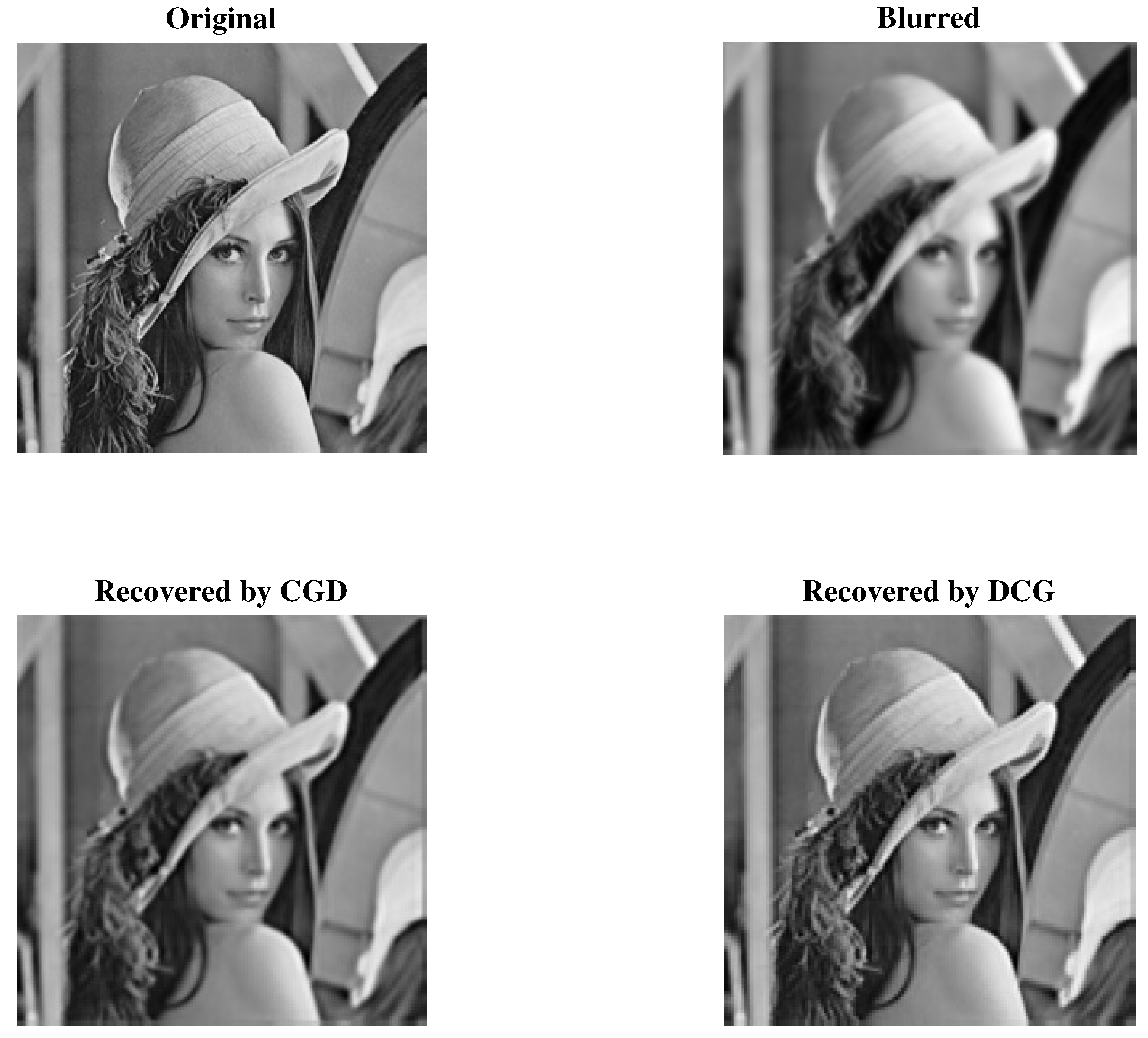
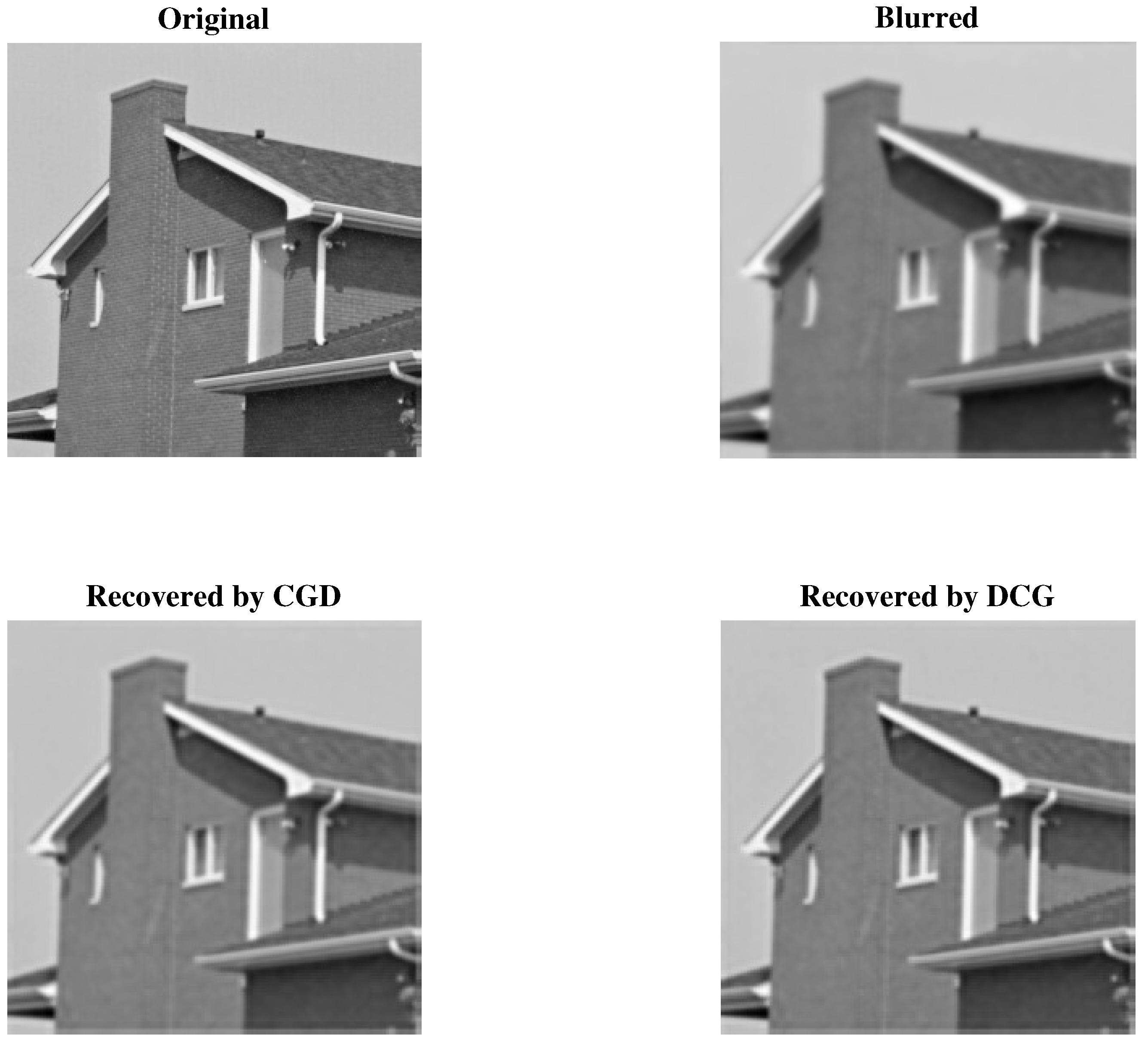
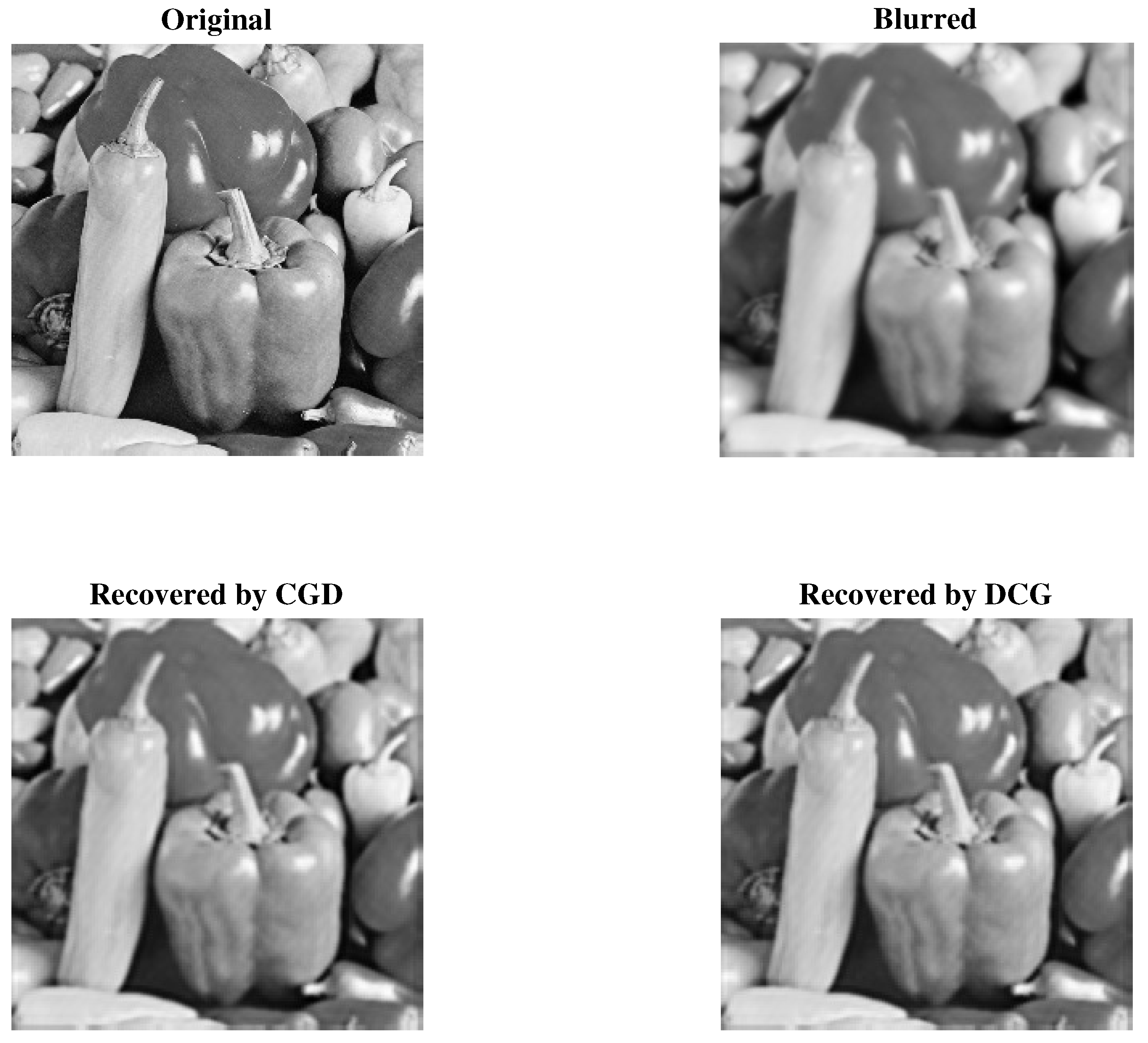
Applications in Compressive Sensing
4. Conclusions
Author Contributions
Funding
Acknowledgments
Conflicts of Interest
References
- Gu, B.; Sheng, V.S.; Tay, K.Y.; Romano, W.; Li, S. Incremental support vector learning for ordinal regression. IEEE Trans. Neural Netw. Learn. Syst. 2015, 26, 1403–1416. [Google Scholar] [CrossRef] [PubMed]
- Li, J.; Li, X.; Yang, B.; Sun, X. Segmentation-based image copy-move forgery detection scheme. IEEE Trans. Inf. Forensics Secur. 2015, 10, 507–518. [Google Scholar]
- Wen, X.; Shao, L.; Xue, Y.; Fang, W. A rapid learning algorithm for vehicle classification. Inf. Sci. 2015, 295, 395–406. [Google Scholar] [CrossRef]
- Michael, S.V.; Alfredo, I.N. Newton-type methods with generalized distances for constrained optimization. Optimization 1997, 41, 257–278. [Google Scholar]
- Figueiredo, M.A.T.; Nowak, R.D.; Wright, S.J. Gradient projection for sparse reconstruction: Application to compressed sensing and other inverse problems. IEEE J. Sel. Top. Signal Process. 2007, 1, 586–597. [Google Scholar] [CrossRef]
- Magnanti, T.L.; Perakis, G. Solving variational inequality and fixed point problems by line searches and potential optimization. Math. Program. 2004, 101, 435–461. [Google Scholar] [CrossRef]
- Pan, Z.; Zhang, Y.; Kwong, S. Efficient motion and disparity estimation optimization for low complexity multiview video coding. IEEE Trans. Broadcast. 2015, 61, 166–176. [Google Scholar]
- Xia, Z.; Wang, X.; Sun, X.; Wang, Q. A secure and dynamic multi-keyword ranked search scheme over encrypted cloud data. IEEE Trans. Parallel Distrib. Syst. 2016, 27, 340–352. [Google Scholar] [CrossRef]
- Zheng, Y.; Jeon, B.; Xu, D.; Wu, Q.M.; Zhang, H. Image segmentation by generalized hierarchical fuzzy c-means algorithm. J. Intell. Fuzzy Syst. 2015, 28, 961–973. [Google Scholar]
- Solodov, M.V.; Svaiter, B.F. A globally convergent inexact newton method for systems of monotone equations. In Reformulation: Nonsmooth, Piecewise Smooth, Semismooth and Smoothing Methods; Springer: Dordrecht, The Netherlands, 1998; pp. 355–369. [Google Scholar]
- Mohammad, H.; Abubakar, A.B. A positive spectral gradient-like method for nonlinear monotone equations. Bull. Comput. Appl. Math. 2017, 5, 99–115. [Google Scholar]
- Zhang, L.; Zhou, W. Spectral gradient projection method for solving nonlinear monotone equations. J. Comput. Appl. Math. 2006, 196, 478–484. [Google Scholar] [CrossRef]
- Zhou, W.J.; Li, D.H. A globally convergent BFGS method for nonlinear monotone equations without any merit functions. Math. Comput. 2008, 77, 2231–2240. [Google Scholar] [CrossRef]
- Zhou, W.; Li, D. Limited memory BFGS method for nonlinear monotone equations. J. Comput. Math. 2007, 25, 89–96. [Google Scholar]
- Abubakar, A.B.; Waziria, M.Y. A matrix-free approach for solving systems of nonlinear equations. J. Mod. Methods Numer. Math. 2016, 7, 1–9. [Google Scholar] [CrossRef]
- Abubakar, A.B.; Kumam, P. An improved three-term derivative-free method for solving nonlinear equations. Comput. Appl. Math. 2018, 37, 6760–6773. [Google Scholar] [CrossRef]
- Abubakar, A.B.; Kumam, P.; Awwal, A.M. A descent dai-liao projection method for convex constrained nonlinear monotone equations with applications. Thai J. Math. 2018, 17, 128–152. [Google Scholar]
- Wang, C.; Wang, Y.; Xu, C. A projection method for a system of nonlinear monotone equations with convex constraints. Math. Methods Oper. Res. 2007, 66, 33–46. [Google Scholar] [CrossRef]
- Xiao, Y.; Zhu, H. A conjugate gradient method to solve convex constrained monotone equations with applications in compressive sensing. J. Math. Anal. Appl. 2013, 405, 310–319. [Google Scholar] [CrossRef]
- Hager, W.; Zhang, H. A new conjugate gradient method with guaranteed descent and an efficient line search. SIAM J. Optim. 2005, 16, 170–192. [Google Scholar] [CrossRef]
- Liu, S.-Y.; Huang, Y.-Y.; Jiao, H.-W. Sufficient descent conjugate gradient methods for solving convex constrained nonlinear monotone equations. Abstr. Appl. Anal. 2014, 2014, 305643. [Google Scholar] [CrossRef]
- Liu, J.K.; Li, S.J. A projection method for convex constrained monotone nonlinear equations with applications. Comput. Math. Appl. 2015, 70, 2442–2453. [Google Scholar] [CrossRef]
- Ding, Y.; Xiao, Y.; Li, J. A class of conjugate gradient methods for convex constrained monotone equations. Optimization 2017, 66, 2309–2328. [Google Scholar] [CrossRef]
- Liu, J.; Feng, Y. A derivative-free iterative method for nonlinear monotone equations with convex constraints. Numer. Algorithms 2018, 1–18. [Google Scholar] [CrossRef]
- Muhammed, A.A.; Kumam, P.; Abubakar, A.B.; Wakili, A.; Pakkaranang, N. A new hybrid spectral gradient projection method for monotone system of nonlinear equations with convex constraints. Thai J. Math. 2018, 16, 125–147. [Google Scholar]
- La Cruz, W.; Martínez, J.; Raydan, M. Spectral residual method without gradient information for solving large-scale nonlinear systems of equations. Math. Comput. 2006, 75, 1429–1448. [Google Scholar] [CrossRef]
- Bing, Y.; Lin, G. An efficient implementation of Merrill’s method for sparse or partially separable systems of nonlinear equations. SIAM J. Optim. 1991, 1, 206–221. [Google Scholar] [CrossRef]
- Yu, Z.; Lin, J.; Sun, J.; Xiao, Y.H.; Liu, L.Y.; Li, Z.H. Spectral gradient projection method for monotone nonlinear equations with convex constraints. Appl. Numer. Math. 2009, 59, 2416–2423. [Google Scholar] [CrossRef]
- Yamashita, N.; Fukushima, M. Modified Newton methods for solving a semismooth reformulation of monotone complementarity problems. Math. Program. 1997, 76, 469–491. [Google Scholar] [CrossRef]
- Dolan, E.D.; Moré, J.J. Benchmarking optimization software with performance profiles. Math. Program. 2002, 91, 201–213. [Google Scholar] [CrossRef]
- Figueiredo, M.A.T.; Nowak, R.D. An EM algorithm for wavelet-based image restoration. IEEE Trans. Image Process. 2003, 12, 906–916. [Google Scholar] [CrossRef]
- Hale, E.T.; Yin, W.; Zhang, Y. A Fixed-Point Continuation Method for ℓ1-Regularized Minimization with Applications to Compressed Sensing; CAAM TR07-07; Rice University: Houston, TX, USA, 2007; pp. 43–44. [Google Scholar]
- Beck, A.; Teboulle, M. A fast iterative shrinkage-thresholding algorithm for linear inverse problems. SIAM J. Imaging Sci. 2009, 2, 183–202. [Google Scholar] [CrossRef]
- Van Den Berg, E.; Friedlander, M.P. Probing the pareto frontier for basis pursuit solutions. SIAM J. Sci. Comput. 2008, 31, 890–912. [Google Scholar] [CrossRef]
- Birgin, E.G.; Martínez, J.M.; Raydan, M. Nonmonotone spectral projected gradient methods on convex sets. SIAM J. Optim. 2000, 10, 1196–1211. [Google Scholar] [CrossRef]
- Xiao, Y.; Wang, Q.; Hu, Q. Non-smooth equations based method for ℓ1-norm problems with applications to compressed sensing. Nonlinear Anal. Theory Methods Appl. 2011, 74, 3570–3577. [Google Scholar] [CrossRef]
- Pang, J.-S. Inexact Newton methods for the nonlinear complementarity problem. Math. Program. 1986, 36, 54–71. [Google Scholar] [CrossRef]
- Wang, Z.; Bovik, A.C.; Sheikh, H.R.; Simoncelli, E.P. Image quality assessment: From error visibility to structural similarity. IEEE Trans. Image Process. 2004, 13, 600–612. [Google Scholar] [CrossRef]


| Algorithm 1 | PCG | PDY | |||||||||||
|---|---|---|---|---|---|---|---|---|---|---|---|---|---|
| DIMENSION | INITIAL POINT | ITER | FVAL | TIME | NORM | ITER | FVAL | TIME | NORM | ITER | FVAL | TIME | NORM |
| 1000 | 11 | 49 | 0.025557 | 8.88 | 18 | 73 | 0.019295 | 5.72 | 12 | 49 | 0.16248 | 9.18 | |
| 12 | 53 | 0.014164 | 4.78 | 18 | 73 | 0.011648 | 9.82 | 13 | 53 | 0.03780 | 6.35 | ||
| 12 | 53 | 0.008524 | 8.75 | 19 | 77 | 0.011197 | 7.1 | 14 | 57 | 0.01550 | 5.59 | ||
| 13 | 57 | 0.011333 | 6.68 | 18 | 73 | 0.022197 | 8.27 | 15 | 61 | 0.01746 | 4.07 | ||
| 13 | 57 | 0.014202 | 6.09 | 63 | 254 | 0.046072 | 9.58 | 14 | 57 | 0.02193 | 9.91 | ||
| 13 | 57 | 0.011045 | 8.14 | 61 | 246 | 0.031608 | 9.15 | 40 | 162 | 0.03472 | 9.70 | ||
| 5000 | 12 | 53 | 0.024311 | 5.82 | 18 | 73 | 0.11431 | 7.42 | 13 | 53 | 0.03158 | 6.87 | |
| 13 | 57 | 0.027361 | 3.13 | 19 | 77 | 0.03997 | 6.53 | 14 | 57 | 0.04270 | 4.62 | ||
| 13 | 57 | 0.02541 | 5.73 | 20 | 81 | 0.056159 | 5.2 | 15 | 61 | 0.05433 | 4.18 | ||
| 14 | 61 | 0.032038 | 4.38 | 19 | 77 | 0.038381 | 8.1 | 15 | 61 | 0.04357 | 9.08 | ||
| 14 | 61 | 0.039044 | 3.98 | 62 | 250 | 0.15836 | 9.53 | 15 | 61 | 0.08960 | 7.30 | ||
| 14 | 61 | 0.027231 | 5.33 | 60 | 242 | 0.13276 | 9.1 | 39 | 158 | 0.11284 | 9.86 | ||
| 10,000 | 12 | 53 | 0.05434 | 8.23 | 18 | 73 | 0.073207 | 9.5 | 13 | 53 | 0.06371 | 9.70 | |
| 13 | 57 | 0.045664 | 4.43 | 19 | 77 | 0.090771 | 8.15 | 14 | 57 | 0.06336 | 6.53 | ||
| 13 | 57 | 0.041922 | 8.09 | 20 | 81 | 0.070859 | 6.74 | 15 | 61 | 0.06414 | 5.90 | ||
| 14 | 61 | 0.047641 | 6.2 | 20 | 81 | 0.087357 | 5.11 | 16 | 65 | 0.07920 | 4.28 | ||
| 14 | 61 | 0.045734 | 5.62 | 62 | 250 | 0.24646 | 8.87 | 39 | 158 | 0.22101 | 7.97 | ||
| 14 | 61 | 0.057104 | 7.54 | 59 | 238 | 0.19949 | 9.96 | 87 | 351 | 0.36237 | 9.93 | ||
| 50,000 | 13 | 57 | 0.16384 | 5.41 | 19 | 77 | 0.25487 | 8.8 | 14 | 57 | 0.27607 | 7.12 | |
| 13 | 57 | 0.18633 | 9.9 | 20 | 81 | 0.32689 | 7.39 | 15 | 61 | 0.26220 | 4.91 | ||
| 14 | 61 | 0.20801 | 5.32 | 21 | 85 | 0.33649 | 6.31 | 16 | 65 | 0.28260 | 4.37 | ||
| 15 | 65 | 0.1946 | 4.08 | 21 | 85 | 0.32779 | 5.1 | 38 | 154 | 0.60650 | 7.54 | ||
| 15 | 65 | 0.19799 | 3.69 | 61 | 246 | 0.82615 | 8.85 | 177 | 712 | 2.52330 | 9.44 | ||
| 15 | 65 | 0.22418 | 4.95 | 59 | 238 | 0.79992 | 8.5 | 361 | 1449 | 5.97950 | 9.74 | ||
| 100,000 | 13 | 57 | 0.32291 | 7.65 | 20 | 81 | 0.53846 | 5.52 | 15 | 61 | 0.39342 | 3.39 | |
| 14 | 61 | 0.33329 | 4.12 | 21 | 85 | 0.61533 | 4.62 | 15 | 61 | 0.42154 | 6.94 | ||
| 14 | 61 | 0.37048 | 7.52 | 21 | 85 | 0.53638 | 8.78 | 16 | 65 | 0.45851 | 6.18 | ||
| 15 | 65 | 0.36058 | 5.76 | 21 | 85 | 0.62002 | 7.21 | 175 | 704 | 4.36100 | 9.47 | ||
| 15 | 65 | 0.34975 | 5.22 | 60 | 242 | 1.4564 | 9.73 | 176 | 708 | 4.29180 | 9.91 | ||
| 15 | 65 | 0.3621 | 7.01 | 58 | 234 | 1.4155 | 9.42 | 360 | 1445 | 9.71190 | 9.99 | ||
| Algorithm 1 | PCG | PDY | |||||||||||
|---|---|---|---|---|---|---|---|---|---|---|---|---|---|
| DIMENSION | INITIAL POINT | ITER | FVAL | TIME | NORM | ITER | FVAL | TIME | NORM | ITER | FVAL | TIME | NORM |
| 1000 | 9 | 38 | 3.1744 | 5.84 | 15 | 59 | 0.049899 | 8.59 | 10 | 39 | 0.01053 | 6.96 | |
| 10 | 42 | 0.014633 | 6.25 | 11 | 42 | 0.015089 | 9.07 | 11 | 43 | 0.00937 | 9.23 | ||
| 9 | 38 | 0.017067 | 7.4 | 17 | 66 | 0.016935 | 6.44 | 13 | 51 | 0.01111 | 6.26 | ||
| 7 | 30 | 0.006392 | 6.53 | 18 | 69 | 0.01436 | 6 | 14 | 55 | 0.02154 | 9.46 | ||
| 11 | 46 | 0.011954 | 3.47 | 13 | 48 | 0.00907 | 7.58 | 15 | 59 | 0.01850 | 4.60 | ||
| 12 | 50 | 0.68666 | 6.74 | 18 | 68 | 0.01352 | 5.4 | 15 | 59 | 0.01938 | 7.71 | ||
| 5000 | 10 | 42 | 0.11241 | 3.53 | 16 | 63 | 0.041151 | 9.35 | 11 | 43 | 0.03528 | 4.86 | |
| 11 | 46 | 0.028723 | 3.81 | 12 | 46 | 0.028706 | 8.8 | 12 | 47 | 0.04032 | 6.89 | ||
| 10 | 42 | 0.029367 | 4.3 | 18 | 70 | 0.047532 | 6.98 | 14 | 55 | 0.04889 | 4.61 | ||
| 13 | 54 | 0.036231 | 3.67 | 19 | 73 | 0.052164 | 6.45 | 15 | 59 | 0.04826 | 6.96 | ||
| 11 | 46 | 0.04963 | 7.21 | 14 | 52 | 0.040529 | 6.71 | 16 | 63 | 0.05969 | 3.37 | ||
| 13 | 54 | 0.054971 | 4.05 | 19 | 72 | 0.12303 | 5.71 | 16 | 63 | 0.06253 | 5.64 | ||
| 10,000 | 10 | 42 | 0.049614 | 4.98 | 17 | 67 | 0.074779 | 6.6 | 11 | 43 | 0.06732 | 6.85 | |
| 11 | 46 | 0.061595 | 5.36 | 13 | 50 | 0.08308 | 6.11 | 12 | 47 | 0.12232 | 9.72 | ||
| 10 | 42 | 0.054587 | 6.02 | 18 | 70 | 0.085554 | 9.83 | 14 | 55 | 0.08288 | 6.51 | ||
| 13 | 54 | 0.073333 | 5.16 | 19 | 73 | 0.10579 | 9.07 | 15 | 59 | 0.08413 | 9.82 | ||
| 12 | 50 | 0.06306 | 2.83 | 14 | 52 | 0.074982 | 9.18 | 16 | 63 | 0.09589 | 4.75 | ||
| 13 | 54 | 0.062259 | 5.69 | 19 | 72 | 0.099167 | 8.02 | 16 | 64 | 0.11499 | 8.55 | ||
| 50,000 | 11 | 46 | 0.20703 | 3.1 | 18 | 71 | 0.39473 | 7.37 | 12 | 47 | 0.27826 | 5.23 | |
| 12 | 50 | 0.23251 | 3.35 | 14 | 54 | 0.27346 | 6.74 | 13 | 51 | 0.29642 | 7.11 | ||
| 11 | 46 | 0.21338 | 3.73 | 20 | 78 | 0.37249 | 5.5 | 15 | 59 | 0.35602 | 4.82 | ||
| 14 | 58 | 0.3232 | 3.22 | 21 | 81 | 0.37591 | 5.07 | 35 | 141 | 0.69470 | 6.69 | ||
| 12 | 50 | 0.22703 | 6.27 | 16 | 60 | 0.26339 | 5.02 | 35 | 141 | 0.68488 | 9.12 | ||
| 14 | 58 | 0.25979 | 3.54 | 20 | 76 | 0.33814 | 8.93 | 35 | 141 | 0.70973 | 9.91 | ||
| 100,000 | 11 | 46 | 0.55511 | 4.38 | 19 | 75 | 0.65494 | 5.22 | 12 | 47 | 0.44541 | 7.39 | |
| 12 | 50 | 0.54694 | 4.73 | 14 | 54 | 0.4944 | 9.52 | 14 | 55 | 0.53299 | 3.39 | ||
| 11 | 46 | 0.40922 | 5.27 | 20 | 78 | 0.78319 | 7.78 | 15 | 60 | 0.58603 | 8.71 | ||
| 14 | 58 | 0.62049 | 4.55 | 21 | 81 | 0.76051 | 7.17 | 72 | 290 | 2.70630 | 8.31 | ||
| 12 | 50 | 0.47039 | 8.86 | 16 | 60 | 0.58545 | 7.07 | 72 | 290 | 2.72220 | 8.68 | ||
| 14 | 58 | 0.71174 | 5.01 | 21 | 80 | 0.77051 | 6.32 | 72 | 290 | 2.75850 | 8.96 | ||
| Algorithm 1 (DCG) | PCG | PDY | |||||||||||
|---|---|---|---|---|---|---|---|---|---|---|---|---|---|
| DIMENSION | INITIAL POINT | ITER | FVAL | TIME | NORM | ITER | FVAL | TIME | NORM | ITER | FVAL | TIME | NORM |
| 1000 | 10 | 43 | 0.75322 | 9.9 | 19 | 76 | 0.55752 | 5.62 | 12 | 48 | 0.01255 | 4.45 | |
| 11 | 47 | 0.006933 | 5.46 | 20 | 80 | 0.010936 | 5.58 | 12 | 48 | 0.01311 | 9.02 | ||
| 12 | 51 | 0.00676 | 3.48 | 21 | 84 | 0.011048 | 6.58 | 13 | 52 | 0.01486 | 8.34 | ||
| 12 | 51 | 0.009664 | 4.41 | 22 | 88 | 0.011058 | 5.67 | 14 | 56 | 0.01698 | 8.04 | ||
| 11 | 47 | 0.010487 | 9.06 | 22 | 88 | 0.012198 | 5.64 | 14 | 56 | 0.01551 | 9.72 | ||
| 13 | 55 | 0.012702 | 3.15 | 21 | 84 | 0.018231 | 8.36 | 14 | 56 | 0.01534 | 9.42 | ||
| 5000 | 11 | 47 | 0.019458 | 6.19 | 20 | 80 | 0.040808 | 6.29 | 12 | 48 | 0.03660 | 9.94 | |
| 12 | 51 | 0.021562 | 3.42 | 21 | 84 | 0.06688 | 6.25 | 13 | 52 | 0.03616 | 6.85 | ||
| 12 | 51 | 0.024274 | 7.79 | 22 | 88 | 0.04144 | 7.37 | 14 | 56 | 0.04594 | 6.14 | ||
| 12 | 51 | 0.026771 | 9.86 | 23 | 92 | 0.052214 | 6.35 | 15 | 60 | 0.04342 | 6.01 | ||
| 12 | 51 | 0.026814 | 5.67 | 23 | 92 | 0.041444 | 6.31 | 15 | 60 | 0.04296 | 7.25 | ||
| 13 | 55 | 0.023903 | 7.03 | 22 | 88 | 0.040135 | 9.37 | 32 | 129 | 0.10081 | 8.85 | ||
| 10,000 | 11 | 47 | 0.044134 | 8.75 | 20 | 80 | 0.064312 | 8.9 | 13 | 52 | 0.06192 | 4.77 | |
| 12 | 51 | 0.051947 | 4.83 | 21 | 84 | 0.088102 | 8.84 | 13 | 52 | 0.06442 | 9.68 | ||
| 13 | 55 | 0.057291 | 3.08 | 23 | 92 | 0.07296 | 5.22 | 14 | 56 | 0.09499 | 8.69 | ||
| 13 | 55 | 0.055134 | 3.9 | 23 | 92 | 0.075265 | 8.99 | 15 | 60 | 0.07696 | 8.5 | ||
| 12 | 51 | 0.047551 | 8.02 | 23 | 92 | 0.073937 | 8.93 | 33 | 133 | 0.18625 | 6.45 | ||
| 13 | 55 | 0.055069 | 9.95 | 23 | 92 | 0.099888 | 6.64 | 33 | 133 | 0.15548 | 7.51 | ||
| 50,000 | 12 | 51 | 0.19938 | 5.47 | 21 | 84 | 0.27031 | 9.97 | 14 | 56 | 0.23642 | 3.51 | |
| 13 | 55 | 0.22499 | 3.02 | 22 | 88 | 0.2657 | 9.9 | 14 | 56 | 0.24813 | 7.12 | ||
| 13 | 55 | 0.19396 | 6.89 | 24 | 96 | 0.3246 | 5.85 | 15 | 60 | 0.27049 | 6.53 | ||
| 13 | 55 | 0.20259 | 8.72 | 25 | 100 | 0.32373 | 5.04 | 34 | 137 | 0.54545 | 7.13 | ||
| 13 | 55 | 0.19452 | 5.01 | 25 | 100 | 0.33764 | 5.01 | 68 | 274 | 1.02330 | 9.99 | ||
| 14 | 59 | 0.22015 | 6.22 | 24 | 96 | 0.33687 | 7.44 | 69 | 278 | 1.03810 | 8.05 | ||
| 100,000 | 12 | 51 | 0.39983 | 7.74 | 22 | 88 | 0.63809 | 7.06 | 14 | 56 | 0.45475 | 4.96 | |
| 13 | 55 | 0.32765 | 4.28 | 23 | 92 | 0.63458 | 7.02 | 15 | 60 | 0.49018 | 3.39 | ||
| 13 | 55 | 0.30133 | 9.75 | 24 | 96 | 0.71422 | 8.27 | 15 | 60 | 0.49016 | 9.24 | ||
| 14 | 59 | 0.42865 | 3.45 | 25 | 100 | 0.73524 | 7.13 | 139 | 559 | 4.03110 | 9.01 | ||
| 13 | 55 | 0.34512 | 7.09 | 25 | 100 | 0.70625 | 7.09 | 70 | 282 | 2.07100 | 8.54 | ||
| 14 | 59 | 0.40387 | 8.8 | 25 | 100 | 0.76777 | 5.27 | 139 | 559 | 4.02440 | 9.38 | ||
| Algorithm 1 | PCG | PDY | |||||||||||
|---|---|---|---|---|---|---|---|---|---|---|---|---|---|
| DIMENSION | INITIAL POINT | ITER | FVAL | TIME | NORM | ITER | FVAL | TIME | NORM | ITER | FVAL | TIME | NORM |
| 1000 | 10 | 43 | 0.15461 | 8.33 | 18 | 72 | 0.11853 | 9.93 | 12 | 48 | 0.00989 | 4.60 | |
| 11 | 47 | 0.006276 | 3.84 | 19 | 76 | 0.014318 | 8.75 | 12 | 48 | 0.00966 | 9.57 | ||
| 11 | 47 | 0.009859 | 3.91 | 20 | 80 | 0.0093776 | 7.15 | 13 | 52 | 0.00887 | 8.49 | ||
| 11 | 47 | 0.007976 | 5.21 | 47 | 189 | 0.023321 | 7.83 | 12 | 48 | 0.01207 | 5.83 | ||
| 12 | 51 | 0.008382 | 4.09 | 46 | 185 | 0.047105 | 9.76 | 29 | 117 | 0.05371 | 9.43 | ||
| 12 | 51 | 0.008645 | 3.32 | 41 | 165 | 0.027719 | 8.77 | 29 | 117 | 0.02396 | 6.65 | ||
| 5000 | 11 | 47 | 0.022024 | 5.21 | 20 | 80 | 0.029445 | 5.57 | 13 | 52 | 0.02503 | 3.49 | |
| 11 | 47 | 0.020587 | 8.59 | 20 | 80 | 0.033115 | 9.8 | 13 | 52 | 0.02626 | 7.24 | ||
| 11 | 47 | 0.023714 | 8.75 | 21 | 84 | 0.033318 | 8.01 | 14 | 56 | 0.03349 | 6.29 | ||
| 12 | 51 | 0.024728 | 3.26 | 49 | 197 | 0.071715 | 9.46 | 13 | 52 | 0.02258 | 4.25 | ||
| 12 | 51 | 0.031015 | 9.14 | 49 | 197 | 0.068565 | 8.68 | 31 | 125 | 0.05471 | 7.59 | ||
| 12 | 51 | 0.030012 | 7.43 | 44 | 177 | 0.070862 | 7.79 | 63 | 254 | 0.10064 | 8.54 | ||
| 10,000 | 11 | 47 | 0.041476 | 7.37 | 20 | 80 | 0.043013 | 7.88 | 13 | 52 | 0.03761 | 4.93 | |
| 12 | 51 | 0.047866 | 3.4 | 21 | 84 | 0.051685 | 6.94 | 14 | 56 | 0.04100 | 3.37 | ||
| 12 | 51 | 0.042607 | 3.46 | 22 | 88 | 0.050422 | 5.67 | 14 | 56 | 0.03919 | 8.90 | ||
| 12 | 51 | 0.036406 | 4.61 | 50 | 201 | 0.17563 | 9.84 | 32 | 129 | 0.09613 | 6.02 | ||
| 13 | 55 | 0.041374 | 3.61 | 50 | 201 | 0.20035 | 9.03 | 32 | 129 | 0.09177 | 6.44 | ||
| 13 | 55 | 0.039847 | 2.94 | 45 | 181 | 0.12214 | 8.11 | 64 | 258 | 0.20791 | 9.39 | ||
| 50,000 | 12 | 51 | 0.13928 | 4.61 | 21 | 84 | 0.27145 | 8.83 | 14 | 56 | 0.17193 | 3.63 | |
| 12 | 51 | 0.18031 | 7.6 | 22 | 88 | 0.23149 | 7.78 | 14 | 56 | 0.15237 | 7.54 | ||
| 12 | 51 | 0.12526 | 7.74 | 23 | 92 | 0.28789 | 6.36 | 15 | 60 | 0.16549 | 6.66 | ||
| 13 | 55 | 0.14322 | 2.88 | 53 | 213 | 0.61624 | 8.75 | 67 | 270 | 0.76283 | 7.81 | ||
| 13 | 55 | 0.17904 | 8.08 | 53 | 213 | 0.7119 | 8.02 | 67 | 270 | 0.76157 | 8.80 | ||
| 13 | 55 | 0.13635 | 6.57 | 47 | 189 | 0.48192 | 9.8 | 269 | 1080 | 2.92510 | 9.41 | ||
| 100,000 | 12 | 51 | 0.24293 | 6.52 | 22 | 88 | 0.60822 | 6.25 | 14 | 56 | 0.30229 | 5.13 | |
| 13 | 55 | 0.27433 | 3.01 | 23 | 92 | 0.52965 | 5.51 | 15 | 60 | 0.31648 | 3.59 | ||
| 13 | 55 | 0.2714 | 3.06 | 23 | 92 | 0.57064 | 8.99 | 32 | 129 | 0.72838 | 9.99 | ||
| 13 | 55 | 0.26819 | 4.08 | 54 | 217 | 1.1805 | 9.1 | 135 | 543 | 2.86780 | 9.73 | ||
| 14 | 59 | 0.31696 | 3.2 | 54 | 217 | 1.107 | 8.34 | 272 | 1092 | 5.74140 | 9.91 | ||
| 13 | 55 | 0.2698 | 9.29 | 49 | 197 | 1.0617 | 7.49 | 548 | 2197 | 11.44130 | 9.87 | ||
| Algorithm 1 | PCG | PDY | |||||||||||
|---|---|---|---|---|---|---|---|---|---|---|---|---|---|
| DIMENSION | INITIAL POINT | ITER | FVAL | TIME | NORM | ITER | FVAL | TIME | NORM | ITER | FVAL | TIME | NORM |
| 1000 | 19 | 78 | 0.71709 | 8.63 | 22 | 83 | 0.099338 | 7.48 | 16 | 63 | 0.07575 | 6.03 | |
| 21 | 86 | 0.017127 | 7.65 | 23 | 88 | 0.016014 | 7.31 | 16 | 63 | 0.01470 | 5.42 | ||
| 23 | 95 | 0.013909 | 7.23 | 23 | 90 | 0.016328 | 9.31 | 33 | 132 | 0.02208 | 6.75 | ||
| 22 | 92 | 0.0165 | 8.64 | 49 | 197 | 0.030124 | 8.45 | 30 | 121 | 0.01835 | 8.39 | ||
| 35 | 145 | 0.024702 | 8.26 | 53 | 213 | 0.039321 | 8.38 | 32 | 129 | 0.02700 | 8.47 | ||
| 43 | 182 | 0.027471 | 8.7 | 46 | 185 | 0.033627 | 8.8 | 30 | 121 | 0.01712 | 6.95 | ||
| 5000 | 146 | 592 | 0.23803 | 9.45 | 24 | 91 | 0.060158 | 6.36 | 17 | 67 | 0.04394 | 5.64 | |
| 21 | 86 | 0.04337 | 9.46 | 25 | 95 | 0.060385 | 6.24 | 17 | 67 | 0.04635 | 5.07 | ||
| 24 | 99 | 0.054619 | 8.27 | 25 | 98 | 0.040015 | 5.86 | 35 | 140 | 0.08311 | 9.74 | ||
| 24 | 100 | 0.066424 | 6.66 | 53 | 213 | 0.098097 | 9.11 | 33 | 133 | 0.08075 | 6.02 | ||
| 38 | 157 | 0.071222 | 9.28 | 58 | 233 | 0.10958 | 8.56 | 35 | 141 | 0.10091 | 7.51 | ||
| 45 | 190 | 0.090276 | 7.14 | 50 | 201 | 0.21521 | 7.65 | 32 | 129 | 0.08054 | 8.55 | ||
| 10,000 | 211 | 853 | 0.60357 | 9.65 | 25 | 95 | 0.076427 | 5.4 | 17 | 67 | 0.06816 | 8.81 | |
| 22 | 90 | 0.08012 | 4.98 | 25 | 95 | 0.098461 | 8.9 | 17 | 67 | 0.08833 | 7.80 | ||
| 25 | 103 | 0.089269 | 5.89 | 25 | 98 | 0.07495 | 8.64 | 37 | 148 | 0.14732 | 6.36 | ||
| 25 | 104 | 0.11781 | 5.54 | 55 | 221 | 0.19048 | 9.11 | 37 | 149 | 0.14293 | 8.25 | ||
| 40 | 165 | 0.15859 | 7.43 | 60 | 241 | 0.19751 | 9.01 | 36 | 145 | 0.14719 | 8.23 | ||
| 46 | 194 | 0.1728 | 8.62 | 51 | 205 | 0.28882 | 9.62 | 74 | 298 | 0.26456 | 7.79 | ||
| 50,000 | 225 | 909 | 2.1373 | 9.93 | 26 | 99 | 0.34575 | 6.75 | 42 | 169 | 0.58113 | 7.78 | |
| 23 | 94 | 0.31098 | 4.48 | 27 | 103 | 0.43806 | 5.16 | 42 | 169 | 0.58456 | 7.13 | ||
| 26 | 107 | 0.36293 | 6.83 | 27 | 106 | 0.4815 | 5.28 | 41 | 165 | 0.58717 | 8.87 | ||
| 26 | 108 | 0.32427 | 9.72 | 60 | 241 | 0.90868 | 8.66 | 40 | 161 | 0.56431 | 7.17 | ||
| 43 | 177 | 0.48938 | 9.47 | 65 | 261 | 0.7924 | 9.05 | 82 | 330 | 1.08920 | 8.44 | ||
| 50 | 210 | 0.69117 | 8.12 | 56 | 225 | 0.72334 | 8.19 | 80 | 322 | 1.06670 | 7.82 | ||
| 100,000 | 231 | 933 | 4.2588 | 9.85 | 26 | 99 | 0.71242 | 9.73 | 43 | 173 | 1.09620 | 8.47 | |
| 139 | 564 | 2.7266 | 9.96 | 27 | 103 | 0.62746 | 7.39 | 43 | 173 | 1.10040 | 7.77 | ||
| 26 | 107 | 0.57505 | 9.92 | 27 | 106 | 0.82989 | 7.77 | 42 | 169 | 1.08330 | 9.66 | ||
| 27 | 112 | 0.62227 | 8.52 | 62 | 249 | 1.5474 | 9 | 85 | 342 | 2.11880 | 9.22 | ||
| 45 | 185 | 0.8992 | 7.79 | 67 | 269 | 1.6692 | 9.5 | 84 | 338 | 2.10640 | 9.78 | ||
| 52 | 218 | 1.4318 | 7.37 | 58 | 233 | 1.4333 | 8.32 | 167 | 671 | 4.06200 | 9.90 | ||
| Algorithm 1 | PCG | PDY | |||||||||||
|---|---|---|---|---|---|---|---|---|---|---|---|---|---|
| DIMENSION | INITIAL POINT | ITER | FVAL | TIME | NORM | ITER | FVAL | TIME | NORM | ITER | FVAL | TIME | NORM |
| 1000 | 13 | 55 | 1.38 | 5.68 | 23 | 92 | 0.4038 | 9.28 | 15 | 60 | 0.01671 | 4.35 | |
| 13 | 55 | 0.013339 | 5.47 | 23 | 92 | 0.016325 | 8.92 | 15 | 60 | 0.01346 | 4.18 | ||
| 13 | 55 | 0.066142 | 4.81 | 23 | 92 | 0.023045 | 7.86 | 15 | 60 | 0.01630 | 3.68 | ||
| 13 | 55 | 0.026838 | 3.3 | 23 | 92 | 0.016172 | 5.38 | 14 | 56 | 0.01339 | 7.48 | ||
| 12 | 51 | 0.009864 | 9.45 | 22 | 88 | 0.03785 | 8.62 | 14 | 56 | 0.01267 | 6.01 | ||
| 12 | 51 | 0.009881 | 5.57 | 22 | 88 | 0.015013 | 5.08 | 14 | 56 | 0.01685 | 3.54 | ||
| 5000 | 14 | 59 | 0.042533 | 3.56 | 25 | 100 | 0.061642 | 5.22 | 15 | 60 | 0.05038 | 9.73 | |
| 14 | 59 | 0.036648 | 3.43 | 25 | 100 | 0.092952 | 5.02 | 15 | 60 | 0.04775 | 9.36 | ||
| 14 | 59 | 0.043452 | 3.02 | 24 | 96 | 0.068141 | 8.82 | 15 | 60 | 0.04923 | 8.25 | ||
| 13 | 55 | 0.032579 | 7.38 | 24 | 96 | 0.084625 | 6.04 | 15 | 60 | 0.05793 | 5.64 | ||
| 13 | 55 | 0.03295 | 5.92 | 23 | 92 | 0.086122 | 9.67 | 15 | 60 | 0.04597 | 4.53 | ||
| 13 | 55 | 0.033062 | 3.49 | 23 | 92 | 0.093318 | 5.7 | 14 | 56 | 0.05070 | 7.93 | ||
| 10,000 | 14 | 59 | 0.064917 | 5.04 | 25 | 100 | 0.21424 | 7.38 | 68 | 274 | 0.40724 | 9.06 | |
| 14 | 59 | 0.069913 | 4.84 | 25 | 100 | 0.13978 | 7.09 | 68 | 274 | 0.41818 | 8.72 | ||
| 14 | 59 | 0.08473 | 4.27 | 25 | 100 | 0.1731 | 6.25 | 34 | 137 | 0.21905 | 6.22 | ||
| 14 | 59 | 0.075847 | 2.92 | 24 | 96 | 0.14744 | 8.54 | 15 | 60 | 0.10076 | 7.98 | ||
| 13 | 55 | 0.07974 | 8.38 | 24 | 96 | 0.14169 | 6.85 | 15 | 60 | 0.12680 | 6.40 | ||
| 13 | 55 | 0.063129 | 4.94 | 23 | 92 | 0.15294 | 8.06 | 15 | 60 | 0.11984 | 3.78 | ||
| 50,000 | 15 | 63 | 0.25329 | 3.15 | 26 | 104 | 0.64669 | 8.26 | 143 | 575 | 3.09120 | 9.42 | |
| 15 | 63 | 0.36394 | 3.03 | 26 | 104 | 0.67717 | 7.95 | 143 | 575 | 3.06200 | 9.06 | ||
| 14 | 59 | 0.2413 | 9.54 | 26 | 104 | 0.5562 | 7 | 142 | 571 | 3.04950 | 9.04 | ||
| 14 | 59 | 0.27502 | 6.53 | 25 | 100 | 0.56171 | 9.56 | 69 | 278 | 1.53920 | 9.14 | ||
| 14 | 59 | 0.36404 | 5.24 | 25 | 100 | 0.57982 | 7.67 | 68 | 274 | 1.49490 | 9.43 | ||
| 14 | 59 | 0.2506 | 3.09 | 24 | 96 | 0.58645 | 9.03 | 15 | 60 | 0.38177 | 8.44 | ||
| 100,000 | 15 | 63 | 0.84781 | 4.45 | 27 | 108 | 1.3215 | 5.86 | 292 | 1172 | 13.59530 | 9.53 | |
| 15 | 63 | 0.66663 | 4.28 | 27 | 108 | 1.5062 | 5.63 | 290 | 1164 | 13.30930 | 9.75 | ||
| 15 | 63 | 0.66683 | 3.77 | 26 | 104 | 1.166 | 9.9 | 144 | 579 | 6.68150 | 9.96 | ||
| 14 | 59 | 0.62697 | 9.24 | 26 | 104 | 1.3961 | 6.78 | 141 | 567 | 6.50800 | 9.92 | ||
| 14 | 59 | 0.62891 | 7.41 | 26 | 104 | 1.2711 | 5.44 | 70 | 282 | 3.30510 | 8.07 | ||
| 14 | 59 | 0.62422 | 4.37 | 25 | 100 | 1.1685 | 6.4 | 34 | 137 | 1.64510 | 6.37 | ||
| Algorithm 1 | PCG | PDY | |||||||||||
|---|---|---|---|---|---|---|---|---|---|---|---|---|---|
| DIMENSION | INITIAL POINT | ITER | FVAL | TIME | NORM | ITER | FVAL | TIME | NORM | ITER | FVAL | TIME | NORM |
| 1000 | 6 | 28 | 0.25689 | 2 | 17 | 69 | 1.2275 | 6.98 | 14 | 57 | 0.00953 | 5.28 | |
| 6 | 28 | 0.008469 | 1.26 | 15 | 61 | 0.23396 | 9.89 | 13 | 53 | 0.00896 | 9.05 | ||
| 4 | 20 | 0.003619 | 9.25 | 16 | 65 | 0.008095 | 5.79 | 3 | 12 | 0.00426 | 8.47 | ||
| 5 | 24 | 0.004345 | 5.7 | 16 | 65 | 0.010077 | 5.21 | 15 | 61 | 0.01169 | 6.73 | ||
| 6 | 28 | 0.007146 | 4.42 | 19 | 77 | 0.05354 | 4.95 | 31 | 126 | 0.03646 | 9.03 | ||
| 6 | 27 | 0.004299 | 4.43 | 18 | 72 | 0.025677 | 8.93 | 15 | 60 | 0.01082 | 3.99 | ||
| 5000 | 6 | 28 | 0.012915 | 4.47 | 18 | 73 | 0.17722 | 7.6 | 15 | 61 | 0.03215 | 4.25 | |
| 6 | 28 | 0.012272 | 2.81 | 17 | 69 | 0.027729 | 5.25 | 14 | 57 | 0.02942 | 7.40 | ||
| 5 | 24 | 0.014669 | 1.16 | 17 | 69 | 0.02985 | 6.31 | 4 | 16 | 0.01107 | 1.01 | ||
| 6 | 28 | 0.012765 | 7.14 | 17 | 69 | 0.028176 | 5.68 | 16 | 65 | 0.04331 | 5.43 | ||
| 6 | 28 | 0.01331 | 9.89 | 20 | 81 | 0.032213 | 5.39 | 33 | 134 | 0.09379 | 7.78 | ||
| 6 | 27 | 0.015828 | 9.91 | 19 | 76 | 0.044328 | 9.73 | 15 | 60 | 0.04077 | 8.92 | ||
| 10,000 | 6 | 28 | 0.022346 | 6.32 | 19 | 77 | 0.17863 | 5.23 | 15 | 61 | 0.06484 | 6.01 | |
| 6 | 28 | 0.022669 | 3.97 | 17 | 69 | 0.049242 | 7.42 | 15 | 61 | 0.07734 | 3.77 | ||
| 5 | 24 | 0.039342 | 1.64 | 17 | 69 | 0.048238 | 8.92 | 4 | 16 | 0.02707 | 1.42 | ||
| 6 | 28 | 0.021017 | 1.01 | 17 | 69 | 0.04807 | 8.03 | 16 | 65 | 0.07941 | 7.69 | ||
| 7 | 32 | 0.031654 | 7.83 | 20 | 81 | 0.063156 | 7.62 | 34 | 138 | 0.14942 | 6.83 | ||
| 7 | 31 | 0.023456 | 7.85 | 20 | 80 | 0.059438 | 6.7 | 34 | 138 | 0.15224 | 8.81 | ||
| 50,000 | 7 | 32 | 0.092452 | 7.91 | 20 | 81 | 1.0808 | 5.7 | 16 | 65 | 0.25995 | 4.89 | |
| 6 | 28 | 0.1068 | 8.88 | 18 | 73 | 0.32804 | 8.08 | 15 | 61 | 0.24674 | 8.42 | ||
| 5 | 24 | 0.065684 | 3.66 | 18 | 73 | 0.2189 | 9.71 | 4 | 16 | 0.09405 | 3.18 | ||
| 6 | 28 | 0.10193 | 2.26 | 18 | 73 | 0.3497 | 8.75 | 36 | 146 | 0.55207 | 6.39 | ||
| 7 | 32 | 0.095676 | 1.75 | 21 | 85 | 0.22595 | 8.3 | 35 | 142 | 0.54679 | 9.05 | ||
| 7 | 31 | 0.092855 | 1.76 | 21 | 84 | 0.22374 | 7.3 | 36 | 146 | 0.55764 | 7.59 | ||
| 100,000 | 7 | 32 | 0.17597 | 1.12 | 20 | 81 | 2.1675 | 8.06 | 17 | 69 | 0.52595 | 5.68 | |
| 7 | 32 | 0.1741 | 7.03 | 19 | 77 | 0.45553 | 5.57 | 16 | 65 | 0.52102 | 4.34 | ||
| 5 | 24 | 0.17522 | 5.18 | 19 | 77 | 0.43219 | 6.69 | 4 | 16 | 0.14864 | 4.50 | ||
| 6 | 28 | 0.20785 | 3.19 | 19 | 77 | 0.52259 | 6.03 | 36 | 146 | 1.05360 | 9.04 | ||
| 7 | 32 | 0.23979 | 2.48 | 22 | 89 | 0.6171 | 5.72 | 74 | 299 | 2.10730 | 8.55 | ||
| 7 | 31 | 0.23128 | 2.48 | 22 | 88 | 0.57384 | 5.03 | 37 | 150 | 1.08240 | 6.66 | ||
| Algorithm 1 | PCG | PDY | |||||||||||
|---|---|---|---|---|---|---|---|---|---|---|---|---|---|
| DIMENSION | INITIAL POINT | ITER | FVAL | TIME | NORM | ITER | FVAL | TIME | NORM | ITER | FVAL | TIME | NORM |
| 1000 | 7 | 28 | 0.11495 | 3.03 | 9 | 32 | 0.85797 | 7.6 | 69 | 279 | 0.05538 | 8.95 | |
| 7 | 28 | 0.005034 | 3.03 | 9 | 32 | 0.034675 | 7.6 | 270 | 1085 | 0.18798 | 9.72 | ||
| 7 | 28 | 0.006743 | 3.03 | 9 | 32 | 0.005985 | 7.6 | 24 | 52 | 0.02439 | 6.57 | ||
| 7 | 28 | 0.005856 | 3.03 | 9 | 32 | 0.004808 | 7.6 | 27 | 58 | 0.01520 | 7.59 | ||
| 7 | 28 | 0.004635 | 3.03 | 9 | 32 | 0.015026 | 7.6 | 28 | 61 | 0.04330 | 9.21 | ||
| 7 | 28 | 0.006487 | 3.03 | 9 | 32 | 0.15778 | 7.6 | 40 | 85 | 0.02116 | 8.45 | ||
| 5000 | 5 | 22 | 0.009068 | 4.52 | 7 | 26 | 0.67239 | 1.3 | 658 | 2639 | 1.13030 | 9.98 | |
| 5 | 22 | 0.009369 | 4.52 | 7 | 26 | 0.010651 | 1.3 | 27 | 58 | 0.05101 | 7.59 | ||
| 5 | 22 | 0.010895 | 4.52 | 7 | 26 | 0.015758 | 1.3 | 49 | 104 | 0.08035 | 8.11 | ||
| 5 | 22 | 0.014958 | 4.52 | 7 | 26 | 0.014935 | 1.3 | 40 | 85 | 0.07979 | 8.45 | ||
| 5 | 22 | 0.01507 | 4.52 | 7 | 26 | 0.01524 | 1.3 | 18 | 40 | 0.09128 | 9.14 | ||
| 5 | 22 | 0.008716 | 4.52 | 7 | 26 | 0.1999 | 1.3 | 17 | 38 | 0.18528 | 8.98 | ||
| 10,000 | 6 | 27 | 0.031198 | 3.81 | 5 | 19 | 0.044387 | 5.06 | 49 | 104 | 0.20443 | 7.62 | |
| 6 | 27 | 0.02098 | 3.81 | 5 | 19 | 0.0223 | 5.06 | 40 | 85 | 0.15801 | 8.45 | ||
| 6 | 27 | 0.01991 | 3.81 | 5 | 19 | 0.018209 | 5.06 | 19 | 42 | 0.37880 | 7.66 | ||
| 6 | 27 | 0.025402 | 3.81 | 5 | 19 | 0.021654 | 5.06 | 90 | 187 | 1.25802 | 9.7 | ||
| 6 | 27 | 0.025816 | 3.81 | 5 | 19 | 0.017353 | 5.06 | 988 | 1988 | 12.68259 | 9.93 | ||
| 6 | 27 | 0.025065 | 3.81 | 5 | 19 | 0.019763 | 5.06 | 27 | 58 | 0.32859 | 7.59 | ||
| 50,000 | 4 | 21 | 0.083641 | 2.34 | 8 | 33 | 0.42902 | 5.15 | 19 | 42 | 0.52291 | 6.42 | |
| 4 | 21 | 0.074156 | 2.34 | 8 | 33 | 0.11525 | 5.15 | 148 | 304 | 3.93063 | 9.92 | ||
| 4 | 21 | 0.078596 | 2.34 | 8 | 33 | 0.14432 | 5.15 | 937 | 1886 | 22.97097 | 9.87 | ||
| 4 | 21 | 0.078289 | 2.34 | 8 | 33 | 0.11562 | 5.15 | 27 | 58 | 0.68467 | 7.59 | ||
| 4 | 21 | 0.073535 | 2.34 | 8 | 33 | 0.11674 | 5.15 | 346 | 702 | 8.45043 | 9.79 | ||
| 4 | 21 | 0.081909 | 2.34 | 8 | 33 | 0.10486 | 5.15 | 40 | 85 | 0.99230 | 8.45 | ||
| 100,000 | 4 | 22 | 0.1663 | 6.25 | 6 | 25 | 1.2922 | 6.81 | - | - | - | - | |
| 4 | 22 | 0.15147 | 6.25 | 6 | 25 | 0.18839 | 6.81 | - | - | - | - | ||
| 4 | 22 | 0.15582 | 6.25 | 6 | 25 | 0.16153 | 6.81 | - | - | - | - | ||
| 4 | 22 | 0.15465 | 6.25 | 6 | 25 | 0.17397 | 6.81 | - | - | - | - | ||
| 4 | 22 | 0.16744 | 6.25 | 6 | 25 | 0.18586 | 6.81 | - | - | - | - | ||
| 4 | 22 | 0.1687 | 6.25 | 6 | 25 | 0.17938 | 6.81 | - | - | - | - | ||
| Algorithm 1 | PCG | PDY | |||||||||||
|---|---|---|---|---|---|---|---|---|---|---|---|---|---|
| DIMENSION | INITIAL POINT | ITER | FVAL | TIME | NORM | ITER | FVAL | TIME | NORM | ITER | FVAL | TIME | NORM |
| 4 | 51 | 215 | 0.23665 | 9.01 | 79 | 321 | 0.5978 | 9.76 | 59 | 241 | 0.71268 | 9.36 | |
| 51 | 215 | 0.04968 | 9.99 | 77 | 313 | 0.016326 | 9.85 | 58 | 237 | 0.045441 | 9.73 | ||
| 53 | 223 | 0.017211 | 9.46 | 80 | 325 | 0.16529 | 9.38 | 59 | 241 | 0.019552 | 9.9 | ||
| 53 | 223 | 0.019004 | 9.68 | 83 | 337 | 0.041713 | 9.57 | 62 | 253 | 0.022007 | 8.07 | ||
| 57 | 239 | 0.023447 | 8.87 | 81 | 329 | 0.11972 | 9.04 | 61 | 249 | 0.040117 | 8.36 | ||
| 54 | 227 | 0.020832 | 9.31 | 82 | 333 | 0.016127 | 9.3 | 61 | 249 | 0.017374 | 9.18 | ||
| Image | Iter | ObjFun | MSE | SNR | ||||
|---|---|---|---|---|---|---|---|---|
| DCG | CGD | DCG | CGD | DCG | CGD | DCG | CGD | |
| P1(1E-8) | 8 | 9 | 4.397 | 4.398 | 3.136 | 3.157 | 9.42 | 9.39 |
| P1(1E-1) | 8 | 9 | 4.399 | 4.401 | 3.147 | 3.163 | 9.40 | 9.38 |
| P1(0.11) | 11 | 8 | 4.428 | 4.432 | 3.229 | 3.232 | 9.29 | 9.29 |
| P1(0.25) | 12 | 8 | 4.468 | 4.473 | 3.365 | 3.289 | 9.11 | 9.21 |
| P1(1E-8) | 9 | 9 | 4.555 | 4.556 | 3.287 | 3.3412 | 9.14 | 9.07 |
| P1(1E-1) | 9 | 9 | 4.558 | 4.559 | 3.298 | 3.348 | 9.12 | 9.06 |
| P1(0.11) | 12 | 12 | 4.588 | 4.591 | 3.416 | 3.446 | 8.97 | 8.93 |
| P1(0.25) | 7 | 8 | 4.628 | 4.630 | 3.621 | 3.500 | 8.72 | 8.86 |
| P1(1E-8) | 9 | 9 | 5.179 | 5.179 | 3.209 | 3.3259 | 10.03 | 9.96 |
| P1(1E-1) | 9 | 9 | 5.182 | 5.182 | 3.231 | 3.267 | 10.00 | 9.95 |
| P1(0.11) | 7 | 9 | 5.209 | 5.209 | 3.436 | 3.344 | 9.73 | 9.85 |
| P1(0.25) | 10 | 8 | 5.250 | 5.254 | 3.557 | 3.438 | 9.58 | 9.73 |
| P1(1E-8) | 9 | 9 | 4.388 | 4.389 | 3.299 | 3.335 | 9.03 | 8.99 |
| P1(1E-1) | 9 | 9 | 4.391 | 4.393 | 3.308 | 3.340 | 9.02 | 8.98 |
| P1(0.11) | 12 | 8 | 4.421 | 4.424 | 3.425 | 3.411 | 8.87 | 8.89 |
| P1(0.25) | 7 | 8 | 4.461 | 4.463 | 3.621 | 3.483 | 8.63 | 8.80 |
© 2019 by the authors. Licensee MDPI, Basel, Switzerland. This article is an open access article distributed under the terms and conditions of the Creative Commons Attribution (CC BY) license (http://creativecommons.org/licenses/by/4.0/).
Share and Cite
Abubakar, A.B.; Kumam, P.; Mohammad, H.; Awwal, A.M. An Efficient Conjugate Gradient Method for Convex Constrained Monotone Nonlinear Equations with Applications. Mathematics 2019, 7, 767. https://doi.org/10.3390/math7090767
Abubakar AB, Kumam P, Mohammad H, Awwal AM. An Efficient Conjugate Gradient Method for Convex Constrained Monotone Nonlinear Equations with Applications. Mathematics. 2019; 7(9):767. https://doi.org/10.3390/math7090767
Chicago/Turabian StyleAbubakar, Auwal Bala, Poom Kumam, Hassan Mohammad, and Aliyu Muhammed Awwal. 2019. "An Efficient Conjugate Gradient Method for Convex Constrained Monotone Nonlinear Equations with Applications" Mathematics 7, no. 9: 767. https://doi.org/10.3390/math7090767
APA StyleAbubakar, A. B., Kumam, P., Mohammad, H., & Awwal, A. M. (2019). An Efficient Conjugate Gradient Method for Convex Constrained Monotone Nonlinear Equations with Applications. Mathematics, 7(9), 767. https://doi.org/10.3390/math7090767