Optimization of Queueing Model with Server Heating and Cooling

Abstract

The operation of many real-world systems, e.g., servers of data centers, is accompanied by the heating of a server. Correspondingly, certain cooling mechanisms are used. If the server becomes overheated, it interrupts processing of customers and needs to be cooled. A customer is lost when its service is interrupted. To prevent overheating and reduce the customer loss probability, we suggest temporal termination of service of new customers when the temperature of the server reaches the predefined threshold value. Service is resumed after the temperature drops below another threshold value. The problem of optimal choice of the thresholds (with respect to the chosen economical criterion) is numerically solved under quite general assumptions about the parameters of the system (Markovian arrival process, phase-type distribution of service time, and accounting for customers impatience). Numerical examples are presented.

1. Introduction

The goal of operation of many real-world systems is to obtain profit via providing service to some customers. For example, in data centers, the profit is obtained via storing and retrieving the information for users on demand. The operation of such systems is possible only under fulfillment of various limitations. An important problem in organization of the operation of data centers is the effective cooling of servers. High performance servers generate a lot of heat and it is necessary to effectively cool the central processing unit, memory modules, power supplies, graphics processing units and other devices to avoid system overheating and premature failures (see, e.g., [1]).

It is clear that, to maximize the profit, it is necessary to use the power of the available server to a maximum extent. However, this may cause overheating of the server, the loss of a customer who was using the service during the overheating moment and a temporal termination of the service for cooling the server. To prevent overheating of the server during service, it sounds reasonable to stop new services if the temperature of the server reaches some level (threshold). Definitely, this threshold should be less than the critical level but more or less close to this level. Otherwise, a certain part of the server capacity is not utilized and this may lead to the loss of some profit. If service can be postponed or interrupted, it is necessary to specify when service will be resumed. This can be done by means of introducing one more threshold. Service is resumed when the temperature of the server is dropped to this threshold. It is obvious that this threshold should be less than the first threshold. The difference between the thresholds should not be too large. Otherwise, again, the server capacity is under-utilized. However, if the difference is too small, the bans and permissions to start new services can occur too frequently and this can be charged by a decision-maker. Therefore, the problem of optimal choice of the two thresholds is not trivial and challenging.

In this paper, we numerically solve this problem in the following way. Under any fixed pair of thresholds, the behavior of the system is described by a Markov chain. This Markov chain is multi-dimensional because it has to include the components defining the number of customers in the system, the current state of the server (idle, operating, or cooling) and its temperature, underlying processes of customer arrival and service processes. Due to the existence of periods when service is not provided, in our model, we account for the possible impatience of the customers waiting in the queue. Due to considering impatience, this Markov chain does not belong to the class of level-independent quasi-birth-and-death processes and its analysis is non-trivial. We use results from [2,3] for computation of the stationary probabilities of the states of the chain. Having the stationary probabilities computed, we derive formulas for computation of the main performance indicators of the system and the cost criterion for any fixed pair of the thresholds defining behavior of the system. This allows us to numerically solve the problem of choosing the optimal values of the thresholds.

The considered model is very close to the models in which some additional resource is required to provide service to a customer. These models include, in particular, so-called queueing/inventory models (see, e.g., [4]), queueing systems with energy harvesting (see, e.g., [5]), queueing models with paired customers (see [6]), assembly-like queue (see [7]), passenger-taxi or double-ended queues (see [8]), coupled queues (see [9]), etc. In our model, the role of the additional resource is played by the lag between the critical and current value of the server’s temperature. The essential difference between our model and the above mentioned models consists of the following. Usually, the additional resource has the influence on the behavior of the queueing system only at the potential service beginning moments. If the resource is available, the known required for service amount of the resource is reserved. Service starts and, then, successfully finishes. Otherwise, if the resource is not available at the potential service beginning moment, service is cancelled or postponed until the required amount of the additional resource becomes available. In our model, we have a more complicated situation: the “additional resource” has a permanent influence on the behavior of the queueing system. Required for a customer service amount of resource is uncertain. It cannot be reserved and, as a consequence, the started service (with available resource at the service beginning moment) can be terminated ahead of the schedule and the customer is lost if the resource becomes unavailable already during service of this customer. Namely, due to uncertainty of the amount of the required resource, it is necessary to ban starting new service when the resource is still available but the number of available units of the resource is less than the threshold value.

The structure of the paper is the following. Section 2 contains the description of the mathematical model of the considered system. The stationary distribution of the multi-dimensional Markov chain describing the number of customers, current operation mode, excess of heating and underlying process of the $MAP$ arrival processes of customers and $PH$ distributed service time is analyzed in Section 3. The generator of this Markov chain is derived. Formulas for computing the key performance measures of the system, including the probabilities of a customer loss (due to the server overheating and due to the customer impatience) are given in Section 4. The results of numerical experiments that illustrate the dependence of the key performance measures of the system on the thresholds are described in Section 5. An optimization problem is considered in brief. Section 6 contains the conclusion of the paper.

2. Description of the Model

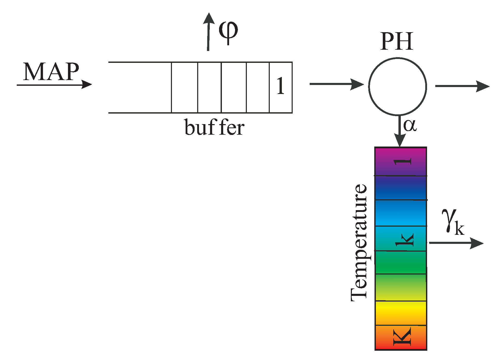
We consider a single-server queueing system that has an input buffer of an infinite capacity. Figure 1 illustrates the structure of the system under study.

Customer arrival is defined as the Markovian Arrival Process ($MAP$). Arrivals are governed by the underlying Markov chain ${\nu }_t,t\ge 0,$ with the finite state space $\left\{0,1,\dots ,W\}.\right.$ The residence time of this chain in the state $\nu$ has an exponential distribution with the parameter ${\lambda }_{\nu },\nu =\overline{0,W}.$ Here and in what follows, the notation $\nu =\overline{0,W}$ means that the integer parameter $\nu$ takes values from the set $\{0,1,\dots ,W\}.$ When the residence time in the state $\nu$ expires, with probability $p_{\nu ,{\nu }^{\prime }}\left(0\right)$, the process ${\nu }_t$ makes a transition to the state ${\nu }^{\prime }$ without generation of a customer, ${\nu }^{\prime }=\overline{0,W}\nu \ne {\nu }^{\prime },$ and, with probability $p_{\nu ,{\nu }^{\prime }}\left(1\right)$, the process ${\nu }_t$ makes a transition to the state ${\nu }^{\prime }$ with a generation of a customer, $\nu ,{\nu }^{\prime }=\overline{0,W}.$ The behavior of this arrival process is completely defined by the matrices $D_0$ and $D_1$ consisting of the entries ${\left(D_1\right)}_{\nu ,{\nu }^{\prime }}={\lambda }_{\nu }{p}_{\nu ,{\nu }^{\prime }}\left(1\right),\nu ,{\nu }^{\prime }=\overline{0,W,}$ and ${\left(D_0\right)}_{\nu ,\nu }=-{\lambda }_{\nu },\nu =\overline{0,W},{\left(D_0\right)}_{\nu ,{\nu }^{\prime }}={\lambda }_{\nu }{p}_{\nu ,{\nu }^{\prime }}\left(0\right),\nu ,{\nu }^{\prime }=\overline{0,W},\nu \ne {\nu }^{\prime }.$ The matrix $D\left(1\right)=D_0+D_1$ is assumed to be irreducible and is the generator of the process ${\nu }_t,t\ge 0$.

The mean arrival rate $\lambda$ is computes as $\lambda =\mathit{\theta }{D}_1\mathbf{e}$ where $\mathit{\theta }$ is the unique solution to the equations $\mathit{\theta }D\left(1\right)=\mathbf{0},\mathit{\theta }\mathbf{e}=1.$ Hereinafter, $\mathbf{e}$ denotes a column vector consisting of 1’s, and $\mathbf{0}$ is a zero row vector.

For more information about the $MAP$ and its properties, see [10,11,12].

The service time of a customer has a $PH$ distribution defined by the stochastic row vector $\mathit{\beta }$ and sub-generator $S.$ This time has the following interpretation. Let $m_t,t\ge 0,$ be the continuous-time Markov process having a finite state space $\{1,\dots ,M,M+1\}.$ The states $\{1,\dots ,M\}$ are transient and $M+1$ is the absorbing state. The initial state of this process at the moment of beginning of $PH$ distributed time is randomly selected among the transient states $\{1,\dots ,M\}$ according to the distribution defined by the entries of the row vector $\mathit{\beta }=({\beta }_1,\dots ,{\beta }_M)$. Then, the process $m_t$ makes transitions within the set $\{1,\dots ,M\}$ of the transient states with intensities defined by the entries of the sub-generator S or to the absorbing state. The intensities of the transition to the absorbing state are given by the entries of the column vector ${\mathit{S}}_0=-S\mathbf{e}.$ Transition to the absorbing state implies the end of $PH$ distributed time.

The Laplace–Stieltjes transform of the $PH$ distribution is defined as $\mathit{\beta }{(sI-S)}^{-1}{\mathit{S}}_0,Res>0.$ The mean service time is equal to $b_1=\mathit{\beta }{(-S)}^{-1}\mathbf{e}.$ For more detailed information about the $PH$ distribution, see [13]. Its applicability for good approximation of an arbitrary distribution is mentioned, e.g., in [14]. When the server becomes idle, the underlying process $m_t,t\ge 0,$ does not make any transitions.

The problem of constructing the vector $\mathit{\beta }$ and the matrices $D_0$ and $D_1,S$ based on available statistics regarding the real arrival and service processes is extensively addressed in the existing literature and may be solved following the results from, e.g., the papers [15,16,17].

During service, the server generates the heat and the temperature of the server is permanently monitored. Without essential loss of generality, we suppose that the temperature of the server is graded in some discrete units, e.g. degrees Celsius. The server can operate when this temperature is in the interval from $K^{\prime }$ to $K^{″}$. According to the 2011 version of recommendations of the American Society of Heating, Refrigerating and Air Conditioning Engineers (ASHRAE), for class A1 systems the temperature of the server has to be in the range from 15 ${}^{\circ }$C to 32 ${}^{\circ }$C. To simplify notations, we do not keep track of the absolute temperature of the server, but the excess of the temperature over the lower temperature level. This means that we assume that the (relative) temperature of the server has to be in the range from 0 to K where $K=K^{″}-K^{\prime }$. When the temperature of the server reaches the upper level K, service of customers becomes impossible. We say that this server becomes overheated. The server temporarily stops its work, is considered blocked and has to be cooled. A customer using the service when overheating occurs is assumed to be lost. We suggest that the server does not generate the heat when it does not work (is idle or blocked). When the server is working, the rate of the server heating is assumed to be equal to $\alpha$ degrees during unit of time, $\alpha >0.$ In parallel to heating of the server, it is permanently cooled. We assume that the cooling rate is equal to ${\gamma }_k,{\gamma }_k\ge 0,$ when the current temperature of the server is equal to $k,k=\overline{0,K}.$

When the server becomes overheated, it stops generation of the heat and only is cooled. We assume that the server remains blocked until its temperature drops to the level (threshold) $K_1,K_1<K.$ After that, the server becomes unblocked and can start service. We assume that the customers residing in the buffer are impatient. Each of these customers departs from the buffer without receiving service (is lost) independently of other waiting customers after a “patience time” expires. This time is exponentially distributed with the parameter $\varphi .$

The overheating of the server implies the loss of the potential profit gained by customers’ service. This loss is related to the loss of customers, during service of which the overheating occurs, and the loss of a capacity (throughput) of the server spent on service of such customers. The overheating may require server recovery, not only cooling. Therefore, it is desirable to avoid the overheating. To prevent the overheating occurrence, it is reasonable to stop new services when the temperature of the server becomes pretty high. We assume that the threshold $K_2$ is fixed such that $K_1<K_2\le K.$ The server cannot start new services if its temperature is equal or greater than $K_2.$ However, the ongoing service continues. It cannot be interrupted unless the server becomes overheated, i.e., its temperature becomes equal to $K.$ If this service is successfully finished while the server does not become overheated, the server remains blocked and does not start new services until its temperature drops to $K_1.$

It is obvious that the values of performance indicators of the system depend on the choice of the pair of thresholds $(K_1,K_2)$ and our first goal is to provide a way for computing the values of these measures for any fixed values of thresholds. To this end, we elaborate the algorithm for computation of the stationary distribution of the system states.

3. Process of System States and Its Analysis

Let the critical temperature K and thresholds $K_1$ and $K_2$ be fixed, $0\le K_1<K_2\le K.$

It is easy to see that the behavior of the considered system can be described by the following regular irreducible continuous-time Markov chain

$${\xi }_t=\{n_t,r_t,k_t,{\nu }_t,m_t\},t\ge 0,$$

where, during the epoch $t,t\ge 0,$

• $n_t$ is the number of customers in the buffer, $n_t\ge 0.$
• $r_t,r_t=\overline{0,2},$ is the server state: $r_t=0$ if the server is idle, $r_t=1$ if the server is busy, and $r_t=2$ if the server is blocked.
• $k_t$ is the temperature of the server, $k_t=\overline{0,K}.$
• ${\nu }_t$ is the state of the underlying process of the $MAP$, ${\nu }_t=\overline{0,W}.$
• $m_t$ is the state of the underlying process of the $PH$ service process, $m_t=\overline{1,M}.$

The Markov chain ${\xi }_t,t\ge 0,$ has the following state space:

$$\begin{array}{c}(\{0,0,k,\nu \},k=\overline{0,K_2-1})\bigcup (\{n,1,k,\nu ,m\},n\ge 0,k=\overline{0,K-1},m=\overline{1,M})\bigcup \\ (\{n,2,k,\nu \},n\ge 0,k=\overline{K_1+1,K}),\nu =\overline{0,W}.\end{array}$$

To formally define the Markov chain ${\xi }_t,$ we need to specify its transition rates within this state space. Since this chain has five components when the server is not idle or blocked and four components when the server is idle or blocked, to avoid operations with multi-dimensional arrays, it is necessary to enumerate the states in some order. We assume the lexicographic ordering. This means that firstly the states of the Markov chain ${\xi }_t$ are numbered in the increasing order of the component $n_t.$ Within the set of the states having the same value, say n, $n\ge 0,$ of this component, the states are numbered in the increasing order of the component $r_t.$ Within the set of the states having the same values, say $(n,r)$, $n\ge 0,r=0,1,2,$ of these components, the states are numbered in the increasing order of the component $k_t.$ Within the set of the states having the same values, say $(n,r,k),$$n\ge 0,r=0,1,2,k=\overline{0,K},$ of the three components, the states are numbered in the increasing order of the component ${\nu }_t,{\nu }_t=\overline{0,W}.$ Finally, the states from the sets $(n,1,k,\nu )$ are numbered in the increasing order of the component $m_t,m_t=\overline{1,M}.$

Let us denote by G the generator of the Markov chain ${\xi }_t.$ It follows from the introduced enumeration of the components of the chain that G is the matrix consisting of the blocks $G_{n,n^{\prime }},n,n^{\prime }\ge 0,$$|n-n^{\prime }|\le 1,$ defining the intensities of transitions from the states having the value n of the component $n_t$ to the states having the value $n^{\prime }$ of this component.

Theorem 1.

The infinitesimal generator G of the Markov chain ${\xi }_t,t\ge 0,$ has the following block-tridiagonal structure:

$$G=\left(\begin{array}{cccccc}{G}_{0,0}& G_{0,1}& O& O& O& \dots \\ G_{1,0}& G_{1,1}& G_{1,2}& O& O& \dots \\ O& G_{2,1}& G_{2,2}& G_{2,3}& O& \dots \\ ⋮& ⋮& ⋮& ⋮& ⋮& \ddots \end{array}\right).$$

Here, the blocks ${\left(G_{0,0}^{r,r^{\prime }}\right)}_{r,r^{\prime }=\overline{0,2}}$ of the matrix $G_{0,0},$ whose diagonal entries are negative and define, up to the sign, the intensities of the exit of the Markov chain ${\xi }_t$ from the corresponding states and the non-diagonal entries define the intensities of transitions that do not imply customers appearance in the empty buffer, have the following form:

$$G_{0,0}^{0,0}=I_{K_2}\otimes D_0+(E_{K_2}^{-}-C_{K_2})\otimes I_{\overline{W}},$$

$$G_{0,0}^{0,1}=I_{K_2,K}\otimes D_1\otimes \mathit{\beta },$$

$$G_{0,0}^{0,2}=O_{K_2\overline{W},(K-K_1)\overline{W}},$$

$$G_{0,0}^{1,0}=I_{K,K_2}\otimes I_{\overline{W}}\otimes {\mathbf{S}}_0,$$

$$G_{0,0}^{1,1}=I_K\otimes D_0\oplus S+(E_K^{-}-C_K+\alpha (E^{+}-I_K))\otimes I_{\overline{W}M},$$

$$G_{0,0}^{1,2}={\overline{I}}_{K,K-K_1}\otimes I_{\overline{W}}\otimes {\mathbf{S}}_0+\alpha \widehat{I}\otimes I_{\overline{W}}\otimes {\mathbf{e}}_M,$$

$$G_{0,0}^{2,0}={\gamma }_{K_1+1}{\tilde{I}}_{K-K_1,K_2}\otimes I_{\overline{W}},$$

$$G_{0,0}^{2,1}=O_{(K-K_1)\overline{W},K\overline{W}M},$$

$$G_{0,0}^{2,2}=I_{K-K_1}\otimes D_0+(\tilde{E}-\tilde{C})\otimes I_{\overline{W}}.$$

The matrix $G_{0,1},$ whose entries define the intensities of transitions when a customer arrives to the empty buffer, has the form

$$G_{0,1}=\left(\begin{array}{cc}{O}_{K_2\overline{W},K\overline{W}M}& O_{K_2\overline{W},(K-K_1)\overline{W}}\\ G_{0,1}^{1,1}& O_{K\overline{W}M,(K-K_1)\overline{W}}\\ O_{(K-K_1)\overline{W},K\overline{W}M}& G_{0,1}^{2,2}\end{array}\right)$$

where

$$G_{0,1}^{1,1}=I_K\otimes D_1\otimes I_M,$$

$$G_{0,1}^{2,2}=I_{K-K_1}\otimes D_1.$$

The matrix $G_{1,0},$ whose entries define the intensities of transitions when the single customer staying in the buffer, departs from the buffer (due to the impatience or service beginning), has the form

$$G_{1,0}=\left(\begin{array}{ccc}{O}_{K\overline{W}M,K_2\overline{W}}& G_{1,0}^{1,1}& O_{(K-K_1)\overline{W},K_2\overline{W}}\\ O_{(K-K_1)\overline{W},K_2\overline{W}}& G_{1,0}^{2,1}& G_{1,0}^{2,2}\end{array}\right),$$

where

$$G_{1,0}^{1,1}=\varphi I_{K\overline{W}M}+B\otimes I_{\overline{W}}\otimes {\mathbf{S}}_0\mathit{\beta },$$

$$G_{1,0}^{2,1}={\gamma }_{K_1+1}{\tilde{I}}_{K-K_1,K}\otimes I_{\overline{W}}\otimes \mathit{\beta },$$

$$G_{1,0}^{2,2}=\varphi I_{(K-K_1)\overline{W}}.$$

The blocks ${\left(G_{n,n}^{r,r^{\prime }}\right)}_{r,r^{\prime }=\overline{1,2}}$ of the matrix $G_{n,n},n\ge 1,$ whose diagonal entries are negative and define, up to the sign, the intensities of the exit of the Markov chain ${\xi }_t$ from the corresponding states when the number of customers in the buffer is equal to $n,n\ge 1,$ and the non-diagonal entries define the intensities of transitions that do not imply the change of the number of customers in the buffer, have the following form:

$$G_{n,n}^{1,1}=I_K\otimes D_0\oplus S+(E_K^{-}-C_K+\alpha (E^{+}-I_K)-n\varphi I_K)\otimes I_{\overline{W}M},$$

$$G_{n,n}^{1,2}={\overline{I}}_{K,K-K_1}\otimes I_{\overline{W}}\otimes {\mathbf{S}}_0+\alpha \widehat{I}\otimes I_{\overline{W}}\otimes {\mathbf{e}}_M,$$

$$G_{n,n}^{2,1}=O_{(K-K_1)\overline{W},K\overline{W}M},$$

$$G_{n,n}^{2,2}=I_{K-K_1}\otimes D_0+(\tilde{E}-\tilde{C})\otimes I_{\overline{W}}-n\varphi I_{(K-K_1)\overline{W}},n\ge 1.$$

The blocks ${\left(G_{n,n+1}^{r,r^{\prime }}\right)}_{r,r^{\prime }=\overline{1,2}}$ of the matrix $G_{n,n+1},n\ge 1,$ whose entries define the intensities of increasing the number of customers in the buffer from n to $n+1$, have the following form:

$$G_{n,n+1}^{1,1}=I_K\otimes D_1\otimes I_M,$$

$$G_{n,n+1}^{1,2}=O_{K\overline{W}M,(K-K_1)\overline{W}},$$

$$G_{n,n+1}^{2,1}=O_{(K-K_1)\overline{W},K\overline{W}M},$$

$$G_{n,n+1}^{2,2}=I_{K-K_1}\otimes D_1,n\ge 1.$$

The non-zero blocks ${\left(G_{n,n-1}^{r,r^{\prime }}\right)}_{r,r^{\prime }=\overline{1,2}}$ of the matrix $G_{n,n-1},n\ge 2,$ whose entries define the intensities of decreasing the number of customers in the buffer from n to $n-1$, have the following form:

$$G_{n,n-1}^{1,1}=n\varphi I_{K\overline{W}M}+B\otimes I_{\overline{W}}\otimes {\mathbf{S}}_0\mathit{\beta },$$

$$G_{n,n-1}^{2,1}={\gamma }_{K_1+1}{\tilde{I}}_{K-K_1,K}\otimes I_{\overline{W}}\otimes \mathit{\beta },$$

$$G_{n,n-1}^{2,2}=n\varphi I_{(K-K_1)\overline{W}},n\ge 2.$$

Here,

• I is the identity matrix, and O is a zero matrix of an appropriate dimension.
• $\overline{W}=W+1;$
• ⊗ and ⊕ are the symbols of the Kronecker product and the sum of matrices, respectively.
• $E_l^{-}$ is a square matrix of size l with all zero entries except the entries ${\left(E_l^{-}\right)}_{k,k-1}={\gamma }_k,k=\overline{1,l-1}$.
• $C_l$ is a square matrix of size l with all zero entries except the entries ${\left(C_l\right)}_{k,k}={\gamma }_k,k=\overline{1,l-1}$.
• $I_{K_2,K}$ is a matrix of size $K_2\times K$ with all zero entries except the entries ${\left(I_{K_2,K}\right)}_{n,n},n=\overline{0,K_2-1},$ which are equal to 1.
• $I_{K,K_2}$ is a matrix of size $K\times K_2$ with all zero entries except the entries ${\left(I_{K,K_2}\right)}_{n,n},n=\overline{0,K_2-1},$ which are equal to 1.
• $E^{+}$ is a square matrix of size K with all zero entries except the entries ${\left(E^{+}\right)}_{k,k+1},k=\overline{0,K-2},$ which are equal to 1.
• ${\overline{I}}_{K,K-K_1}$ is a matrix of size $K\times (K-K_1)$ with all zero entries except the entries ${\left({\overline{I}}_{K,K-K_1}\right)}_{n,n-K_1-1},n=\overline{K_2,K-1},$ which are equal to 1.
• $\widehat{I}$ is a matrix of size $K\times (K-K_1)$ with all zero entries except the entry ${(\widehat{I})}_{K-1,K-K_1-1},$ which is equal to 1.
• ${\tilde{I}}_{K-K_1,K_2}$ is a matrix of size $(K-K_1)\times K_2$ with all zero entries except the entry ${({\tilde{I}}_{K-K_1,K_2})}_{0,K_1},$ which is equal to 1.
• $\tilde{E}$ is a square matrix of size $K-K_1$ with all zero entries except the entries ${(\tilde{E})}_{k,k-1}={\gamma }_{K_1+k+1},k=\overline{1,K-K_1-1}$.
• $\tilde{C}$ is a square matrix of size $K-K_1$ with all zero entries except the entries ${(\tilde{C})}_{k,k}={\gamma }_{K_1+k+1},k=\overline{0,K-K_1-1}$.
• B is a square matrix of size K with all zero entries except the entries ${(B)}_{k,k}=1,k=\overline{0,K_2-1}$.
• ${\tilde{I}}_{K-K_1,K}$ is a matrix of size $(K-K_1)\times K$ with all zero entries except the entry ${({\tilde{I}}_{K-K_1,K})}_{0,K_1}=1$.

The proof of the theorem is implemented via the careful analysis of various scenarios of the system behavior at the moments of changing the states of the underlying processes of arrivals and service, changing the temperature of the server due to heating and cooling, customers departure due to impatience. The symbols of Kronecker product and sum of matrices are very helpful for description of transition intensities of several independent Markov processes.

It can be easily shown that the Markov chain ${\xi }_t$ belongs to the class of Asymptotically Quasi–Toeplitz Markov Chains ($AQTMC$) (see [2]).

Theorem 2.

The stationary distribution of the Markov chain ${\xi }_t$ exists for any values of the system parameters.

The assertion of the theorem stems from the fact that the customers staying in the buffer are assumed to be impatient ($\varphi >0$). The strict proof of Theorem 2 can be done by using the results from [2]. This proof is straightforward and rather routine, thus it is omitted here.

Let us denote by $\mathit{\pi }(n,r,k)$ the row vector of stationary probabilities of the states of the chain having the value $(n,r,k)$ of the first three components listed in the described above order.

In addition, denote

$$\mathit{\pi }(0,0)=(\mathit{\pi }(0,0,0),\dots ,\mathit{\pi }(0,0,K_2-1)),$$

$$\mathit{\pi }(n,1)=\left(\mathit{\pi }\right(n,1,0),\dots ,\mathit{\pi }(n,1,K-1\left)\right),$$

$$\mathit{\pi }(n,2)=(\mathit{\pi }(n,2,K_1+1),\dots ,\mathit{\pi }(n,2,K)),n\ge 0,$$

$$\mathit{\pi }\left(0\right)=\left(\mathit{\pi }\right(0,0),\mathit{\pi }(0,1),\mathit{\pi }(0,2\left)\right),\mathit{\pi }\left(n\right)=\left(\mathit{\pi }\right(n,1),\mathit{\pi }(n,2\left)\right),n\ge 1.$$

Because the state space of the Markov chain ${\xi }_t$ is infinite and the generator G of this chain does not have Toeplitz-like structure, the problem of computation of the vectors $\mathit{\pi }\left(n\right),n\ge 0,$ is not easy. Fortunately, the chains with the generator of such a type were analysed in [2,3] and the algorithms developed in those papers allow computing these vectors.

4. Performance Indicators

Once the vectors $\mathit{\pi }\left(n\right),n\ge 0,$ have been computed, we can calculate various performance indicators of the system.

The mean number N of customers in the buffer is computed by

$$N=\sum _{n=1}^{\infty }n\mathit{\pi }\left(n\right)\mathbf{e}.$$

The average temperature T of the server is computed by

$$T=\sum _{k=1}^{K_2-1}k\mathit{\pi }(0,0,k)\mathbf{e}+\sum _{n=0}^{\infty }\sum _{k=1}^{K-1}k\mathit{\pi }(n,1,k)\mathbf{e}+\sum _{n=0}^{\infty }\sum _{k=K_1+1}^{K}k\mathit{\pi }(n,2,k)\mathbf{e}.$$

The variance of the temperature of the server is equal to

$$\sum _{k=1}^{K_2-1}{k}^2\mathit{\pi }(0,0,k)\mathbf{e}+\sum _{n=0}^{\infty }\sum _{k=1}^{K-1}{k}^2\mathit{\pi }(n,1,k)\mathbf{e}+\sum _{n=0}^{\infty }\sum _{k=K_1+1}^K{k}^2\mathit{\pi }(n,2,k)\mathbf{e}-T^2.$$

The probability $P_{idle}$ that the server is idle at an arbitrary moment is

$$P_{idle}=\mathit{\pi }(0,0)\mathbf{e}.$$

The probability $P_{imm}$ that the server is idle at the moment of an arbitrary customer arrival (and this customer immediately starts service) is

$$P_{imm}=\frac{1}{\lambda }\mathit{\pi }(0,0)(I_{K_2}\otimes D_1)\mathbf{e}.$$

The probability $P_{busy}$ that the server is busy at an arbitrary moment is

$$P_{busy}=\sum _{n=0}^{\infty }\mathit{\pi }(n,1)\mathbf{e}.$$

The average number $N_{system}$ of customers in the system is computed by $N_{system}=N+P_{busy}.$

The probability $P_{block}$ that the server is blocked at an arbitrary moment is

$$P_{block}=\sum _{n=0}^{\infty }\mathit{\pi }(n,2)\mathbf{e}.$$

The probability $P_{imp}$ of an arbitrary customer loss due to impatience is

$$P_{imp}=\frac{\varphi N}{\lambda }.$$

The intensity ${\lambda }_{out}$ of the flow of served customers is

$${\lambda }_{out}=\sum _{n=0}^{\infty }\mathit{\pi }(n,1)({\mathbf{e}}_{K\overline{W}}\otimes {\mathbf{S}}_0).$$

The probability $P_{overheating}$ of an arbitrary customer loss due to the server overheating is

$$P_{overheating}=\alpha {\lambda }^{-1}\sum _{n=0}^{\infty }\mathit{\pi }(n,1,K-1)\mathbf{e}.$$

The intensity $l_{vacation}$ of the transition after the service completion to the vacation regime (the server is overheated or is preventively switched-off for cooling) is

$$l_{vacation}=\sum _{n=0}^{\infty }\mathit{\pi }(n,1)({\overline{I}}_{K,K-K_1}\otimes I_{\overline{W}}\otimes {\mathbf{S}}_0)\mathbf{e}.$$

The probability $P_{loss}$ of an arbitrary customer loss is computed as

$$P_{loss}=P_{imp}+P_{overheating}=1-\frac{{\lambda }_{out}}{\lambda }.$$

5. Numerical Example

Let the $MAP$ arrival flow be defined by the matrices

$$D_0=\left(\begin{array}{cc}-0.3379101412& 0\\ 0& -0.0109675577\end{array}\right),D_1=\left(\begin{array}{cc}0.3356635104& 0.0022466308\\ 0.0061087109& 0.0048588468\end{array}\right).$$

The mean arrival rate is $\lambda =5,$ the coefficient of correlation of two successive intervals between arrivals $c_{cor}=0.2,$ and the squared coefficient of variation of these intervals $c_{var}=12.4.$

Let the maximum value of the temperature be $K=50,$ and the rate of the heat generation be $\alpha =1.$ The rate of the server cooling when its temperature is equal to k is ${\gamma }_k=\frac{0.3k}{K},k=\overline{1,K-1},$${\gamma }_K=0.01.$

The rate of a customer departure from the buffer due to impatience is $\varphi =0.0015.$

The service time of a customer has the $PH$ distribution with the irreducible representation $(\mathit{\beta },S)$ where $\mathit{\beta }=(0.9,0.1),$ $S=\left(\begin{array}{cc}-6& 0\\ 0& -0.2\end{array}\right).$ The average service time is equal to 0.65 and the squared coefficient of variation of the service time is equal to 10.95.

Let us vary the threshold $K_1$ over the interval $[0,K)$ and the parameter $K_2$ over the interval $[K_1+1,K].$

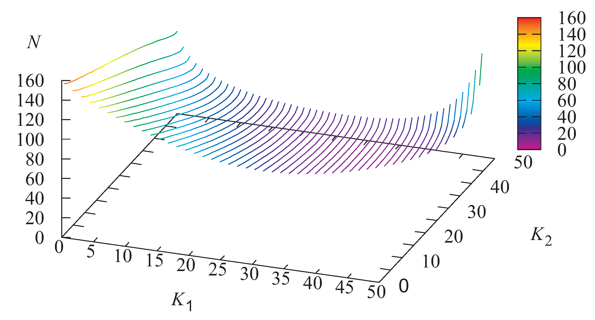
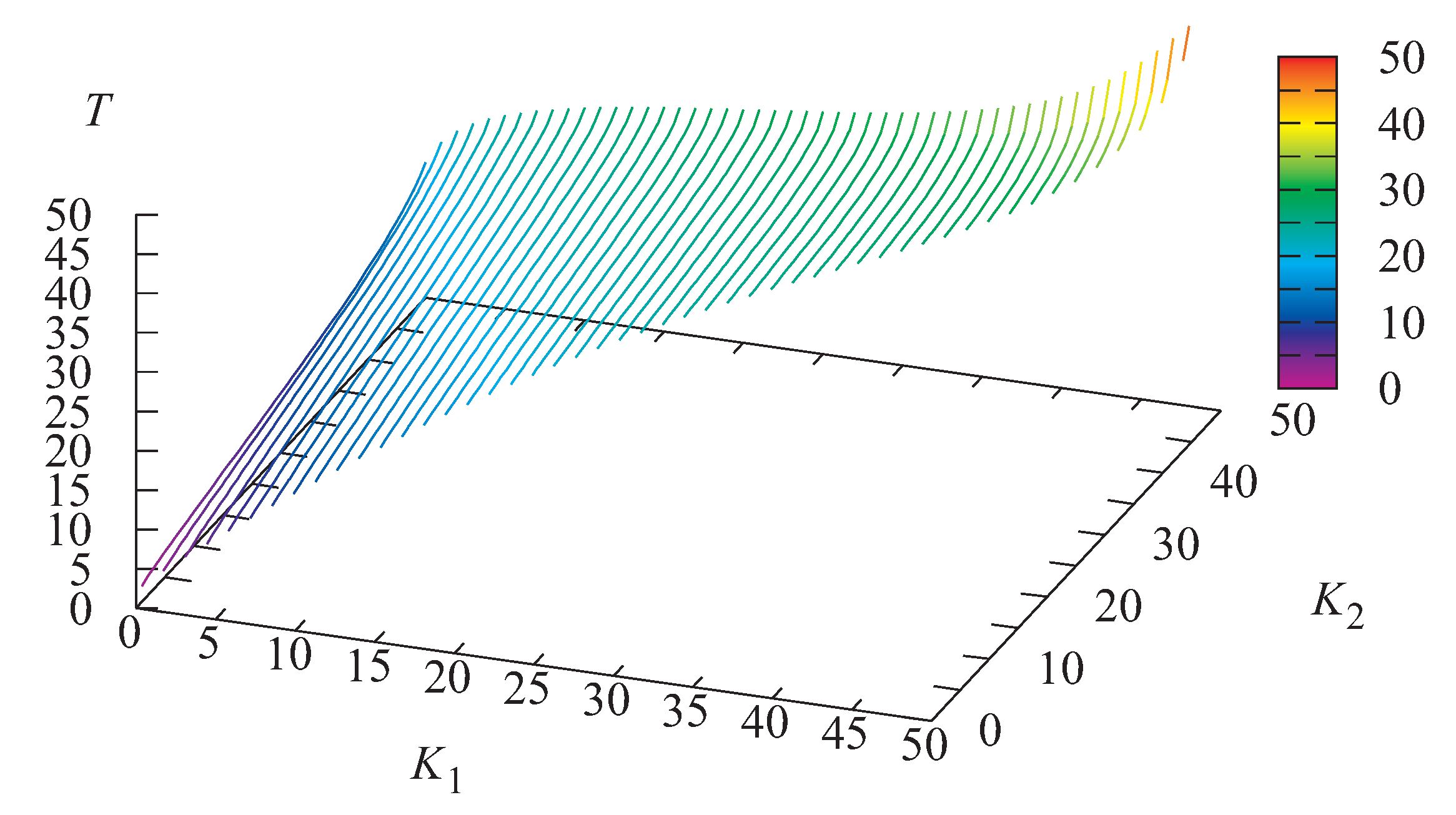
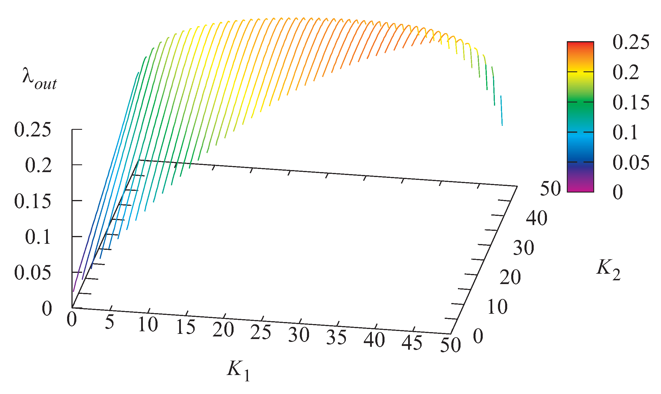
Figure 2, Figure 3 and Figure 4 illustrate the dependence of the average number N of customers in the buffer, the average intensity ${\lambda }_{out}$ of the flow of served customers and the average temperature T of the server on the values of $K_1$ and $K_2.$

It can be observed in Figure 2 that the average number N of customers in the buffer increases when the threshold $K_2$ grows. This is easily explained by the fact that the probability of overheating occurrence increases when the threshold $K_2$ becomes close to the critical temperature. It is assumed that the rate of the server cooling is small after overheating occurrence, the blocking period of the server becomes large and a lot of customers stay in the buffer. It should be noted that, for any fixed value of $K_2$ there exists a value of $K_1$, which minimizes the average number N. The average intensity ${\lambda }_{out}$ of the flow of served customers is small when both thresholds $K_1$ and $K_2$ are small (low temperature of the server is guaranteed at expense of managing too long blocking periods) and when both thresholds $K_1$ and $K_2$ are large (the server is quite often overheated, which causes the corresponding loss of customers). This intensity ${\lambda }_{out}$ is much higher for intermediate values of the thresholds $K_1$ and $K_2.$ Figure 4 well matches to the just given explanation of the surface in Figure 3.

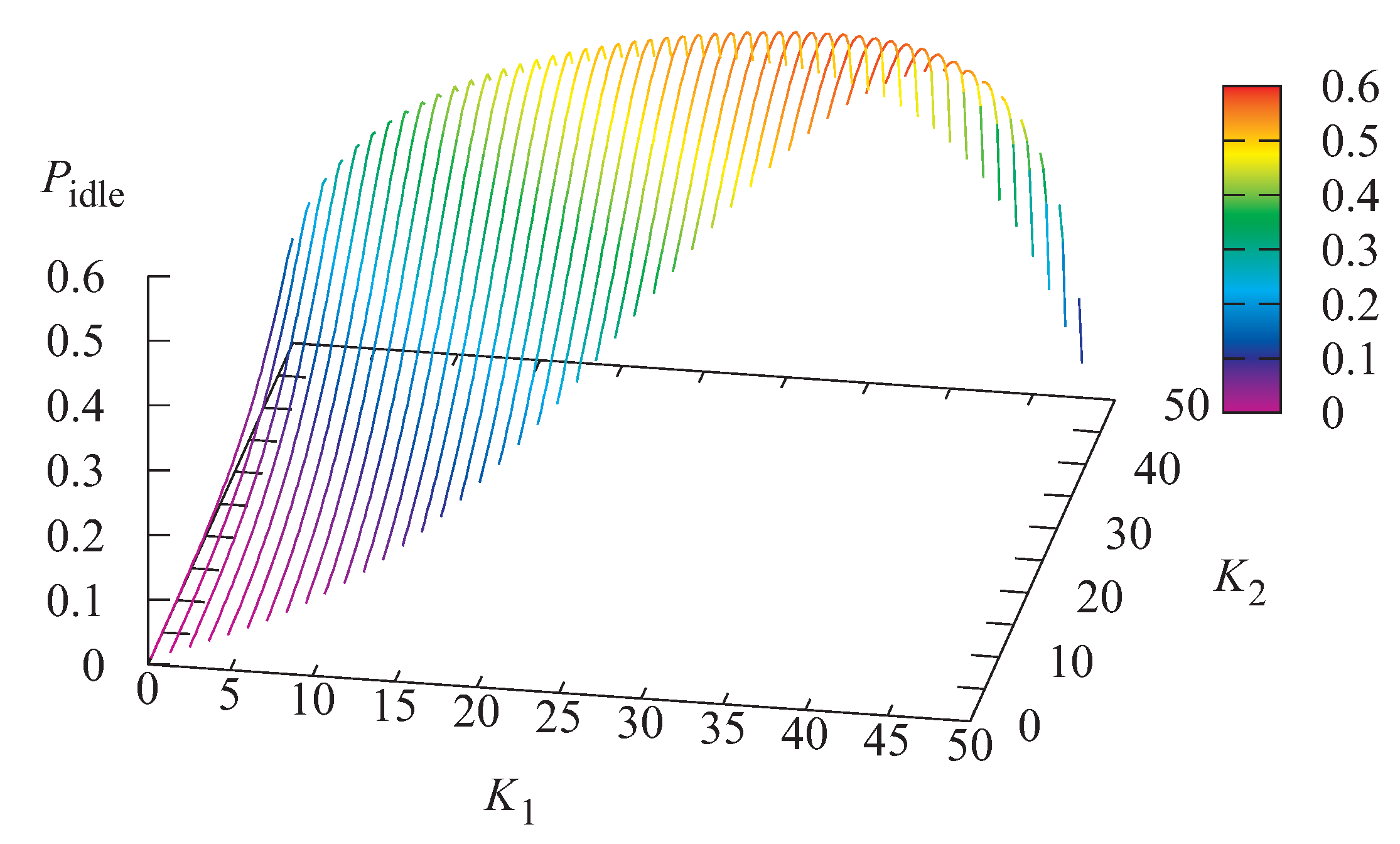
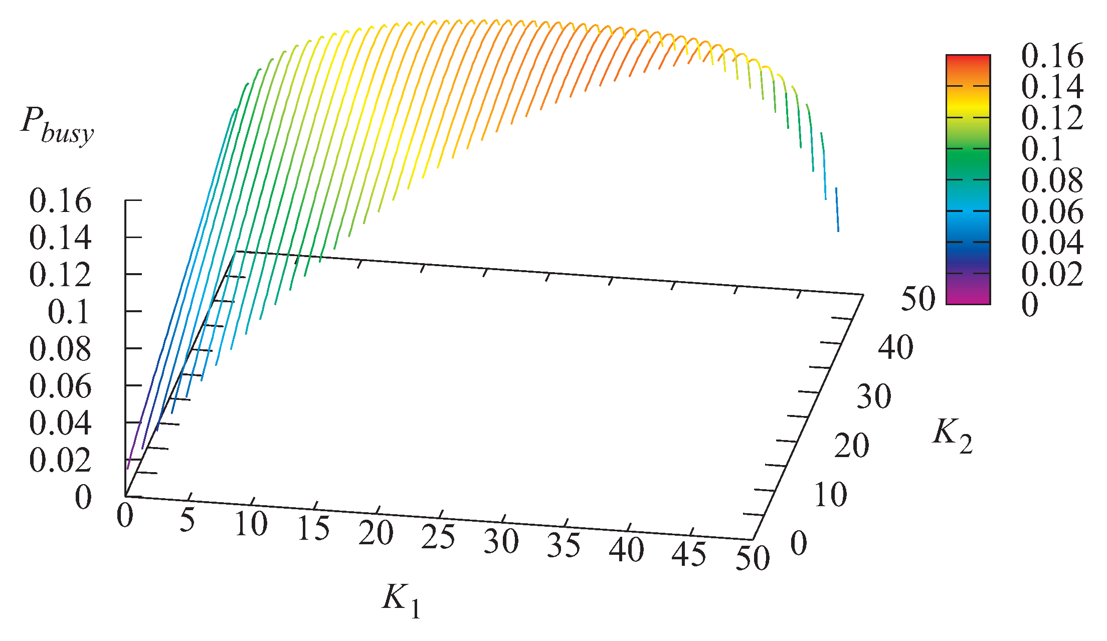
Figure 5, Figure 6 and Figure 7 illustrate the dependence of the probability $P_{idle}$ that the server is idle, the probability $P_{busy}$ that the server is busy, and the probability $P_{block}$ that the server is blocked at an arbitrary moment on the values of $K_1$ and $K_2.$

The probability $P_{idle}$ that the server is idle and the probability $P_{busy}$ that the server is busy also are maximal for intermediate values of thresholds $K_1$ and $K_2.$ As expected, the probability $P_{block}$ that the server is blocked decreases when the threshold $K_1$ grows.

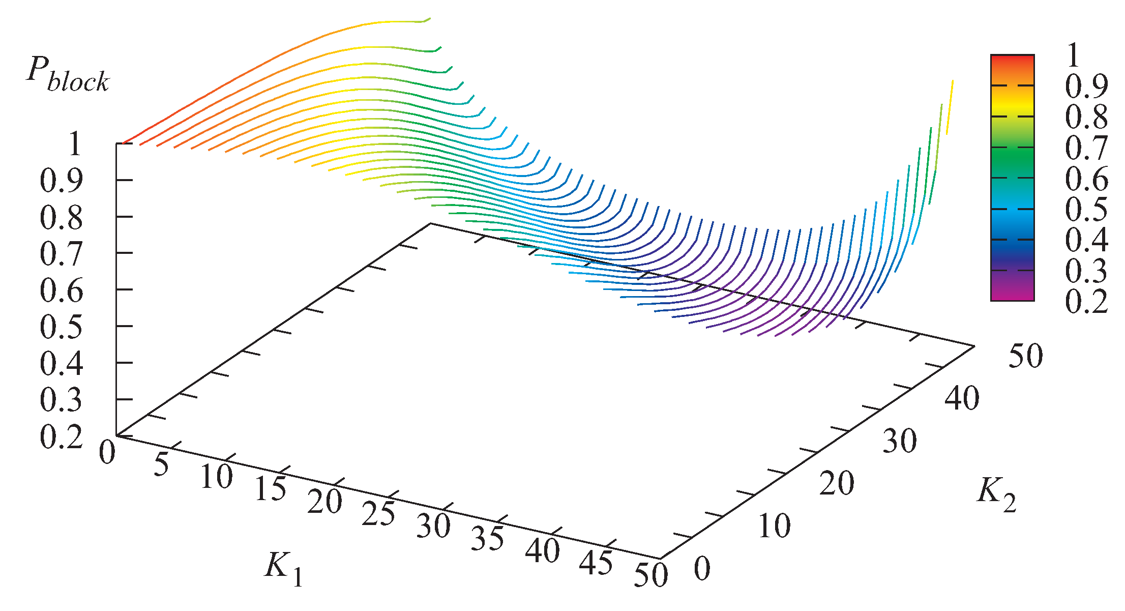
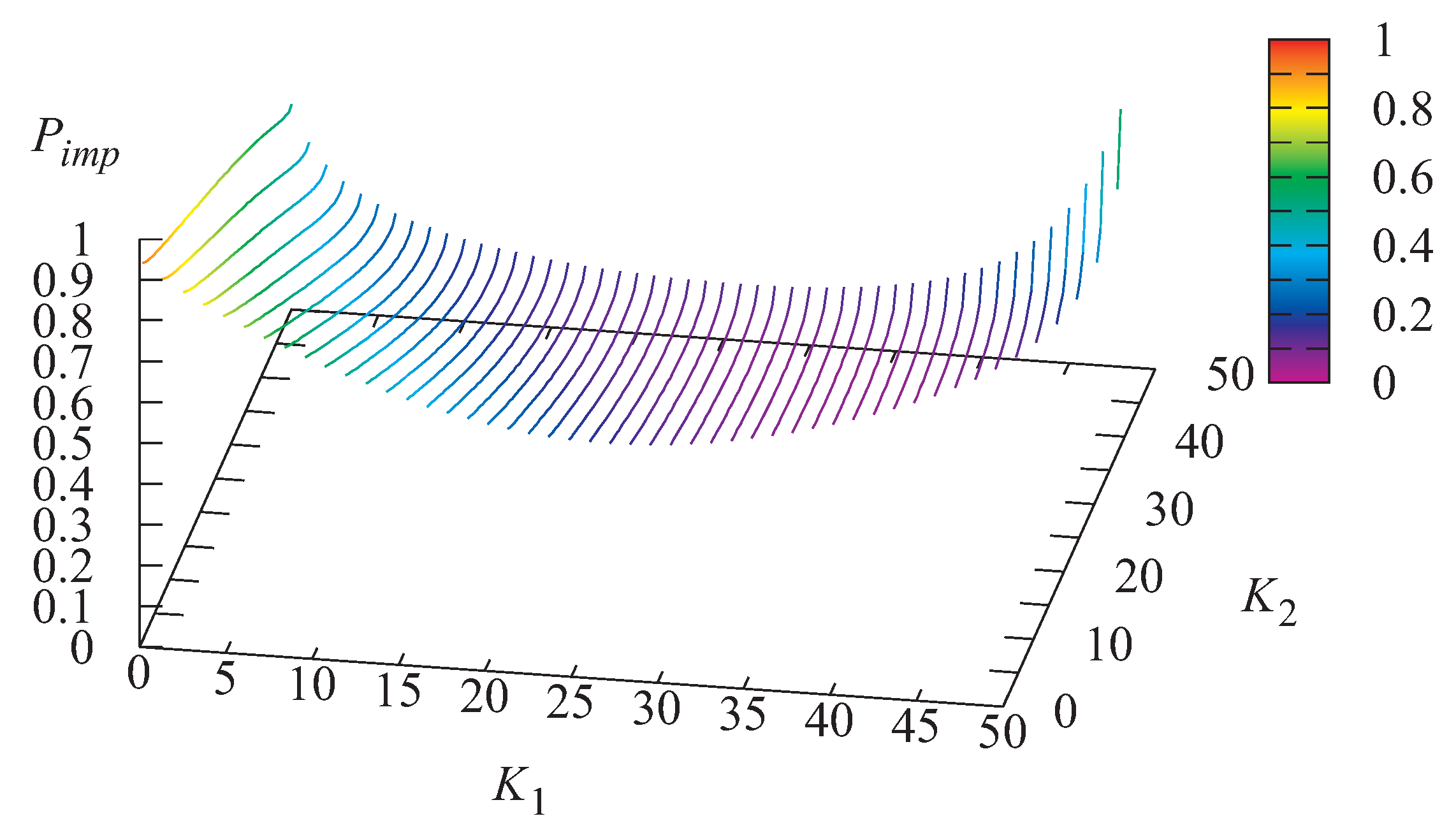
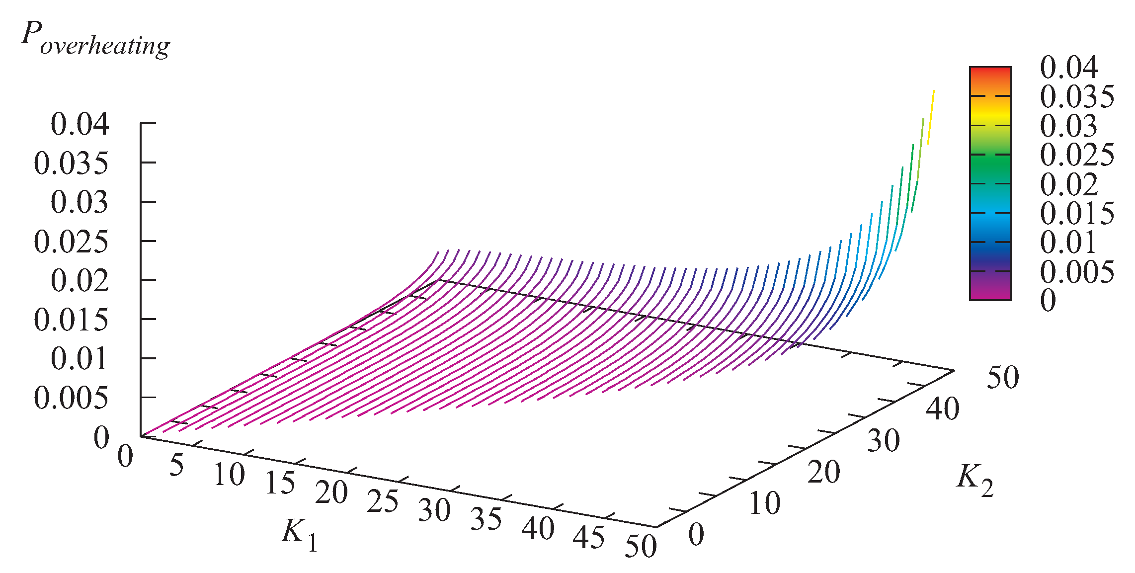
Figure 8, Figure 9 and Figure 10 illustrate the dependence of the probability $P_{imp}$ that an arbitrary customer is lost due to impatience, the loss probability $P_{overheating}$ that an arbitrary customer is lost due to server overheating, and the probability $P_{loss}$ that an arbitrary customer is lost on the values of $K_1$ and $K_2.$

Figure 9 evidently shows that the loss probability $P_{overheating}$ that an arbitrary customer is lost due to server overheating sharply increases when the thresholds $K_1$ and $K_2$ grow. Therefore, the proposed mechanism for preventing overheating is highly effective. It can be observed in Figure 8, Figure 9 and Figure 10 that there exists a pair of the thresholds that minimizes the loss probability $P_{loss}.$ The minimal value of the probability $P_{loss}$ in this example is equal to 0.065255 and is achieved under the following values of the thresholds: $K_1=36$ and $K_2=37.$

Customers loss in the considered system occurs due to overheating of the server during ongoing service and due to impatience of customers. The charges paid for these types of losses may be different. The charge paid for the loss due to overheating can be much higher because the loss due to impatience is just the loss of potential profit, while the loss due to overheating means the real loss of a customer, violation of service level agreement and possible expenditures to return the overheated server to the operable mode. Therefore, various other optimization problems can be formulated.

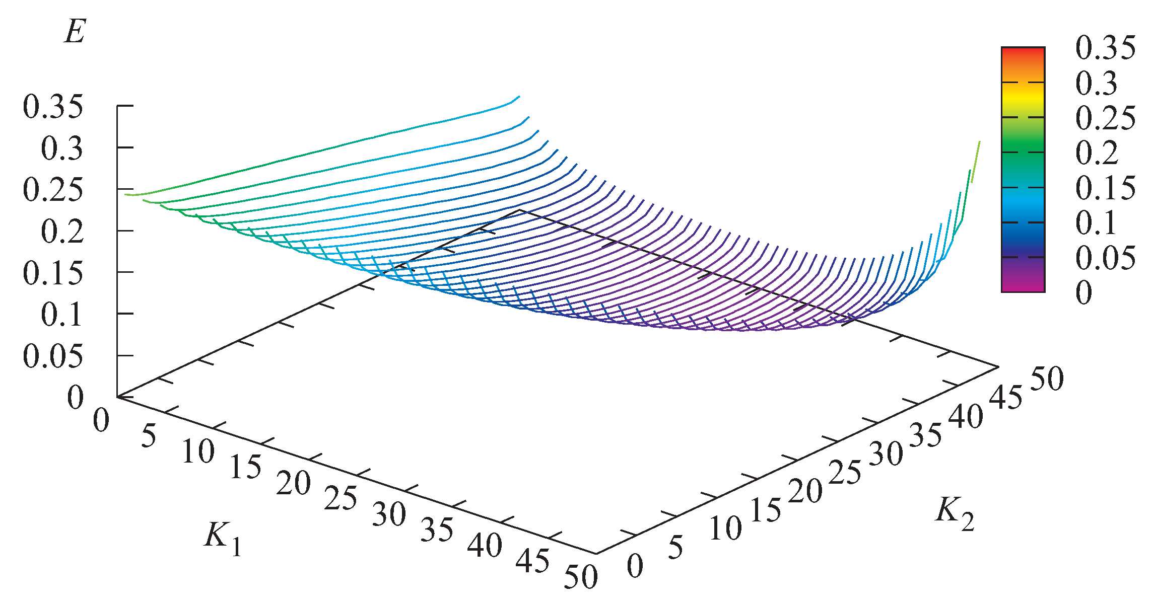
In this paper, we consider the following economical criterion of the quality of the system operation:

$$E=a\lambda P_{imp}+(b+c)\lambda P_{overheating}+c{l}_{vacation}.$$

This economical criterion indicates the charge paid by the system per unit of time, where a is the charge paid by the system for each customer loss due to impatience, b is the charge paid by the system for customer loss due to overheating, and c is the charge paid by the system for managing operation of the system via each transition to the blocking regime.

Let us fix the following values of the cost coefficients: $a=1,b=10,c=2.$

Figure 11 illustrates the dependence of the economical criterion E on the values of $K_1$ and $K_2.$

The minimal value of the economical criterion E here is equal to $E^{\ast }=0.0308509$ and is achieved when $K_1=29$ and $K_2=42.$ Note that, for the same system but without control, when no prevention of overheating is assumed (i.e., $K_2=50$, indicating the server is switched-off only when it becomes overheated, and $K_1=49$), the value of the economical criterion is more than ten times higher: $E(49,50)=0.309677.$

6. Conclusions

In this paper, a novel in the literature queueing model is considered. This model considers the possible heating of a server during the service process that causes the necessity of its permanent cooling. Such a model can be applied, e.g., for optimization of operation of servers of data centers that generate a lot of heat during their operation and the proper cooling mechanisms have to be used to avoid a collapse of the server. We offer the discipline for control by the system operation aiming to prevent premature overheating of a server and the loss of customers. This discipline is defined by two thresholds. One threshold is used to define the temperature of a server that when exceeded causes the stop of new services and to block the server when its temperature becomes close to the critical temperature. One more threshold is used to define the temperature when the blocking of the server can be finished and service can be resumed. The system is analyzed under quite general assumptions about the arrival and service processes. The generator of the multi-dimensional Markov chain, which describes the behavior of the system under any values of thresholds, is derived. This allows computing the stationary distribution of the states of the Markov chain and the key performance indicators of the system. Usefulness of the proposed strategy of preventive control is demonstrated via numerical experiments.

The obtained results can be used for managerial goals. In fact, the results can be used for the choice of the proper equipment for service provisioning (accounting for the different speeds of operation and heat generation by the different servers), its cooling and optimal management by periodical switching-off the server via the optimal choice of the thresholds.

As directions for future research, systems with the Batch Markov Arrival Process, phase-type distribution of heating and cooling times, several possible modes of the server operation (with various service and heating rates), etc., can be considered.