Numerical Solution of Heston-Hull-White Three-Dimensional PDE with a High Order FD Scheme

Abstract

A new numerical method for tackling the three-dimensional Heston–Hull–White partial differential equation (PDE) is proposed. This PDE has an application in pricing options when not only the asset price and the volatility but also the risk-free rate of interest are coming from stochastic nature. To solve this time-dependent three-dimensional PDE as efficiently as possible, high order adaptive finite difference (FD) methods are applied for the application of method of lines. It is derived that the new estimates have fourth order of convergence on non-uniform grids. In addition, it is proved that the overall procedure is conditionally time-stable. The results are upheld via several numerical tests.

1. Introduction

To model different types of derivatives in finance, a common approach is to investigate the connections of these factors to each other, formulated as a stochastic differential equation (SDEs). The factors could be the underlying asset, the volatility, domestic and foreign interest rates, etc., [1,2]. As such, the important action of pricing option under different payoffs can be modeled and simulated via the SDEs or their corresponding partial differential equation (PDE) formulation.

However, a frequently occurring issue is that whatever the model becomes complicated and more realistic, the procedure of having and representing its exact solution becomes harder, see, e.g., [3,4,5].

To discuss more and from the beginning, the classical model of Black–Scholes in pricing contracts does not cover and illustrate all the aspects of an option in a complete market, such as market risks, stochastic volatility (SV), and asymmetries seen in data of market, [6]. Some remedies to this well-known model are via non-lognormal hypothesis for a SDE, that indicates some modifications of the volatility and the underlying asset. We recall that Heston in [7] extended and improved the behavior of the Black–Scholes model by involving more risky factor into the model, i.e., by considering the volatility to be stochastic as well. Further discussions can be found at [6,8].

On the other hand, as long as the foreign exchange (FX) products are involved and a trader encounters a situation in which the interest rate is not anymore constant during the lifetime of an option, then investigating and proposing an improved model, having stochastic rates of interest, such as the power-reverse dual-currency and the Heston–Cox–Ingersoll–Ross (HCIR) problems (refer to [9] and the references therein for more background).

1.1. Problem Formulation

The option pricing problem under the 3D Heston–Hull–White (HHW) model as a PDE model is defined by [10]:

$$\begin{array}{c}\hfill \begin{array}{cc}\hfill \frac{\partial u(s,v,r,t)}{\partial t}=& \frac{1}{2}{s}^{2}v\frac{{\partial }^{2}u(s,v,r,t)}{\partial s^2}+\frac{1}{2}{\sigma }_1^{2}v\frac{{\partial }^{2}u(s,v,r,t)}{\partial v^2}+\frac{1}{2}{\sigma }_2^2\frac{{\partial }^{2}u(s,v,r,t)}{\partial r^2}\hfill \\ & +{\rho }_{12}{\sigma }_{1}sv\frac{{\partial }^{2}u(s,v,r,t)}{\partial s\partial v}+{\rho }_{13}{\sigma }_{2}s\sqrt{v}\frac{{\partial }^{2}u(s,v,r,t)}{\partial s\partial r}\hfill \\ & +{\rho }_{23}{\sigma }_1{\sigma }_2\sqrt{v}\frac{{\partial }^{2}u(s,v,r,t)}{\partial v\partial r}\hfill \\ & +rs\frac{\partial u(s,v,r,t)}{\partial s}+\kappa (\eta -v)\frac{\partial u(s,v,r,t)}{\partial v}\hfill \\ & +a(b(T-t)-r)\frac{\partial u(s,v,r,t)}{\partial r}\hfill \\ & -ru(s,v,r,t).\hfill \end{array}\end{array}$$

(1)

Here $\kappa >0$ shows the volatility adjustment speed to the analytical mean $\eta >0$, while ${\sigma }_1,{\sigma }_2,a$ are some parameters. In addition, the correlation parameters are ${\rho }_{12}$, ${\rho }_{13}$, ${\rho }_{23}\in [-1,1]$, b is a time function.

In pricing under call options, the (terminal/)initial condition is given by [11,12]:

$$u(s,v,r,0)={\left(s-E\right)}^{+},$$

(2)

where the strike price is E. In a similar way, for a put option, it is given as follows:

$$u(s,v,r,0)={\left(E-s\right)}^{+}.$$

(3)

As discussed in [13,14], the fair pricing procedure should be carried out by computational schemes since the corresponding high-dimensional PDEs, constructed for such options, do not admit any analytical or semi-analytical solutions, see [15,16] for further background.

1.2. Novelties and Motivation

The contribution of this article reads in proposing a solution method via an un-equally spaced grid having a focus on the hot area in option pricing under the HHW PDE problem. Studying and coding multi dimensional problems with discretization methods while the grid of points are non-uniform is a challenging and intensive task, but could clearly increase the accuracy of the approximate solution by applying fewer numbers of grid nodes in contrasts to the uniform discretization. This reduces the size of the discretized problem and is useful in practice.

To this aim, (1) is tackled by employing high order fourth-order finite difference approximations. We apply fourth order discretizations on a stencil having five and six non-equidistant nodes. Derivation and construction of fourth-order compact FD method for HHW PDE is new and useful in practice.

In fact, the method-of-lines technique is considered to build a set of ODEs with time-varying system matrix. All the side conditions are imposed therein as well. Thence, a method to march along time for the set of ODEs is provided in Section 3 and it is analytically illustrated that the presented numerical procedure is conditionally time-stable when b is not changing by time.

Recalling that here adaptive FD formulas are constructed to hit some features simultaneously, viz., to be effective, results in sparse operators and being able to handling non-uniform grids.

Motivated by recent works in this field (see e.g., [17]), we aim at proposing higher order schemes for the HHW equation on non-uniform meshes so as to increase the accuracy of obtained option prices without increasing the computational load so much. The novelties and contributions of our work are given below:

• We propose fourth-order adaptive discretizations for the spatial variables.
• The beauty of our scheme is the use of non-uniform grid of nodes with an adaptation on the hotzone.
• We provide a new stability bound for the resulting fully discretized set of equations when pricing under HHW PDE using high order discretization methods along the spatial as well as the temporal variables.

1.3. Grid Generation

The option pricing problem (1) is considered in the unbounded area

$$(s,v,r,t)\in \Omega \times (0,T],$$

(4)

wherein $\Omega =[0,+\infty )$$\times [0,+\infty )\times [0,+\infty )$. For tackling the financial model numerically, one can take into account the following domain [18]:

$$\Omega =[0,s_{max}]\times [0,v_{max}]\times [-r_{max},r_{max}],$$

(5)

wherein $s_{max}$, $v_{max}$, $r_{max}$ are three positive real constants and assumed to be large enough.

Since the PDE model is coercive (sometimes called degenerate) at $v=0$, its payoff is non-smooth at $s=E$, and the working domain has large width, thus it is requisite to use non-uniform meshes, at which the location of the nodes are not equally-spaced. This helps in producing results of higher accuracy with adapting to the hotzone of the problem.

Let ${\left\{s_i\right\}}_{i=1}^m$ be a set of non-uniform nodes along s as follows [13,19]:

$$s_i=\phi \left({\xi }_i\right),1\le i\le m,$$

(6)

where $m>1$ and ${\xi }_{min}={\xi }_1<{\xi }_2<\cdots <{\xi }_m={\xi }_{max}$ are m equi–distant points with the following characteristics: ${\xi }_{min}={sinh}^{-1}\left(\frac{s_{min}-s_{\mathrm{left}}}{d_1}\right)$, ${\xi }_{\mathrm{int}}=\frac{s_{\mathrm{right}}-s_{\mathrm{left}}}{d_1}$, ${\xi }_{max}={\xi }_{\mathrm{int}}+{sinh}^{-1}\left(\frac{s_{max}-s_{\mathrm{right}}}{d_1}\right)$, wherein $s_{min}=0$. Here $d_1>0$ controls the density of the nodes around $s=E$. We also have:

$$\phi \left(\xi \right)=\left\{\begin{array}{cc}{s}_{\mathrm{left}}+d_{1}sinh\left(\xi \right),\hfill & {\xi }_{min}\le \xi <0,\hfill \\ s_{\mathrm{left}}+d_1\xi ,\hfill & 0\le \xi \le {\xi }_{\mathrm{int}},\hfill \\ s_{\mathrm{right}}+d_{1}sinh(\xi -{\xi }_{\mathrm{int}}),\hfill & {\xi }_{\mathrm{int}}<\xi \le {\xi }_{max}.\hfill \end{array}\right.$$

(7)

Throughout this work, we used the same value for $d_1=\frac{E}{20}$ while $s_{\mathrm{left}}=max\{0.5,exp\{-0.25T\}\}\times E$, $[s_{\mathrm{left}},s_{\mathrm{right}}]\subset [0,s_{max}]$, $s_{\mathrm{right}}=E$ and $s_{max}=14E$.

The nodes along v, i.e., ${\left\{v_j\right\}}_{j=1}^n$ are defined by:

$$v_j=d_{2}sinh\left({\varsigma }_j\right),1\le j\le n,$$

(8)

where $d_2>0$ gives the concentration around $v=0$. In this work, we used $d_2=\frac{v_{max}}{500}$, where $v_{max}=10$. In addition, ${\varsigma }_j$ are equally spaced points given by:

$${\varsigma }_j=(j-1)\Delta \varsigma ,\Delta \varsigma =\frac{1}{n-1}{sinh}^{-1}\left(\frac{v_{max}}{d_2}\right),$$

(9)

for any $1\le j\le n$. The non-uniform nodes along r are defined as follows:

$$r_k=d_{3}sinh\left({\zeta }_k\right),1\le k\le o,$$

(10)

whereas $d_3=\frac{r_{max}}{500}$ is a positive parameter and $r_{max}=1$. We also have ${\zeta }_k=(k-1)\Delta \zeta$, $\Delta \zeta =\frac{1}{o-1}{sinh}^{-1}\left(\frac{r_{max}}{d_3}\right)$. Note that denser mesh points in the important area could circumvent the problems happening in solving (1), like non-smoothness of payoffs (2) and (3) at $s=E$, and the degeneracy at $v=r=0$.

We state that a detailed study into possibly better choices for the involved parameters in mesh generating may be interesting, but this is beyond the scope of the current research. Furthermore, the non-smoothness arising in the payoff would ruin the convergence rate of most derivative approximation particularly on uniform meshes and due to this, the application of non-uniform nodes is indispensable for efficient numerical solution of (1).

1.4. Manuscript Organization

The remaining parts of this work are organized as follows. In Section 2, the weights of the FD scheme over non-uniform grids (here we also call adaptive grids with special emphasis on the hot zone) are derived to attain the higher rate of convergence four.

Section 3 is devoted to the application of a sixth order Runge–Kutta time stepping method to advance along time when semi-discretize the HHW PDE. We prove that the new procedure is time-stable conditionally based on the largest eigenvalue of the system matrix. Section 4 shows that numerical performances are more useful than the earlier schemes with quicker convergence behavior. Finally, some conclusions are drawn in Section 5.

2. Calculating the Weights of the High Order FD Scheme

In this section, by applying a methodology as in ([20], Chapters 3–4) or [21], but with more Taylor expansion terms, we can construct fourth-order FD approximations on (non-uniform) grids.

Five points are required in estimating the first derivative as well as six points in approximating the second derivative in order to obtain a consistent fourth-order scheme throughout the discretized mesh of points.

Without losing the generality, let us construct the weights in the one dimensional case. Then, the concept of tensors using Kronecker product may be applied easily to transfer the weights to the appropriate dimensions. To this objective, consider a sufficiently smooth function $g\left(s\right)$ and a grid as follows:

$$\{s_1,s_2,\cdots ,s_{m-1},s_m\}.$$

(11)

Consider the following five adjacent nodes:

$$\{\{s_{i-2},g\left(s_{i-2}\right)\},\{s_{i-1},g\left(s_{i-1}\right)\},\{s_i,g\left(s_i\right)\},\{s_{i+1},g\left(s_{i+1}\right)\},\{s_{i+2},g\left(s_{i+2}\right)\}\},$$

(12)

and calculate the interpolation polynomial $p\left(z\right)$ going via the nodes and then its first derivative $p^{\prime }\left(z\right)$.

At this moment, by employing a computer algebra system to do some symbolic computations and setting $z=s_i$, we attain the FD estimate for the first derivative as follows:

$$g^{\prime }\left(s_i\right)={\alpha }_{i-2}g\left(s_{i-2}\right)+{\alpha }_{i-1}g\left(s_{i-1}\right)+{\alpha }_{i}g\left(s_i\right)+{\alpha }_{i+1}g\left(s_{i+1}\right)+{\alpha }_{i+2}g\left(s_{i+2}\right)+\mathcal{O}\left(h^4\right),$$

(13)

where the maximum local grid spacing is h and we have

$$\begin{array}{cc}\hfill {\alpha }_{i-2}& =-\frac{{\Gamma }_{i-1,i}{\Gamma }_{i,i+1}{\Gamma }_{i,i+2}}{{\Gamma }_{i-2,i-1}{\Gamma }_{i-2,i}{\Gamma }_{i-2,i+1}{\Gamma }_{i-2,i+2}},\hfill \\ \hfill {\alpha }_{i-1}& =\frac{{\Gamma }_{i-2,i}{\Gamma }_{i,i+1}{\Gamma }_{i,i+2}}{{\Gamma }_{i-2,i-1}{\Gamma }_{i-1,i}{\Gamma }_{i-1,i+1}{\Gamma }_{i-1,i+2}},\hfill \\ \hfill {\alpha }_i& =\frac{1}{{\Gamma }_{i-2,i}{\Gamma }_{i,i-1}{\Gamma }_{i,i+1}{\Gamma }_{i,i+2}}{\Xi }_1,\hfill \\ \hfill {\alpha }_{i+1}& =\frac{{\Gamma }_{i-2,i}{\Gamma }_{i,i-1}{\Gamma }_{i,i+2}}{{\Gamma }_{i-2,i+1}{\Gamma }_{i+1,i-1}{\Gamma }_{i+1,i}{\Gamma }_{i+1,i+2}},\hfill \\ \hfill {\alpha }_{i+2}& =\frac{{\Gamma }_{i-2,i}{\Gamma }_{i,i-1}{\Gamma }_{i,i+1}}{{\Gamma }_{i-2,i+2}{\Gamma }_{i+2,i-1}{\Gamma }_{i+2,i}{\Gamma }_{i+2,i+1}},\hfill \end{array}$$

(14)

using ${\Gamma }_{l,q}=s_l-s_q$ and

$$\begin{array}{cc}\hfill {\Xi }_1=& s_{i-2}(s_{i-1}({\Gamma }_{i+1,i}+{\Gamma }_{i+2,i})\hfill \\ & +3s_i^2-2(s_{i+1}+s_{i+2})s_i+s_{i+1}{s}_{i+2})+s_i(-4s_i^2+3(s_{i+1}+s_{i+2})s_i\hfill \\ & -2s_{i+1}{s}_{i+2})+s_{i-1}(3s_i^2-2(s_{i+1}+s_{i+2})s_i+s_{i+1}{s}_{i+2}).\hfill \end{array}$$

(15)

Recalling that the above procedure should be similarly done for the nodes $\{s_1,s_2,s_{m-1},s_m\}$, viz, to find the weighting coefficients with fourth order of convergence for such nodes, we should consider the five adjacent points and then calculate the interpolating polynomial at that specific point. In this way, the sided FD formulas are constructed and used.

Similarly, FD estimates for the second derivative terms can be obtained applying a similar methodology as above. To this objective, we consider a set of points as follows:

$$\begin{array}{c}\{\{s_{i-3},g\left(s_{i-3}\right)\},\{s_{i-2},g\left(s_{i-2}\right)\},\{s_{i-1},g\left(s_{i-1}\right)\},\hfill \\ \{s_i,g\left(s_i\right)\},\{s_{i+1},g\left(s_{i+1}\right)\},\{s_{i+2},g\left(s_{i+2}\right)\}\},\hfill \end{array}$$

(16)

and compute the second-derivative interpolating polynomial $p^{″}\left(z\right)$ based on z. Now by taking into account $z=s_i$ in Mathematica [22], one obtains that:

$$\begin{array}{cc}\hfill g^{″}\left(s_i\right)=& {\beta }_{i-3}g\left(s_{i-3}\right)+{\beta }_{i-2}g\left(s_{i-2}\right)+{\beta }_{i-1}g\left(s_{i-1}\right)\hfill \\ & +{\beta }_{i}g\left(s_i\right)+{\beta }_{i+1}g\left(s_{i+1}\right)+{\beta }_{i+2}g\left(s_{i+2}\right)+\mathcal{O}\left(h^4\right),\hfill \end{array}$$

(17)

where

$$\begin{array}{cc}\hfill {\beta }_{i-3}& =\frac{{\Xi }_2}{{\Gamma }_{i-3,i-2}{\Gamma }_{i-3,i-1}{\Gamma }_{i-3,i}{\Gamma }_{i-3,i+1}{\Gamma }_{i-3,i+2}},\hfill \\ \hfill {\beta }_{i-2}& =\frac{{\Xi }_3}{{\Gamma }_{i-3,i-2}{\Gamma }_{i-2,i-1}{\Gamma }_{i-2,i}{\Gamma }_{i-2,i+1}{\Gamma }_{i-2,i+2}},\hfill \\ \hfill {\beta }_{i-1}& =\frac{{\Xi }_4}{{\Gamma }_{i-2,i-1}{\Gamma }_{i-1,i-3}{\Gamma }_{i-1,i}{\Gamma }_{i-1,i+1}{\Gamma }_{i-1,i+2}},\hfill \end{array}$$

(18)

$$\begin{array}{cc}\hfill {\beta }_i& =\frac{{\Xi }_5}{{\Gamma }_{i-3,i}{\Gamma }_{i,i-2}{\Gamma }_{i,i-1}{\Gamma }_{i,i+1}{\Gamma }_{i,i+2}},\hfill \\ \hfill {\beta }_{i+1}& =\frac{{\Xi }_6}{{\Gamma }_{i-3,i+1}{\Gamma }_{i+1,i-2}{\Gamma }_{i+1,i-1}{\Gamma }_{i+1,i}{\Gamma }_{i+1,i+2}},\hfill \\ \hfill {\beta }_{i+2}& =\frac{{\Xi }_7}{{\Gamma }_{i-3,i+2}{\Gamma }_{i+2,i-2}{\Gamma }_{i+2,i-1}{\Gamma }_{i+2,i}{\Gamma }_{i+2,i+1}}.\hfill \end{array}$$

Here, we have

$$\begin{array}{cc}\hfill {\Xi }_2=& s_{i-1}(-6s_i^2+4(s_{i+1}+s_{i+2})s_i-2s_{i+1}{s}_{i+2})+2s_i(4s_i^2\hfill \\ & -3(s_{i+1}+s_{i+2})s_i+2s_{i+1}{s}_{i+2})+s_{i-2}(-6s_i^2\hfill \\ & +4(s_{i+1}+s_{i+2})s_i-2s_{i+1}{s}_{i+2}+s_{i-1}(4s_i-2(s_{i+1}+s_{i+2}))),\hfill \\ \hfill {\Xi }_3=& 2(s_{i-3}(s_{i-1}({\Gamma }_{i+1,i}+{\Gamma }_{i+2,i})+3s_i^2-2(s_{i+1}\hfill \\ & +s_{i+2})s_i+s_{i+1}{s}_{i+2})+s_i(-4s_i^2+3(s_{i+1}+s_{i+2})s_i-2s_{i+1}{s}_{i+2})\hfill \\ & +s_{i-1}(3s_i^2-2(s_{i+1}+s_{i+2})s_i+s_{i+1}{s}_{i+2})),\hfill \\ \hfill {\Xi }_4=& 2(s_{i-3}(s_{i-2}({\Gamma }_{i+1,i}+{\Gamma }_{i+2,i})+3s_i^2-2(s_{i+1}\hfill \\ & +s_{i+2})s_i+s_{i+1}{s}_{i+2})+s_i(-4s_i^2+3(s_{i+1}+s_{i+2})s_i-2s_{i+1}{s}_{i+2})\hfill \\ & +s_{i-2}(3s_i^2-2(s_{i+1}+s_{i+2})s_i+s_{i+1}{s}_{i+2})),\hfill \end{array}$$

(19)

$$\begin{array}{cc}\hfill {\Xi }_5=& 2(s_{i-2}(s_{i-1}({\Gamma }_{i+1,i}+{\Gamma }_{i+2,i}-s_i)+6s_i^2-3(s_{i+1}+s_{i+2})s_i+s_{i+1}{s}_{i+2})+s_{i-3}\left(s_{i-1}\right({\Gamma }_{i+1,i}\hfill \\ & +{\Gamma }_{i+2,i}-s_i)+s_{i-2}({\Gamma }_{i+1,i}+{\Gamma }_{i+2,i}+s_{i-1}-s_i)+6s_i^2-3s_{i+1}{s}_i-3s_{i+2}{s}_i+s_{i+1}{s}_{i+2})\hfill \\ & +s_i(2s_i(3s_{i+1}-5s_i)+s_{i-1}(6s_i-3s_{i+1}))+(3s_i(2s_i-s_{i+1})+s_{i-1}(s_{i+1}-3s_i))s_{i+2}),\hfill \end{array}$$

$$\begin{array}{cc}\hfill {\Xi }_6=& 2(s_i(s_{i-1}(2{\Gamma }_{i,i+2}+s_i)+s_i(3s_{i+2}-4s_i))+s_{i-2}(s_i(2{\Gamma }_{i,i+2}+s_i)\hfill \\ & +s_{i-1}({\Gamma }_{i+2,i}-s_i))+s_{i-3}(2s_i{\Gamma }_{i,i+2}\hfill \\ & +s_{i-1}({\Gamma }_{i+2,i}-s_i)+s_{i-2}({\Gamma }_{i-1,i}+{\Gamma }_{i+2,i})+s_i^2\left)\right),\hfill \\ \hfill {\Xi }_7=& 2(s_i(s_{i-1}(2{\Gamma }_{i,i+1}+s_i)+s_i(3s_{i+1}-4s_i))+s_{i-2}\left(s_i\right(2{\Gamma }_{i,i+1}\hfill \\ & +s_i)+s_{i-1}({\Gamma }_{i+1,i}-s_i))+s_{i-3}(2s_i{\Gamma }_{i,i+1}\hfill \\ & +s_{i-1}({\Gamma }_{i+1,i}-s_i)+s_{i-2}({\Gamma }_{i-1,i}+{\Gamma }_{i+1,i})+s_i^2\left)\right).\hfill \end{array}$$

Summarizing the following theorem has been established.

Theorem 1.

As long as the function g is sufficiently smooth, the first and second derivative of the this function can be approximated by five and six adjacent points respectively on non-uniform meshes, via the formulas (13) and (17).

Proof. 

The proof can be investigated by Taylor expansions as in the derivation in this section. It is hence omitted. □

The procedure for obtaining the weights for the points $\{s_1,s_2,s_3,s_{m-1},s_m\}$ to keep the fourth convergence order should be investigated by the six adjacent points as described above but for that specific node.

It is noted that the formulations derived in (13) and (17) can be used for both uniform and nonuniform distribution of the discretization nodes, and can be simplified to more simpler formulations if the nodes are equidistant.

3. Application to Option Pricing under 3D HHW PDE

Considering the non-uniform nodes discussed in Section 1 along with the high order FD formulations calculated in Section 2, one is able to derive the differentiation matrices corresponding to the first and second derivatives of the function. These derivative matrices contains the weights of the fourth order approximations and are sparse in general since they are banded matrices whose zero elements are much more than their non-zero elements. These feature would help us in solving the financial model (1) as would be observed later.

For multi-dimensional derivatives, a matrix is constructed such that this is done on the flattened data, and subsequently the Kronecker product of the matrices for the derivatives (in one-dimension) are being considered.

One way for imposing the impact of (13)–(17) is with matrices including the weights of (13)–(17), i.e., the non-equidistant second-order FD weights, as their elements. A matrix which shows an estimation to the differential operator is called as a matrix of differentiation [20]. Forming and implementing the proposed scheme based on these matrices are invaluable aids for analysis.

Taking all the weights into consideration, the PDE (1) can be semi discretized to obtain:

$$\frac{\partial U\left(t\right)}{\partial t}=A\left(t\right)U\left(t\right),0\le t\le T,$$

(20)

at which $U\left(t\right)=\underset{N\mathrm{elements}}{\underbrace{{\left(u_{1,1,1}\left(t\right),u_{1,1,2}\left(t\right),\dots ,u_{m,n,o-1}\left(t\right),u_{m,n,o}\left(t\right)\right)}^{*}}}$, is the unknowns vector and $N=m\times n\times o$. Noting that $A_{N\times N}\left(t\right)$ is the coefficient of the problem (1) at which the boundaries have not yet been imposed inside.

Here the boundaries along s are defined as follows [13]:

$$\begin{array}{cc}\hfill & u(s,v,r,t)=0,s=0,\hfill \end{array}$$

(21)

$$\begin{array}{c}{u}_s(s,v,r,t)=1,s=s_{max}.\hfill \end{array}$$

(22)

For $v=v_{max}$, the following Dirichlet condition is prescribed:

$$u(s,v,r,t)=s,v=v_{max}.$$

(23)

Remarking that the nodes which are located on the boundary $v=0$ are considered as interior nodes and we take a fact into consideration that they must read the PDE model. That is to say, we incorporate the semi-discretized equations at this boundary.

At last, for $r=\pm r_{max}$, we impose:

$$\begin{array}{cc}\hfill & u_r(s,v,r,t)=0,r=r_{max},\hfill \end{array}$$

(24)

$$\begin{array}{c}{u}_r(s,v,r,t)=0,r=-r_{max}.\hfill \end{array}$$

(25)

By incorporating the above mentioned conditions, we obtain the following system of semi-discretized ODEs as follows:

$$\begin{array}{c}\dot{U}\left(t\right)=\overline{A}\left(t\right)U\left(t\right),\hfill \end{array}$$

(26)

where $\overline{A}\left(t\right)$ is the coefficient matrix including the boundaries.

Integrator

For discretizing in temporal variable t, many schemes are existing, for example refer to [23]. Explicit methods are basically straightforward to implement, but suffer from stability problems. Implicit schemes are unconditionally stable, but only exhibit low convergence or very time-consuming because of solving nonlinear system of algebraic equations per step.

Consider ${\mathbf{u}}_{\iota }$ to be the computational solution for the exact solution $U\left(t_{\iota }\right)$ and choose $k+1$ temporal nodes with the step size $\Delta t=\frac{T}{k}$.

At the moment, we use the $\delta$–stage Runge–Kutta scheme [23] at $t_{\iota +1}=t_{\iota }+\Delta t$, ($0\le \iota \le k$) by:

$$\begin{array}{ccc}{g}_i& =& {\displaystyle {\mathbf{u}}_{\iota }+\Delta t\sum _{j=1}^{\delta }{k}_j{a}_{i,j},}\\ k_i& =& {\displaystyle f\left(\Delta t{c}_i+t_{\iota },g_i\right),}\\ {\mathbf{u}}_{\iota +1}& =& {\displaystyle {\mathbf{u}}_{\iota }+\Delta t\sum _{i=1}^{\delta }{b}_i{k}_i,}\end{array}$$

(27)

wherein f is defined based on the right hand side of (26). It is generally assumed that the row-sum conditions hold:

$$c_i=\sum _{j=1}^{\delta }{a}_{i,j},i=1,2,\dots ,\delta .$$

(28)

Now we consider a sixth-order explicit Runge–Kutta scheme (RK6) below [24]:

$$\Lambda =\left(\begin{array}{ccccccc}0& 0& 0& 0& 0& 0& 0\\ 1& 0& 0& 0& 0& 0& 0\\ \frac{3}{8}& \frac{1}{8}& 0& 0& 0& 0& 0\\ \frac{8}{27}& \frac{2}{27}& \frac{8}{27}& 0& 0& 0& 0\\ \frac{3\left(3p_1-7\right)}{392}& \frac{\left(p_1-7\right)}{49}& \frac{-6\left(p_1-7\right)}{49}& \frac{3\left(p_1-21\right)}{392}& 0& 0& 0\\ \frac{-3\left(17p_1+77\right)}{392}& \frac{\left(-p_1-7\right)}{49}& -\frac{\left(8p_1\right)}{49}& \frac{3\left(121p_1+21\right)}{1960}& \frac{\left(p_1+6\right)}{5}& 0& 0\\ \frac{\left(7p_1+22\right)}{12}& \frac{2}{3}& \frac{2\left(7p_1-5\right)}{9}& \frac{-7\left(3p_1-2\right)}{20}& \frac{-7\left(9p_1+49\right)}{90}& \frac{-7\left(p_1-7\right)}{18}& 0\end{array}\right),$$

(29)

with $b=(9/180,0,64/180,0,49/180,49/180,9/180)$, $C=(1,1/2,2/3,(7-p_1)/14,$$(7+p_1)/14,1)$, and $p_1={21}^{1/2}$.

Notice that a consequence of explicitness is $c_1=0$ in (28), so that the function is sampled at the beginning of the current integration step. Here, the sixth-order time-stepping solver consists of seven stages and reaches sixth order of convergence. The sixth order says that the error of local truncation is on the order of $\mathcal{O}(\Delta t^7)$, while the total accumulated error is on the order of $\mathcal{O}(\Delta t^6)$.

In the sequel, we study that under what criteria the numerical discretized solution does not blow up. The following theorem is one of the contributions of this work. This is given for the time-independent case, i.e., when $\overline{A}\left(t\right)=\overline{A}$.

Theorem 2.

If the system of ODEs (26) reads the condition of Lipschitz, then the time-stepping method (27)–(29) has conditional stability. □

Proof. 

To find a stability conditions, we proceed as follows. Incorporating the time-stepping solver (27) on the system of ODEs (26) yields:

$$\begin{array}{cc}\hfill {\mathbf{u}}_{\iota +1}=& \left(I+\Delta t\overline{A}+{\displaystyle \frac{{(\Delta t\overline{A})}^2}{2!}}\right.\hfill \\ & +{\displaystyle \frac{{(\Delta t\overline{A})}^3}{3!}}+{\displaystyle \frac{{(\Delta t\overline{A})}^4}{4!}}\hfill \\ & +{\displaystyle \frac{{(\Delta t\overline{A})}^5}{5!}}+{\displaystyle \frac{{(\Delta t\overline{A})}^6}{6!}}\hfill \\ & \left.-{\displaystyle \frac{{(\Delta t\overline{A})}^7}{2160}}\right){\mathbf{u}}_{\iota }.\hfill \end{array}$$

(30)

Thus, the numerical stability is reduced to:

$$\begin{array}{c}\left|1+\Delta t{\omega }_i+{\displaystyle \frac{{(\Delta t{\omega }_i)}^2}{2}}+{\displaystyle \frac{{(\Delta t{\omega }_i)}^3}{6}}+{\displaystyle \frac{{(\Delta t{\omega }_i)}^4}{24}}\right.\hfill \\ \left.+{\displaystyle \frac{{(\Delta t{\omega }_i)}^5}{120}}+{\displaystyle \frac{{(\Delta t{\omega }_i)}^6}{720}}-{\displaystyle \frac{{(\Delta t{\omega }_i)}^7}{2126}}\right|\le 1,\hfill \end{array}$$

(31)

which is due to (30) for any ${\omega }_i$ as the eigenvalue of $\overline{A}$. Now by considering: ${\omega }_{max}\left(\overline{A}\right),$ the stability condition can now be represented as follows:

$$\begin{array}{c}\left|1+\Delta t{\omega }_{max}+{\displaystyle \frac{{(\Delta t{\omega }_{max})}^2}{2}}+{\displaystyle \frac{{(\Delta t{\omega }_{max})}^3}{6}}+{\displaystyle \frac{{(\Delta t{\omega }_{max})}^4}{24}}\right.\\ \left.+{\displaystyle \frac{{(\Delta t{\omega }_{max})}^5}{120}}+{\displaystyle \frac{{(\Delta t{\omega }_{max})}^6}{720}}-{\displaystyle \frac{{(\Delta t{\omega }_{max})}^7}{2126}}\right|\le 1.\end{array}$$

(32)

Noting that the negative semi-definiteness of $\overline{A}$ makes all its eigenvalues to have negative real parts. Thus, the proposed scheme has numerical stability if the temporal step size $\Delta t$ satisfy (32). Noting that this can be computed in the language Mathematica [22] via the command

$$\mathtt{Eigenvalues}[\mathtt{matrix},\mathtt{1}].$$

(33)

The proof is ended. □

4. Experiments

In this section, some tests were given for our proposed method showed via Adaptive Finite Difference Method (AFDM) to price at the money call options, when $T=1$ year and $E=100\$$. A comparison was done by the standard uniform FD scheme [4], which by second order FD approximations and the Euler’s scheme as a temporal solver shown by FDM. We also compare with the method provided in [13] shown by Haentjens-In’t Method (HIM).

Mathematica 11.0 is used for the simulations [25]. Time is also reported in second while we employ the following stopping condition:

$$\mathrm{Error}=\left|\frac{u_{\mathrm{approx}}(s,v,r,t)-u_{\mathrm{ref}}(s,v,r,t)}{u_{\mathrm{ref}}(s,v,r,t)}\right|,$$

(34)

wherein $u_{\mathrm{ref}}$ and $u_{\mathrm{approx}}$ are the exact and numerical results.

To increase the computational efficiency for very large scale semi-discrete systems that we are dealing with, here we set $\mathtt{AccuracyGoal}\to \mathtt{5}$, $\mathtt{PrecisionGoal}\to \mathtt{5}$.

Here, we consider more number of discretization nodes along s rather than v and r, since its working interval is larger than the others and the non-smoothness of the initial condition occurs along this spatial variable.

The non-constant b is defined as follows:

$$b\left(\tau \right)=c_1-c_{2}exp(-c_3\tau ),\tau \ge 0,$$

(35)

where $c_1,c_2,c_3$ are constants, and $\tau =T-t$. The following two test cases are considered:

• $\kappa =3.0$, $\eta =0.12$, $a=0.20$, ${\sigma }_1=0.80$, ${\sigma }_2=0.03$, ${\rho }_{12}=0.6$, ${\rho }_{13}=0.2$, ${\rho }_{23}=0.4$, $c_1=0.05$, $c_2=0$, $c_3=0$, where the reference value is $u_{\mathrm{ref}}(100,0.04,0.1,1)\simeq 16.176$.
• $\kappa =0.5$, $\eta =0.8$, $a=0.16$, ${\sigma }_1=0.90$, ${\sigma }_2=0.03$, ${\rho }_{12}=-0.5$, ${\rho }_{13}=0.2$, ${\rho }_{23}=0.1$, $c_1=0.055$, $c_2=0$, $c_3=0$, where the reference value is $u_{\mathrm{ref}}(100,0.04,0.1,1)\simeq 20.994$.

The results are brought forward in Table 1 and Table 2 showing the stable and efficient valuations of options under HHW PDE via the new high-order procedure. Furthermore, to reveal the positivity and stability of the numerical results, in Experiment 2, and by considering $m=30$, $n=18$ and $o=18$ discretization nodes, the results based on AFDM are plotted in Figure 1 and Figure 2.

Table 1. Error results in Heston–Hull–White (HHW) Option a.

Procedure	m	n	o	Size	$\mathit{\Delta }\mathit{t}$	Price	Error	CPU Timing
FDM
	10	8	6	480	0.002	25.492	$5.7\times {10}^{-1}$	0.39
	14	10	10	1400	0.001	11.098	$3.1\times {10}^{-1}$	0.62
	18	12	12	2592	0.0005	17.203	$6.3\times {10}^{-2}$	1.22
	24	14	14	4704	0.00025	18.731	$1.5\times {10}^{-1}$	3.39
	28	16	16	7168	0.0002	13.329	$1.7\times {10}^{-1}$	6.07
	45	22	22	21,780	0.00005	14.636	$9.4\times {10}^{-2}$	70.54
HIM
	10	8	6	480	0.001	14.472	$1.0\times {10}^{-1}$	0.44
	14	10	10	1400	0.0005	15.300	$5.3\times {10}^{-2}$	0.85
	18	12	12	2592	0.00025	15.615	$3.4\times {10}^{-2}$	2.09
	24	14	14	4704	0.0001	15.806	$2.2\times {10}^{-2}$	8.04
	28	16	16	7168	0.0001	15.871	$1.8\times {10}^{-2}$	11.84
	50	22	22	24,200	0.000025	16.006	$5.9\times {10}^{-3}$	186.77
AFDM
	10	8	6	480	0.005	15.123	$6.5\times {10}^{-2}$	0.41
	14	10	10	1400	0.002	15.986	$1.1\times {10}^{-2}$	0.82
	18	12	12	2592	0.001	16.059	$7.2\times {10}^{-3}$	1.99
	24	14	14	4704	0.000625	16.136	$2.4\times {10}^{-3}$	5.56
	28	16	16	7168	0.0005	16.160	$9.8\times {10}^{-4}$	9.02
	50	22	22	24,200	0.0001	16.179	$1.8\times {10}^{-4}$	103.26

Table 2. Error results in HHW option b.

Procedure	m	n	o	Size	$\mathit{\Delta }\mathit{t}$	Price	Error	CPU Timing
FDM
	20	10	10	2000	0.00025	22.022	$4.9\times {10}^{-2}$	1.77
	24	12	12	3456	0.0002	21.436	$2.1\times {10}^{-2}$	3.14
	26	14	14	5096	0.0001	19.678	$6.1\times {10}^{-2}$	8.67
	28	16	16	7168	0.0001	17.376	$1.7\times {10}^{-1}$	11.72
	30	18	18	9720	0.00005	17.404	$1.7\times {10}^{-1}$	35.50
	36	20	20	14,400	0.000025	20.510	$2.2\times {10}^{-2}$	107.89
	38	22	22	18,392	0.000025	20.275	$3.3\times {10}^{-2}$	161.16
	42	22	22	20,328	0.00002	18.370	$1.2\times {10}^{-1}$	244.32
HIM
	20	10	10	2000	0.00025	20.631	$1.6\times {10}^{-2}$	1.69
	24	12	12	3456	0.0002	20.709	$1.2\times {10}^{-2}$	3.40
	26	14	14	5096	0.0001	20.729	$1.1\times {10}^{-2}$	8.64
	28	16	16	7168	0.0001	20.748	$1.0\times {10}^{-2}$	12.36
	30	18	18	9720	0.00005	20.767	$9.9\times {10}^{-3}$	36.54
	36	20	20	14,400	0.000025	20.810	$7.8\times {10}^{-3}$	108.92
	38	22	22	18,392	0.000025	20.818	$7.5\times {10}^{-3}$	166.08
	42	22	22	20,328	0.00002	20.833	$6.7\times {10}^{-3}$	250.67
AFDM
	20	10	10	2000	0.0005	20.832	$7.7\times {10}^{-3}$	0.89
	24	12	12	3456	0.0004	20.899	$4.5\times {10}^{-3}$	3.36
	26	14	14	5096	0.00025	20.910	$4.0\times {10}^{-3}$	6.62
	28	16	16	7168	0.0002	20.926	$3.2\times {10}^{-3}$	11.27
	30	18	18	9720	0.0001	20.951	$2.0\times {10}^{-3}$	34.55
	36	20	20	14,400	0.0000625	20.972	$1.0\times {10}^{-3}$	98.22
	38	22	22	18,392	0.00005	20.980	$6.6\times {10}^{-4}$	165.27
	42	22	22	20,328	0.00004	20.999	$2.3\times {10}^{-4}$	240.25

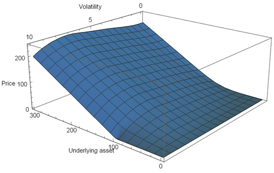
Figure 1. A numerical solution based on AFDM in Heston–Hull–White (HHW) option b.

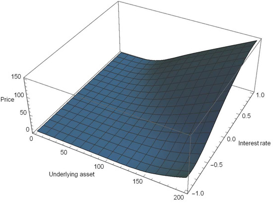
Figure 2. A numerical solution based on AFDM in HHW option b.

5. Ending Comments

In financial engineering, it is famous that the Black–Scholes PDE could not be useful in real application due to several restrictions. Several ideas to observe the market’s reality are models based upon the stochastic volatility and interest rate models. The resulted PDE problem in this way is hard to be solved theoretically due to higher involved dimensions and so numerical methods are required.

In this paper, we have proposed a new discretized numerical method based on adaptive FD methodology on non-uniform grids in order to tackle an important problem in computational finance known as HHW PDE (1). It was proved that the new procedure has conditional stability and shown to be efficient in practice.

Further discussions can be investigated to extend the results of this work for other types of options defined on HHW model such as digital (binary) options, at which the initial condition is not only non-smooth at the strike but also discontinues.

References

- Brigo, D.; Mercurio, F. Interest Rate Models-Theory and Practice: With Smile, Inflation and Credit, 2nd ed.; Springer Finance: Berlin, Germany, 2007. [Google Scholar]
- Cakici, N.; Chatterjee, S.; Chen, R.-R. Default risk and cross section of returns. J. Risk Financ. Manag. 2019, 12, 95. [Google Scholar] [CrossRef]
- Ballestra, L.V.; Cecere, L. A numerical method to estimate the parameters of the CEV model implied by American option prices: Evidence from NYSE. Chaos Solitons Fractals 2016, 88, 100–106. [Google Scholar] [CrossRef]
- Duffy, D.J. Finite Difference Methods in Financial Engineering: A Partial Differential Equation Approach; Wiley: Chichester, UK, 2006. [Google Scholar]
- Magoulès, F.; Gbikpi-Benissan, G.; Zou, Q. Asynchronous iterations of parareal algorithm for option pricing models. Mathematics 2018, 6, 45. [Google Scholar] [CrossRef]
- Fouque, J.-P.; Papanicolaou, G.; Sircar, K.R. Derivatives in Financial Markets with Stochastic Volatility; Cambridge Univ. Press: Cambridge, UK, 2000. [Google Scholar]
- Heston, S.L. A closed-form solution for options with stochastic volatility with applications to bond and currency options. Rev. Finan. Stud. 1993, 6, 327–343. [Google Scholar] [CrossRef]
- Hull, J.; White, A. Using Hull-White interest rate trees. J. Deriv. 1996, 4, 26–36. [Google Scholar] [CrossRef]
- Schöbel, R.; Zhu, J. Stochastic volatility with an Ornstein-Uhlenbeck process: An extension. Eur. Financ. Rev. 1999, 3, 23–46. [Google Scholar] [CrossRef]
- Guo, S.; Grzelak, L.A.; Oosterlee, C.W. Analysis of an affine version of the Heston-Hull-White option pricing partial differential equation. Appl. Numer. Math. 2013, 72, 143–159. [Google Scholar] [CrossRef]
- Sargolzaei, P.; Soleymani, F. A new finite difference method for numerical solution of Black-Scholes PDE. Adv. Diff. Equat. Control Process. 2010, 6, 49–55. [Google Scholar]
- Soleymani, F.; Barfeie, M. Pricing options under stochastic volatility jump model: A stable adaptive scheme. Appl. Numer. Math. 2019, 145, 69–89. [Google Scholar] [CrossRef]
- Haentjens, T.; In’t Hout, K.J. Alternating direction implicit finite difference schemes for the Heston-Hull-White partial differential equation. J. Comput. Fin. 2012, 16, 83–110. [Google Scholar] [CrossRef]
- Soleymani, F.; Akgül, A. Asset pricing for an affine jump-diffusion model using an FD method of lines on non-uniform meshes. Math. Meth. Appl. Sci. 2019, 42, 578–591. [Google Scholar] [CrossRef]
- Itkin, A.; Carr, P. Jumps without tears: A new splitting technology for Barrier options. Int. J. Numer. Anal. Model. 2011, 8, 667–704. [Google Scholar]
- Sumei, Z.; Jieqiong, Z. Efficient simulation for pricing barrier options with two-factor stochastic volatility and stochastic interest rate. Math. Prob. Eng. 2017, 2017, 3912036. [Google Scholar] [CrossRef]
- Soleymani, F.; Saray, B.N. Pricing the financial Heston-Hull-White model with arbitrary correlation factors via an adaptive FDM. Comput. Math. Appl. 2019, 77, 1107–1123. [Google Scholar] [CrossRef]
- Kwok, Y.K. Mathematical Models of Financial Derivatives, 2nd ed.; Springer: Heidelberg, Germany, 2008. [Google Scholar]
- Ballestra, L.V.; Sgarra, C. he evaluation of American options in a stochastic volatility model with jumps: An efficient finite element approach. Comput. Math. Appl. 2010, 60, 1571–1590. [Google Scholar] [CrossRef]
- Fornberg, B. A Practical Guide to Pseudospectral Methods; Cambridge University Press: Cambridge, UK, 1996. [Google Scholar]
- Soleymani, F.; Barfeie, M.; Khaksar Haghani, F. Inverse multi-quadric RBF for computing the weights of FD method: Application to American options. Commun. Nonlinear Sci. Numer. Simul. 2018, 64, 74–88. [Google Scholar] [CrossRef]
- Wellin, P.R.; Gaylord, R.J.; Kamin, S.N. An Introduction to Programming with Mathematica, 3rd ed.; Cambridge University Press: Cambridge, UK, 2005. [Google Scholar]
- Sofroniou, M.; Knapp, R. Advanced Numerical Differential Equation Solving in Mathematica, Wolfram Mathematica, Tutorial Collection; Wolfram Research, Inc.: Champaign, IL, USA, 2008. [Google Scholar]
- Luther, H.A. An explicit sixth-order Runge-Kutta formula. Math. Comput. 1967, 22, 434–436. [Google Scholar] [CrossRef]
- Mangano, S. Mathematica Cookbook; O’Reilly Media: Sevastopol, CA, USA, 2010. [Google Scholar]
© 2019 by the author. Licensee MDPI, Basel, Switzerland. This article is an open access article distributed under the terms and conditions of the Creative Commons Attribution (CC BY) license (http://creativecommons.org/licenses/by/4.0/).