Use the K-Neighborhood Subgraphs to Compute Canonical Labelings of Graphs

Abstract

This paper puts forward an innovative theory and method to calculate the canonical labelings of graphs that are distinct to $Nauty$’s. It shows the correlation between the canonical labeling of a graph and the canonical labeling of its complement graph. It regularly examines the link between computing the canonical labeling of a graph and the canonical labeling of its $open$ k-$neighborhood$ $subgraph$. It defines $diffusion$ $degree$ $sequences$ and $entire$ $diffusion$ $degree$ $sequence$. For each node of a graph G, it designs a characteristic $m\_NearestNode$ to improve the precision for calculating canonical labeling. Two theorems established here display how to compute the first nodes of $MaxQ\left(G\right)$. Another theorem presents how to determine the second nodes of $MaxQ\left(G\right)$. When computing $C_{max}\left(G\right)$, if $MaxQ\left(G\right)$ already holds the first i nodes $u_1,u_2,\cdots ,u_i$, Diffusion and Nearest Node theorems provide skill on how to pick the succeeding node of $MaxQ\left(G\right)$. Further, it also establishes two theorems to determine the $C_{max}\left(G\right)$ of disconnected graphs. Four algorithms implemented here demonstrate how to compute $MaxQ\left(G\right)$ of a graph. From the results of the software experiment, the accuracy of our algorithms is preliminarily confirmed. Our method can be employed to mine the frequent subgraph. We also conjecture that if there is a node $v\in S\left(G\right)$ meeting conditions $C_{max}(G-v)$⩽$C_{max}(G-w)$ for each $w\in S\left(G\right)\wedge w\ne v$, then $u_1=v$ for $MaxQ\left(G\right)$.

1. Introduction

This paper is the close companion to Reference [1], in which a novel theory and method are presented for calculating the canonical labelings of digraphs. The center subgraph $Cen\left(G\right)$ [2] can also be used to determine the first vertex $u_1$ added into $MaxQ\left(G\right)$ of undirected graphs.

This article concentrates on the construction of a universal system and a way of calculating the $canonical$ $labeling$ $C_{max}\left(G\right)$ of undirected graphs [3,4,5], which is also called an $optimum$ $code$ [6], a $canonical$ $code$ [7] or a canonical form [8] and is the single string corresponding one-to-one to a graph such that two graphs are isomorphic if and only if both have the accurate same canonical labelings. Currently, the calculation of the $canonical$ $labeling$ as the graph isomorphism problem is an unsolved challenge in computational complexity theory such that no polynomial-time algorithm appears for calculating the $canonical$ $labeling$ of an undirected graph. The study of canonical labeling has contributed to the studies of problems in many fields, including quantum chemistry [9], biochemistry [10,11] and so on.

Many exponential algorithms have emerged to deal with the problem. However, different researchers like to define different canonical labeling. Given a graph of n vertices, Kuramochi and Karypis build the canonical labeling by concatenating the columns of the upper-triangular part of its adjacency matrix [12,13]. Huan et al. concatenate the lower triangular elements (including the diagonal elements) of its adjacency matrix to create its canonical labeling [14]. Kashani et al. determine the canonical labeling by concatenating the rows of its adjacency matrix to form an $n^2$ binary number [15,16]. Each of these canonical labelings correspondings one-to-one to a lexicographically smallest graph whose adjacency matrix is seen as a linear string, which is lexicographically smallest. Nevertheless, the computation of the lexicographically least graph is $NP$-hard [8,17].

Throughout the paper, the $canonical$ $labeling$ $C_{max}\left(G\right)$ of a graph G is the lexicographically largest string constructed by concatenating the rows of the upper triangular portion of the adjacency matrix associated with G (see Definition 5). The computational complexity that determines the $canonical$ $labeling$ $C_{max}\left(G\right)$ of G is also $NP$-hard.

Babai and Luks used a general group-theoretic method to calculate canonical labeling [8]. Nevertheless, combinatorial approaches have operated well in numerous particular situations. For stochastic graphs, Babai et al. generate canonical labeling with high possibility [8,18]. Arvind et al. introduce two similar logspace algorithms for partial 2- and 3-Trees [17,19].

Currently, $Nauty$ is the most prevalent and pragmatic means for determining the automorphism group and the $canonical$ $labelings$ of graphs [3,20,21,22]. It appears to have shifted the industry norm for determining the $canonical$ $labeling$ also the automorphism group. For calculating the $canonical$ $labeling$ and automorphism group, $Nauty$ and Yan and Han [23] use the depth-first search to traverse the latent intermediary vertices in the search tree. The vertices of the search tree produced by $Nauty$ are equitable ordered partitions of vertices in G. $Nauty$ iteratively refines partitioning vertices until places the vertices that have the exact equivalent features into an automorphism orbit. As the partition refinement becomes finer and finer, it automatically makes the $canonical$ $labeling$. Nonetheless, $Nauty$ also needs exponential time to calculate the canonical labeling for a given Miyazaki graph [24]. Tener and Deo earned advances for processing the problem [25].

Besides $Nauty$, $Traces$ [4], $Bliss$ [5,26] and Conauto [27] are all state-of-the-art tools for graphs isomorphism testing. Based on the individualization of nodes, backtracking and partition refinement, $Bliss$ [5,26] is powerful canonical labeling means for dealing with large and sparse graphs. Katebi et al. combine $Saucy$ with $Bliss$ and show that it is faster for computing the automorphism group of a graph with $Saucy$ and then calculating its canonical labeling with $Bliss$ than for alone calculating its canonical labeling with $Bliss$ [28]. To fix the vulnerability of $Nauty$, $Traces$ uses the policy of breadth-first search to decide the automorphism group and the canonical labeling [4]. $Conauto$ also utilizes the fundamental individualization/refinement method and is quite quick for random graphs and several classes of hard graphs.

For the advancement of performance, current algorithms usually employ backtracking and orbit partitioning way to circumvent frequently visiting the same nodes and contrive to decrease the accessed nodes in the search tree. For the canonical labeling issue, McKay et al. present a full examination of the problem [22,23].

$Nauty$ governed the area for several decades. Therefore, in-depth research for canonical labeling has been limited to the theoretical skeleton of $Nauty$. This implies that people are only like to support the study trajectory of $nauty$ to extend and build further research.

Since there are several different definitions of canonical labeling, there is no uniform standard such that each researcher works on oneself standard. Besides the lack of a unified standard, the research on the connection between the distinct canonical labeling is also quite lacking. It is a hard task that one wants to confirm the accuracy of canonical labeling achieved by executing an algorithm. Up to now, the criterion by which one can decide which definition is better does not appear.

In this paper, the definition of $canonical$ $labeling$ is completely distinct that of $nauty$. Unless by chance, the canonical labeling produced by $Nauty$ will be not a $canonical$ $labeling$ according to the definition presented by the paper. It is sometimes difficult to confirm the accuracy of the canonical labeling achieved by executing $Nauty$ according to the criterion of $Nauty$. Since the insides of many graphs contain a large number of automorphisms, the calculation of canonical labeling becomes extremely arduous in certain situations.

A graph invariant $I\left(G\right)$ is called complete if the equality of the invariants $I\left(G\right)$ and $I\left(H\right)$ implies the isomorphism of the graphs G and H. However, even polynomial-valued invariants such as the chromatic polynomial are not usually complete. A path graph is a graph consisting of exactly its maximal path. For example, the path graph with 4 vertices and the claw graph $K_{1,3}$ both have the same chromatic polynomial.

Many algorithms also use the identical definition of $canonical$ $labeling$ as adopted in the paper. However, their main goal is not to consider how to calculate $canonical$ $labeling$ but for other purposes such as mining the frequent subgraphs. Therefore, these algorithms can only run for some limited graph classes. Until now, based on current knowledge and Definition 5 present in this paper, a universal algorithm for calculating the $canonical$ $labelings$ of graphs does not appear.

Jianqiang Hao et al. also provide Propositions 5–6, Lemmas 1–3 and Theorems 10–13 in Reference [2] by which one can compute the proper vertices added into $MaxQ\left(G\right)$. However, they do not give any proof. In this article, we prove Theorems 3–6 that are one-to-one corresponding to Theorems 10–13 in Reference [2]. We also present the reasons for Lemmas 8–9, which are one-to-one corresponding to Lemmas 2–3 in Reference [2].

In the rest of this paper, Section 2 presents some fundamental vocabulary and preparatory knowledge. Section 3 represents the results followed by some analysis. Section 4 gives our algorithms for calculating the $canonical$ $labeling$. Section 5 demonstrates the implementation of our algorithms and evaluates our way through many examples. Finally, Section 6 remarks on our conclusions and future work.

2. Preliminaries

This paper only handles limited undirected graphs with neither loops nor multiple edges. A graph consists of a set of nodes and a collection of edges. For a graph $G=\left(V\right(G)$, $E\left(G\right))$, assume that $V\left(G\right)$ and $E\left(G\right)$ represent the set of vertices of G and the collection of edges of G. Any an edge $(u,v)\in E\left(G\right)$ joins two vertices $u\in G$ and $v\in G$. For this article to be self-contained, the relevant concepts and definitions are given below.

Definition 1.

Suppose $G=\left(V\right(G)$, $E\left(G\right))$ is an undirected graph of n vertices. A vertex-induced subdigraph on $V_1\subseteq V\left(G\right)$ of G is a subgraph with the vertices set $V_1$ together with any side whose endpoints are both in $V_1$, expressed by $G\left[V_1\right]$.

Definition 2.

Given two undirected graphs $G=\left(V\right(G)$, $E\left(G\right))$ and $H=\left(V\right(H)$, $E\left(H\right))$ of n vertices. If there is a bijection $f:V\left(G\right)\to V\left(H\right)$ such that $\forall (u,v)\in E\left(G\right)$ if and only if $\left(f\right(u),f(v\left)\right)\in E\left(H\right)$. We call f an isomorphic projection of $G\to H$. Furthermore, we state that the graph G and H are isomorphic, signified by $G\cong H$. An isomorphic map f of G onto itself is declared to be an automorphism of G.

Let $X=(x_1,x_2,\cdots$, $x_i,\cdots x_m)$ in $R^m$ and $Y=(y_1,y_2,\cdots$, $y_j$, ⋯$y_n)$ in $R^n$ be two vectors, the issue emerges as to how to determine which one is larger. When comparing two vectors, the following rules must be satisfied.

Definition 3.

Given two vectors $X=(x_0,x_1,\cdots$, $x_i,\cdots x_m)$ and $Y=(y_0,y_1,\cdots ,y_i,\cdots y_n)$ in N (the collection of natural numbers) satisfying $m\ge 0$ and $n\ge 0$. Then, the lexicographic order of the two vectors is defined as follows:

1. 

$X=Y$, if $m=n$ and $x_i=y_i$ for all $0\le i\le m$.

2. 

$X<Y$ if and only if either of the following is true.

(a) 

$\exists k,0\le k\le min(m,n),x_i=y_i$ for $i<k$, $x_k<y_k$.

(b) 

$x_i=y_i$ for $0\le i\le m$ and $m<n$.

Definition 4.

Given two vectors $Z_1=(X_0,X_1,\cdots$, $X_i,\cdots X_m)$ and $Z_2=(Y_0,Y_1,\cdots ,Y_j,\cdots Y_n)$ satisfying $m\ge 0$ and $n\ge 0$, where each $X_i$, $Y_j,i=0,1,\cdots ,m,j=0,1,\cdots ,n$ denotes a vector in N (the collection of natural numbers). Then, the lexicographic order of the two vectors is defined as follows:

1. 

$Z_1=Z_2$, if $m=n$ and $X_i=Y_i$ for all $0\le i\le m$.

2. 

$Z_1<Z_2$ if and only if either of the following is true.

(a) 

$\exists k,0\le k\le min(m,n),X_i=Y_i$ for $i<k$, $x_k<y_k$.

(b) 

$X_i=Y_i$ for $0\le i\le m$ and $m<n$.

Definition 5.

Suppose $G=\left(V\right(G)$, $E\left(G\right))$ is an undirected graph of n vertices with adjacency matrix $A\left(G\right)$ $={\left(a_{i,j}\right)}_{n\times n}$. To concatenate the rows of the upper triangular part of $A\left(G\right)$ in the following order $a_{1,2}$, $a_{1,3}$, ⋯, $a_{1,n}$, $a_{2,3}$, $a_{2,4}$, ⋯, $a_{2,n}$, ⋯, $a_{i,i+1}$, $a_{i,i+2}$, ⋯, $a_{i,n}$, ⋯, $a_{n-1,n}$ makes a corresponding binary number $a_{1,2}{a}_{1,3}\cdots a_{1,n}$ $a_{2,3}{a}_{2,4}$ $\cdots a_{2,n}\cdots a_{i,i+1}{a}_{i,i+2}\cdots a_{i,n}$ $\cdots a_{n-1,n}$, which is a$labeling$of G, signified by$C\left(G\right)$ (see (1)).

$$\begin{array}{ccc}\hfill A\left(G\right)& =& \left(\begin{array}{cccccccc}0& \to a_{1,2}& \to a_{1,3}& \cdots & \cdots & \cdots & \cdots & \to a_{1,n}\hfill \\ a_{1,2}& 0& \to a_{2,3}& \cdots & \cdots & \cdots & \cdots & \to a_{2,n}\hfill \\ ⋮& \cdots & \ddots & \cdots & \cdots & \cdots & \cdots & \downarrow ⋮\hfill \\ ⋮& \cdots & \cdots & \ddots & \cdots & \cdots & \cdots & \downarrow ⋮\hfill \\ a_{1,i}& a_{2,i}& \cdots & a_{i,i-1}& 0& \to a_{i,i+1}& \cdots & \to a_{i,n}\hfill \\ ⋮& \cdots & \cdots & \cdots & \cdots & \ddots & \cdots & \downarrow ⋮\hfill \\ ⋮& \cdots & \cdots & \cdots & \cdots & \cdots & \ddots & \to a_{n-1,n}\hfill \\ a_{1,n}& a_{2,n}& a_{3,n}& \cdots & \cdots & \cdots & a_{n-1,n}& 0\hfill \end{array}\right)\hfill \end{array}$$

(1)

The first row of the upper triangular portion of $A\left(G\right)$ is the $labeling$ $slice$ 1 of $C\left(G\right)$, signified by $C^1\left(G\right)$. Likewise, the second row of the upper triangular portion is the $labeling$ $slice$ 2 of $C\left(G\right)$, signified by $C^2\left(G\right)$. ⋯. The $(n-1)$th row of the upper triangular portion is the $labeling$ $slice$ $n-1$ of $C\left(G\right)$, signified by $C^{n-1}\left(G\right)$. It is true that $C\left(G\right)=C^1\left(G\right)C^2\left(G\right)\cdots C^{n-1}\left(G\right)$.

A permutation $\pi$ of the nodes of G is an order of the n nodes without repeating. The number of shifts of the nodes of G is $n!$. Further, each distinct permutation $\pi$ of the n nodes of $V\left(G\right)$ determines a single adjacency matrix. Therefore, given a permutation $\pi$, one can get a $labeling$ $C\left(G\right)$ corresponding to $\pi$ by Definition 5. The collection of all $labeling$ of G is represented by $L\left(G\right)$.

For every $C_1\left(G\right)$, $C_2\left(G\right)\in L\left(G\right)$, Suppose that $C_1\left(G\right)=i_1{i}_2\cdots i_m$, $C_2\left(G\right)=j_1{j}_2\cdots j_n$ with $i_1,i_2,\cdots ,i_m$, $j_1,j_2,\cdots ,j_n=0$ or 1. Given $X=(i_1,i_2,\cdots ,i_m)$ and $Y=(j_1,j_2,\cdots ,\cdots j_n)$. By Definition 3, if $X>Y$, then we set $C_1\left(G\right)>C_2\left(G\right)$. Otherwise, if $X<Y$, then we set $C_1\left(G\right)<C_2\left(G\right)$. Otherwise, if $X=Y$, then we set $C_1\left(G\right)=C_2\left(G\right)$.

Definitely, $\left(L\right(G)$, $\le )$ is a well-ordered set, where ≤ signifies the less-than-or-equal-to binary relationship on the collection $L\left(G\right)$ stated as above. By the well-ordering theorem, it follows that $L\left(G\right)$ has a minimum and maximum element, signifies by $C_{min}\left(G\right)$ and $C_{max}\left(G\right)$ and called $minimum$ $canonical$ $labeling$ of G and $maximum$ $canonical$ $labeling$ of G respectively. We also call $maximum$ $canonical$ $labeling$$canonical$ $labeling$ of G.

The two shifts of the n nodes of G associated with $C_{min}\left(G\right)$ and $C_{max}\left(G\right)$ are the $minimum$ $and$ $maximum$ $node$ $sequence$, signifies by $MinQ\left(G\right)$ and $MaxQ\left(G\right)$. Furthermore, the two adjacency matrices of G associated with $C_{min}\left(G\right)$ and $C_{max}\left(G\right)$ are the $minimum$ $and$ $maximum$ $canonical$ $labeling$ $matrix$, signifies by $A_{min}\left(G\right)$ and $A_{max}\left(G\right)$.

$C^1\left(G\right),C^2\left(G\right),\cdots ,C^{n-1}\left(G\right)$ corresponding to $A_{min}\left(G\right)$ are $minimum$ $canonical$ $labeling$ $slice$ $1,2,\cdots ,n-1$ of canonical labeling $C\left(G\right)$, signified by $C_{min}^1\left(G\right)$, $C_{min}^2\left(G\right)$, ⋯, $C_{min}^{n-1}\left(G\right)$, respectively. Conversely, $C^1\left(G\right)$, $C^2\left(G\right)$, ⋯, $C^{n-1}\left(G\right)$ corresponding to $A_{max}\left(G\right)$ are $maximum$ $canonical$ $labeling$ $slice$ $1,2,\cdots ,n-1$ of canonical labeling $C\left(G\right)$, signified by $C_{max}^1\left(G\right)$, $C_{max}^2\left(G\right)$, ⋯, $C_{max}^{n-1}\left(G\right)$, respectively.

Based on the above definitions, the following equations are established.

$$\begin{array}{ccc}\hfill C_{min}\left(G\right)& =& C_{min}^1\left(G\right)C_{min}^2\left(G\right)\cdots C_{min}^{n-1}\left(G\right)\hfill \end{array}$$

(2)

$$\begin{array}{ccc}\hfill C_{max}\left(G\right)& =& C_{max}^1\left(G\right)C_{max}^2\left(G\right)\cdots C_{max}^{n-1}\left(G\right)\hfill \end{array}$$

(3)

Theorem 1.

Given two undirected graphs $G=\left(V\right(G)$, $E\left(G\right))$ and $H=\left(V\right(H)$, $E\left(H\right))$ of n vertices with adjacency matrices $A\left(G\right)$ and $A\left(H\right)$ respectively. Then $G\cong H$ if and only if $C_{min}\left(G\right)$=$C_{min}\left(H\right)$ or $C_{max}\left(G\right)$=$C_{max}\left(H\right)$.

Lemma 1.

Suppose $G=\left(V\right(G)$, $E\left(G\right))$ is an undirected graph of n vertices whose complement graph is $\overline{G}=(V\left(\overline{G}\right)$, $E\left(\overline{G}\right))$. Then $C\left(G\right)=\overline{C\left(\overline{G}\right)}$ and $C\left(\overline{G}\right)=\overline{C\left(G\right)}$ hold.

Proof. 

The adjacency matrices of G and $\overline{G}$ meet the following condition.

$$A\left(G\right)+A\left(\overline{G}\right)=J=\left(\begin{array}{ccccc}0& 1& \cdots & \cdots & 1\\ 1& 0& 1& \cdots & ⋮\\ ⋮& 1& 0& 1& ⋮\\ ⋮& ⋮& 1& \ddots & 1\\ 1& \cdots & \cdots & 1& 0\end{array}\right).$$

where J is an $n\times n$ matrix of zeros and ones whose main diagonal entries are 0 and all other entries are 1. By the complement graph $\overline{G}$ and $A\left(G\right)=J-A\left(\overline{G}\right)$, it can be seen that $C\left(G\right)=\overline{C\left(\overline{G}\right)}$. Furthermore, by $A\left(\overline{G}\right)=J-A\left(G\right)$, it follows that $C\left(\overline{G}\right)=\overline{C\left(G\right)}$ for the complement graph $\overline{G}$ of G. □

Theorem 2.

Suppose $G=\left(V\right(G)$, $E\left(G\right))$ is an undirected graph of n vertices whose complement graph is $\overline{G}=(V\left(\overline{G}\right)$, $E\left(\overline{G}\right))$. It follows that

$$\begin{array}{ccc}\hfill C_{min}\left(G\right)& =& \overline{C_{max}\left(\overline{G}\right)}\hfill \end{array}$$

(4)

$$\begin{array}{ccc}\hfill C_{max}\left(G\right)& =& \overline{C_{min}\left(\overline{G}\right)}\hfill \end{array}$$

(5)

$$\begin{array}{ccc}\hfill C_{min}\left(\overline{G}\right)& =& \overline{C_{max}\left(G\right)}\hfill \end{array}$$

(6)

$$\begin{array}{ccc}\hfill C_{max}\left(\overline{G}\right)& =& \overline{C_{min}\left(G\right)}\hfill \end{array}$$

(7)

Proof. 

By Lemma 1, it holds that $C\left(G\right)=\overline{C\left(\overline{G}\right)}$. Definitely, the k-bit of $C\left(\overline{G}\right)$ is 0 if and only if the k-bit of $C\left(G\right)$ is 1. Therefore, one can make the $canonical$ $labeling$ $C_{max}\left(G\right)$ of G by executing a complement operation on $C_{min}\left(\overline{G}\right)$. Likewise, by Lemma 1, the identity $C\left(\overline{G}\right)=\overline{C\left(G\right)}$ holds. Definitely, the k-bit of $C\left(G\right)$ is 0 if and only if the k-bit of $C\left(\overline{G}\right)$ is 1. Hence, one can make the $canonical$ $labeling$ $C_{max}\left(\overline{G}\right)$ of $\overline{G}$ by executing a complement operation on $C_{min}\left(G\right)$.

Since $C\left(K_n\right)$ is a constant binary number, one must maximize $C\left(\overline{G}\right)$ to minimize $C\left(G\right)$. On the opposite, one must minimize $C\left(\overline{G}\right)$ to maximize $C\left(G\right)$. Likewise, one must maximize $C\left(G\right)$ to minimize $C\left(\overline{G}\right)$. Contrariwise, one must minimize $C\left(G\right)$ to maximize $C\left(\overline{G}\right)$. From the above examination, the following results hold.

$$\begin{array}{cccc}\hfill C_{min}\left(G\right)& =\overline{C_{max}\left(\overline{G}\right)}.\hfill & \hfill C_{max}\left(G\right)& =\overline{C_{min}\left(\overline{G}\right)}.\hfill \\ \hfill C_{min}\left(\overline{G}\right)& =\overline{C_{max}\left(G\right)}.\hfill & \hfill C_{max}\left(\overline{G}\right)& =\overline{C_{min}\left(G\right)}.\hfill \end{array}$$

 □

By Theorem 2, it can be seen that if one has computed the $C_{max}\left(\overline{G}\right)$, one can simply make $C_{min}\left(G\right)$. Moreover, the computation means of $C_{max}\left(\overline{G}\right)$ and $C_{max}\left(G\right)$ are precisely the same.

Theorem 2 shows the mutual relations between $C_{max}\left(G\right)$ and $C_{min}\left(G\right)$. Because of the existence of the relations, the paper only concentrates on the construction of effective ways to determine $C_{max}\left(G\right)$. The $TopMost$ $graph$ of G is a graph whose $labeling$ $C\left(G\right)$ is lexicographically largest.

We signify by $d_G\left(u\right)$ the degree of a node u in G, by $d\left(G\right)=(d_G\left(u_1\right),d_G\left(u_2\right),\cdots$, $d_G\left(u_n\right))$ the $degree$ $sequence$ of G, by $d_G\left(V_1\right)=(d_G\left(v_1\right),d_G\left(v_2\right),\cdots ,d_G\left(v_m\right))$ the degree series of a subset $V_1\subseteq V\left(G\right)$ with $v_i\in V_1$, $i=1,2,\cdots ,m$ and by $d_G\left(H\right)=(d_H\left(w_1\right),d_H\left(w_2\right)$, $\cdots ,d_H\left(w_s\right))$ the $degree$ $sequence$ of a subgraph $H\subseteq G$ with $w_j\in V\left(H\right)$, $j=1,2,\cdots ,t$ and drop the symbol G when no vagueness can occur. We signify by $\delta \left(G\right)$ the minimum degree and by $\Delta \left(G\right)$ the maximum degree of all vertices of a graph G. Throughout this article, suppose $S\left(G\right)=\left\{u\right|u\in V\left(G\right)\wedge$ $d\left(u\right)=\Delta \left(G\right)\}$. In the following text, when simultaneously involving two graphs, we always assume that their degree sequences are the same except specified.

For each $u\in V\left(G\right)$, the quantity of vertices with degree $d_G\left(u\right)$ is the $degree$ $multiplicity$ of u, signified by $d{m}_G\left(u\right)$. Unless otherwise specified, throughout this article, the degree sequence is decreasing. The distance $d(u,v)$ between any two nodes u and v is the number of edges on the shortest path from u to v.

For every $u\in V\left(G\right)$, an edge connecting two adjacent vertices of u is a $chord$ $edge$ of u and an edge connecting u and its an adjacent vertex is an $incident$ $edge$ of u. Given a set S of vertices in G, let $CE$$\left(S\right)$ signify the $set$ $of$ $chord$ $edges$ of all nodes in S and $IE$$\left(S\right)$ signify the $set$ $of$ $incident$ $edges$ of all vertices in S. Such as in the graph G shown in Figure 1, the edge $(3,8)$ is a $chord$ $edge$ of the vertex 7 and each of the edges $(3,7)$, $(7,8)$ and $(10,7)$ are its $incident$ $edges$. $CE\left(\right\{7\left\}\right)=\left\{\right(3,8\left)\right\}$ and $IE\left(\right\{7\left\}\right)=\left\{\right(3,7),(7,8),(10,7\left)\right\}$.

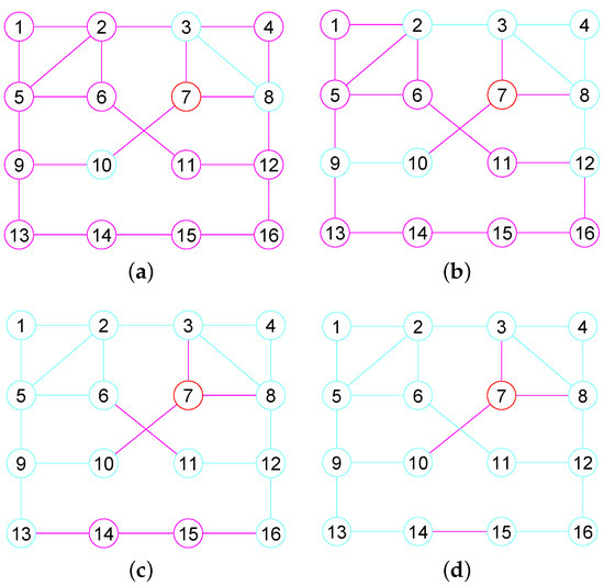
Figure 1. The 1, 2, 3, 4-neighborhood subgraph of vertex 7 in a graph G. (a) The 1-neighbor subgraph; (b) The 2-neighbor subgraph; (c) The 3-neighbor subgraph; (d) The 4-neighbor subgraph.

Definition 6.

Suppose $G=\left(V\right(G)$, $E\left(G\right))$ is an undirected graph of n vertices. The open neighborhood subgraph of a node u in G is a subgraph of G, signified by $N\left(u\right)=\left(V\right(N\left(u\right))$, $E\left(N\right(u\left)\right))$ where $V\left(N\right(u\left)\right)$ is the set of all nodes adjacent to u ($u\notin V\left(N\right(u\left)\right)$) and $E\left(N\right(u\left)\right)$ is the collection of all edges, each of which connects two vertices of $V\left(N\right(u\left)\right)$.

The $open$ k-$neighborhood$ $subgraph$ of u with $k\ge 2$ is a subgraph, signified by $N_k\left(u\right)=$ $\left(V\right(N_k$ $\left(u\right))$, $E(N_k$ $\left(u\right)\left)\right)$ with $V\left(N_k\left(u\right)\right)=\{v\mid d(u,v)\le k\wedge v\ne u\wedge v\in V\left(G\right)\}$, $E\left(N_k\left(u\right)\right)=\left\{\right(v,$ $w)$ $\mid v,w\in V\left(N_k\left(u\right)\right),(v,w)\in CE\left(V\left(N_{k-1}\left(u\right)\right)\right)\vee IE\left(V\left(N_{k-1}\left(u\right)\right)\right)\}$.

Definition 7.

Suppose $G=\left(V\right(G)$, $E\left(G\right))$ is an undirected graph of n vertices. The open neighborhood subgraph of a vertices set $Q\subseteq V\left(G\right)$ is a subgraph of G, signified by $N\left(Q\right)=$ $\left(V\right(N\left(Q\right)),E(N\left(Q\right)\left)\right)$ where $V\left(N\right(Q\left)\right)$ is the set of all nodes each of which is adjacent to at least one node in Q with $Q\cap V\left(N\right(Q\left)\right)=\varnothing$ and $E\left(N\right(Q\left)\right)$ is the collection of all edges each of which joins two vertices of $V\left(N\right(Q\left)\right)$.

The $open$ k-$neighborhood$ $subgraph$ of Q with $k\ge 2$ is a subgraph, signified by $N_k\left(Q\right)=$ $\left(V\right(N_k$ $\left(Q\right)),E(N_k$ $\left(Q\right)\left)\right)$ with $V\left(N_k\left(Q\right)\right)=\{v\mid v\notin Q\wedge v\in V\left(G\right)\wedge \exists u\in Q\wedge d(v,u)\le k\}$, $E(N_k$ $\left(Q\right))$ $=\{(v,w)\mid v,w\in V\left(N_k\left(Q\right)\right),(v,w)\in CE\left(V\left(N_{k-1}\left(Q\right)\right)\right)\vee IE(V$ $\left(N_{k-1}\left(Q\right)\right)\left)\right\}$.

Remark 1.

For some graphs, there may be some edges whose two end vertices lie in $V\left(N_k\left(u\right)\right)$ but do not belong to $N_k\left(u\right)$ by Definition 6. For example, consider the graph G given in Figure 1. Although the vertex 6 and 11 belong to $V\left(N_3\left(7\right)\right)$, $(6,11)\notin E\left(N_3\left(7\right)\right)$. In addition, the vertex 14 and 15 belong to $V\left(N_4\left(7\right)\right)$. However, $(14,15)\notin E\left(N_4\left(7\right)\right)$.

Definition 8.

Suppose $G=\left(V\right(G)$, $E\left(G\right))$ is an undirected graph of n vertices. For each $u\in V\left(G\right)$, the open kth neighborhood subgraph of u with $k\ge 0$ is a subgraph, signified by $T_k\left(u\right)=(V\left(T_k\left(u\right)\right),E\left(T_k\left(u\right)\right))$ with $V\left(T_k\left(u\right)\right)$ $=\{v\mid d(u,v)=k\wedge v\ne u\wedge v\in V(G\left)\right\}$, $E\left(T_k\left(u\right)\right)$ $=\{(v,w)\mid v,w\in V\left(T_k\left(u\right)\right)\wedge (v,w)$ $\in CE\left(V\left(T_k\left(u\right)\right)\right)\}$. For $k=0$, let $V\left(T_0\left(u\right)\right)=\left\{u\right\}$ and $E\left(T_0\left(u\right)\right)=\varnothing$.

Definition 9.

Suppose $G=\left(V\right(G)$, $E\left(G\right))$ is an undirected graph of n vertices. Assume that $H\subseteq G$ and $u\in V\left(H\right)$. We signify by $N_H^k\left(u\right)$ the$open$k-$neighborhood$$subgraph$of u in H and by$T_H^k\left(u\right)$the $open$$kth$ $neighborhood$$subgraph$ of u in H. For $k=1$, we drop the superscript 1 for clarity and write $N_H\left(u\right)=N_H^1\left(u\right)$ and $T_H\left(u\right)=T_H^1\left(u\right)$, instead.

Definition 10.

Suppose $G=\left(V\right(G)$, $E\left(G\right))$ is an undirected connected graph of n vertices. For each $u\in V\left(G\right)$, there is a positive integer k meeting conditions $N_{k-1}\left(u\right)\subset G-u$ and $N_k\left(u\right)=G-u$. The value of k is defined as the$diffusion$$radius$ of u, signified by ${\rho }_G\left(u\right)$ and we drop the symbol G when no vagueness can occur.

By Definition 10, it is explicit that $N_{\rho \left(u\right)}\left(u\right)=G-u$ for each u in G. For notational convenience, we sometimes use $G-u$ as a shorthand for $N_{\rho \left(u\right)}\left(u\right)$.

Here, we discuss the connection between the $open$ k-$neighborhood$ $subgraph$ $N_k\left(u\right)$ and $d\left(u\right)$ with $u\in V\left(N_k\left(u\right)\right)$ (see Figure 2). We present some basic properties of the $open$ k-$neighborhood$ $subgraph$ $N_k\left(u\right)$ by the following Lemma 2.

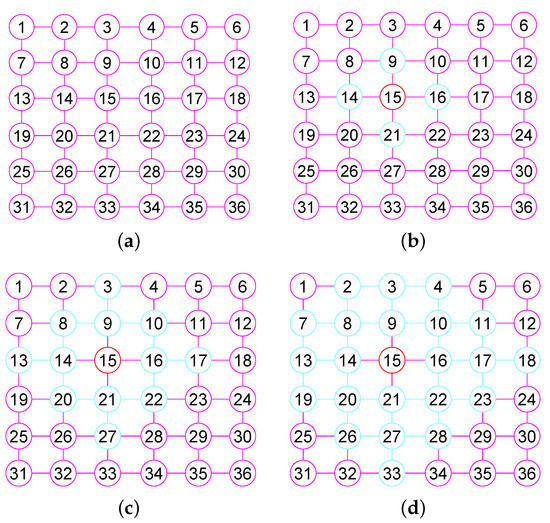
Figure 2. The 1, 2, 3-neighborhood subgraph of vertex 15 in the $6\times 6$ grid graph $G_{6,6}$. (a) The $6\times 6$ grid graph $G_{6,6}$; (b) The 1-neighbor subgraph of 15; (c) The 2-neighbor subgraph of 15; (d) The 3-neighbor subgraph of 15.

Lemma 2.

Let $N_1\left(u\right)$, $N_2\left(u\right)$, ⋯, $N_k\left(u\right)$, ⋯, $N_{\rho \left(u\right)}\left(u\right)$ be the $1,2,\cdots ,k,\cdots ,\rho \left(u\right)$-neighborhood subgraph of a vertex u in a graph G. If there exists a node $v\in V\left(N_1\left(u\right)\right)$, then

$$\begin{array}{ccc}\hfill d_{N_2\left(u\right)}\left(v\right)=d_{N_3\left(u\right)}\left(v\right)& =& \cdots =d_{N_k\left(u\right)}\left(v\right)=\cdots =d_{N_{\rho \left(u\right)}\left(u\right)}\left(v\right)=d_G\left(v\right)-1.\hfill \end{array}$$

(8)

Likewise, if there exists a node $v\notin V\left(N_k\left(u\right)\right)\wedge v\in V\left(N_{k+1}\left(u\right)\right)$ with $k\ge 1$, then

$$\begin{array}{ccc}\hfill d_{N_{k+2}\left(u\right)}\left(v\right)=d_{N_{k+3}\left(u\right)}\left(v\right)& =& \cdots =d_{N_{\rho \left(u\right)}\left(u\right)}\left(v\right)=d_G\left(v\right).\hfill \end{array}$$

(9)

Proof. 

(8) and (9) follow directly from Definition 10 (see Figure 2). □

By Lemma 2, it is clear that for every $v\in V\left(N_{k+1}\left(u\right)\right)$, satisfies $v\in V(N_k$ $\left(u\right))$ or $v\notin V(N_k$ $\left(u\right))$. According to whether v belongs to $V\left(N_k\left(u\right)\right)$ or not, $V\left(N_{k+1}\left(u\right)\right)$ can be partitioned into two disjoint sets $V_{k+1}^1\left(u\right)=\{v\mid v\in V\left(N_k\left(u\right)\right)\wedge v\in V\left(N_{k+1}\left(u\right)\right)\}$ and $V_{k+1}^2\left(u\right)=\{w\mid w\notin$ $V(N_k$ $\left(u\right))$ $\wedge w\in V\left(N_{k+1}\left(u\right)\right)\}$. Observe that $V_{k+1}^1\left(u\right)=V\left(N_k\left(u\right)\right)$ and $V_{k+1}^2\left(u\right)$ $=V\left(N\left(V_k^2\left(u\right)\right)\right)$ hold by Definitions 6 and 7 (see Figure 1). Therefore $V\left(N_{k+1}\left(u\right)\right)=V_{k+1}^1\left(u\right)\cup V_{k+1}^2\left(u\right)=V\left(N_k\left(u\right)\right)$ $\cup V(N$ $(V_k^2$ $\left(u\right)\left)\right)$. $V_{k+1}^1\left(u\right)$ and $V_{k+1}^2\left(u\right)$ are the $degree$ $stable$ $vertices$ $set$ and $degree$ $unstable$ $vertices$ $set$ of $N_{k+1}\left(u\right)$ referred to as the $stable$ $vertices$ $set$ and $unstable$ $vertices$ $set$. Correspondingly, a vertex $v\in V_{k+1}^1\left(u\right)$ is a $degree$ $stable$ $vertex$ referred to as a $stable$ $vertex$ and a vertex $w\in V_{k+1}^2\left(u\right)$ is a $degree$ $unstable$ $vertex$ referred to as an $unstable$ $vertex$.

Further note that $E\left(N_{k+1}\left(u\right)\right)=E\left(N_k\left(u\right)\right)\cup E_{k+1}$ with $E_{k+1}=CE\left(N\left(V_k^2\left(u\right)\right)\right)\cup IE$ $\left(N\right(V_k^2$ $\left(u\right)\left)\right)$. Therefore, $E\left(N_{k+1}\left(u\right)\right)=E\left(N_k\left(u\right)\right)\cup CE\left(N\left(V_k^2\left(u\right)\right)\right)\cup IE\left(N\left(V_k^2\left(u\right)\right)\right)$. The following Lemma 3 sums up the above discussion.

Lemma 3.

Suppose $N_{k+1}\left(u\right)=(V\left(N_{k+1}\left(u\right)\right),E\left(N_{k+1}\left(u\right)\right))$ is the$open$$(k+1)$-$neighborhood$$subgraph$ of vertex u in a graph G. Then there exist two disjoint sets, the $stable$ $vertices$ $set$ $V_{k+1}^1\left(u\right)$ and the $unstable$ $vertices$ $set$ $V_{k+1}^2\left(u\right)$, meeting conditions

$$\begin{array}{ccc}\hfill V\left(N_{k+1}\left(u\right)\right)& =& V_{k+1}^1\left(u\right)\cup V_{k+1}^2\left(u\right)=V\left(N_k\left(u\right)\right)\cup V\left(N\left(V_k^2\left(u\right)\right)\right),\hfill \end{array}$$

(10)

with $V_{k+1}^1\left(u\right)=V\left(N_k\left(u\right)\right)$, $V_{k+1}^2\left(u\right)=V\left(N\left(V_k^2\left(u\right)\right)\right)$. Further, it follows that

$$\begin{array}{ccc}\hfill E\left(N_{k+1}\left(u\right)\right)& =& E\left(N_k\left(u\right)\right)\cup CE\left(N\left(V_k^2\left(u\right)\right)\right)\cup IE\left(N\left(V_k^2\left(u\right)\right)\right).\hfill \end{array}$$

(11)

Let $V\left(N_0\left(u\right)\right)=\varnothing$ and $V_0^2\left(u\right)=u$, then $V_1^1\left(u\right)=\varnothing$ and $V_1^2\left(u\right)=V\left(N_1\left(u\right)\right)$ hold for the neighborhood subgraph.

For the $\rho \left(u\right)$-neighborhood subgraph, $V_{\rho \left(u\right)+1}^1\left(u\right)=V(N_{\rho \left(u\right)+1}$ $\left(u\right))=V\left(N_{\rho }\left(u\right)\right)$ holds with $V_{\rho \left(u\right)+1}^2\left(u\right)=\varnothing$.

By Lemma 3, it can be seen that the calculation of the $open$ $(k+1)$-$neighborhood$ $subgraph$ can be simplified by means of the $open$ k-$neighborhood$ $subgraph$ for every node v in G.

Definition 11.

Assume that $G=\left(V\right(G)$, $E\left(G\right))$ is an undirected graph and u is a vertex in G whose $open$ k-$neighborhood$ $subgraph$ is $N_k\left(u\right)$ with $k=1,2,\cdots$. A vertex in $N\left(u\right)$ is a$one$$diffusion$$radius$$node$ of u. For $k>1$, a node v in $N_k\left(u\right)$ meeting condition $v\notin N_{k-1}\left(u\right)$ is a  k$diffusion$$radius$$node$ of u.

Each vertex v in G is attached a property $m\_NearestNode$ whose function is explained in Section 3.1.2.

Definition 12.

Assume that $G=\left(V\right(G)$, $E\left(G\right))$ is an undirected graph and u is a node in G whose $open$ k-$neighborhood$ $subgraph$ is $N_k\left(u\right)$ with $k=1,2,\cdots$. Suppose H is a connected component of $N_k\left(u\right)$ with $k\ge 1$. Suppose that $V_m\subseteq V\left(H\right)$ with $m=0,1,2,\cdots ,t$, where $V_0$ is in ascending order of attribute $m\_NearestNode$ with

$v->m\_NearestNode$$\ge 1$ for every $v\in V_0$ and $V_1,V_2$, $\cdots ,V_t$ contain the $1,2,\cdots ,k$ $diffusion$ $radius$ $nodes$ of u respectively, meeting conditions $V_0\cup V_1\cup \cdots \cup V_t=V\left(H\right)$ and $V_i\cap V_j=\varnothing$ for $i\ne j,i,j=0,1,\cdots ,t$.

Let $d_{\sigma }\left(H\right)=(d_{N_k\left(u\right)}\left(V_0\right)$, ⋯, $d_{N_k\left(u\right)}\left(V_i\right)$, ⋯, $d_{N_k\left(u\right)}\left(V_t\right))$ be defined as the$diffusion$$degree$$sequence$ of H where $d_{N_k\left(u\right)}\left(V_i\right)$ with $i=0,1,\cdots ,t$ are the degree sequences in non-increasing order induced by all nodes in $V_i$ respectively.

Definition 13.

Assume that $G=\left(V\right(G)$, $E\left(G\right))$ is an undirected graph and u is a node in G whose $open$ k-$neighborhood$ $subgraph$ k is $N_k\left(u\right)$ with $k=1,2,\cdots$. Assume that $N_k\left(u\right)$ has p connected components $H_1$, $H_2$, ⋯, $H_p$ with $diffusion$ $degree$ $sequences$ $d_{\sigma }\left(H_1\right)$, $d_{\sigma }\left(H_2\right)$, ⋯, $d_{\sigma }\left(H_p\right)$ respectively, meeting conditions $d_{\sigma }\left(H_1\right)\ge d_{\sigma }\left(H_2\right)\ge \cdots \ge d_{\sigma }\left(H_p\right)$.

We define $d_G^{\sigma }\left[N_k\left(u\right)\right]=(d_{\sigma }\left(H_1\right)$, $d_{\sigma }\left(H_2\right)$, ⋯, $d_{\sigma }\left(H_p\right))$ to be the$entire$$diffusion$$degree$$sequence$ of $N_k\left(u\right)$ about u in G and drop the symbol G when no vagueness can occur.

We define $d_G^{max}\left[N_k\left(u\right)\right]=d_{\sigma }\left(H_1\right)$ to be the$maximum$$diffusion$$degree$$sequence$ of $N_k\left(u\right)$ about u in G and drop the symbol G when no vagueness can occur.

Remark 2.

To define $diffusion$ $degree$ $sequences$ $d_{\sigma }\left(H_{}\right)=(d_{N_k\left(u\right)}\left(V_0\right)$, $d_{N_k\left(u\right)}\left(V_1\right)$, ⋯, $d_{N_k\left(u\right)}\left(V_t\right))$ and $entire$ $diffusion$ $degree$ $sequence$ $d_G^{\sigma }\left[N_k\left(u\right)\right]=(d_{\sigma }\left(H_1\right)$, $d_{\sigma }\left(H_2\right)$, ⋯, $d_{\sigma }\left(H_p\right))$, we pay a great deal of efforts into software testing and theoretical studies. We used more than 20 different kinds of degree sequences in the software experiments and compared the results of distinct degree sequences. Built on the preceding works, it is not difficult to find that performance of the two degree sequences specified by Definitions 12 and 13 is optimal. With the adoption of the two definitions, the accuracy of our algorithm significantly enhances.

Given a graph G, the $entire$ $diffusion$ $degree$ $sequence$ $d_G^{\sigma }\left[N_k\left(u\right)\right]=(d_{\sigma }\left(H_1\right)$, $d_{\sigma }\left(H_2\right)$, ⋯, $d_{\sigma }\left(H_p\right))$ can be used in the literature of finance for the jump-diffusion models [29,30].

Definition 14.

Suppose $G=\left(V\right(G)$, $E\left(G\right))$ is an undirected graph of n vertices. For each $u,v\in V\left(G\right)$ with $u\ne v$ and, let $N_1\left(u\right)$, $N_2\left(u\right)$, ⋯, $N_{\rho \left(u\right)}\left(u\right)$ be the 1, 2, ⋯, $\rho \left(u\right)$ neighborhood subgraph of u with $entire$ $diffusion$ $degree$ $sequences$ $d^{\sigma }\left[N_1\left(u\right)\right]$, $d^{\sigma }\left[N_2\left(u\right)\right]$, ⋯, $d^{\sigma }\left[N_{\rho \left(u\right)}\left(u\right)\right]$, respectively. Let $N_1\left(v\right)$, $N_2\left(v\right)$, ⋯, $N_{\rho \left(v\right)}\left(v\right)$ be the 1, 2, ⋯, $\rho \left(v\right)$ neighborhood subgraph of v with $entire$ $diffusion$ $degree$ $sequences$ $d^{\sigma }\left[N_1\left(v\right)\right]$, $d^{\sigma }\left[N_2\left(v\right)\right]$, ⋯, $d^{\sigma }\left[N_{\rho \left(v\right)}\left(v\right)\right]$, respectively. Let $Z_1=(d^{\sigma }\left[N_1\left(u\right)\right]$, $d^{\sigma }\left[N_2\left(u\right)\right]$, ⋯, $d^{\sigma }\left[N_{\rho \left(u\right)}\left(u\right)\right])$ and $Z_2=(d^{\sigma }\left[N_1\left(v\right)\right]$, $d^{\sigma }\left[N_2\left(v\right)\right]$, ⋯, $d^{\sigma }\left[N_{\rho \left(v\right)}\left(v\right)\right])$. If $Z_1>Z_2$, we call$u\succ v$concerning G. Otherwise, if $Z_1<Z_2$, we call$u\prec v$concerning G. Otherwise, if $Z_1=Z_2$, we call$u\asymp v$concerning G and ignore the sign G when no vagueness can occur. Signify $u\succ v$ or $u\asymp v$ by$u⪰v$and $u\prec v$ or $u\asymp v$ by$u⪯v$.

Observe that ≻, ≺, ≍, ⪰ are all binary relations on the collection of vertices $V\left(G\right)$. By Definition 14, for each $u,v\in V\left(G\right)$ with $u\ne v$, one of the following assertions is true: (1) $u\succ v$. (2) $u\prec v$. (3) $u\asymp v$.

It can be noted that $\left(V\right(G)$, $⪰)$ is a well-ordered set, where ⪰ signifies the binary relation $u⪰v$ on the set $V\left(G\right)$. By the well-ordering theorem, it holds that there is a maximum and minimum element in $V\left(G\right)$, signified by $G_{max}^{⪰}$ and $G_{min}^{⪰}$ respectively with $G_{max}^{⪰}\in V\left(G\right)$ and $G_{min}^{⪰}\in V\left(G\right)$. The superscript ⪰ can be ignored if no vagueness can occur. The following Lemmas 4–6 immediately hold from Definition 14.

Lemma 4.

Suppose $G=\left(V\right(G)$, $E\left(G\right))$ is an undirected graph of n vertices. For each $u,v\in V\left(G\right)$ with $u\ne v$, if the sign ⪰ signifies the binary relation $u⪰v$ on the collection $V\left(G\right)$, then, all of the vertices in G build a sole linkage L on G: $v_1⪰v_2⪰\cdots ⪰v_i⪰\cdots ⪰v_n$ with $v_i\in V\left(G\right)$, $i=1,2$, $\cdots ,n$.

Lemma 5.

Suppose $G=\left(V\right(G)$, $E\left(G\right))$ is an undirected graph of n vertices. Suppose $S\left(G\right)=\left\{u\right|$u ∈ $V\left(G\right)$$\wedge d\left(u\right)=$$\Delta \left(G\right)=s\}$. For each $u,v\in S\left(G\right)$ with $u\ne v$, if the sign ⪰ signifies the binary relation $u⪰v$ on the set $S\left(G\right)$, then, all of the vertices in $S\left(G\right)$ build a sole linkage L on G: $v_1⪰v_2⪰\cdots ⪰v_i⪰\cdots ⪰v_s$ with $v_i\in S\left(G\right),i=1,2,\cdots ,s$.

Lemma 6.

Suppose $G=\left(V\right(G)$, $E\left(G\right))$ is an undirected graph of n vertices. For each $u\in V\left(G\right)$, Let $N_k\left(u\right)$ be the $open$ k-$neighborhood$ $subgraph$ of u in G. Suppose $S\left(N_k\left(u\right)\right)=\left\{v\right|$v ∈ $V\left(N_k\left(u\right)\right)$$\wedge d\left(v\right)=$$\Delta \left(N_k\left(u\right)\right)=t\}$.

For each $v,w\in S\left(N_k\left(u\right)\right)$ with $v\ne w$, if the sign ⪰ signifies the binary relation $v⪰w$ on the collection $S\left(N_k\left(u\right)\right)$, then, all of the vertices in $S\left(N_k\left(u\right)\right)$ build a single linkage L on $N_k\left(u\right)$: $v_1⪰v_2⪰\cdots ⪰v_i⪰\cdots ⪰v_t$ with $v_i\in S\left(N_k\left(u\right)\right),i=1,2,\cdots ,t$.

By Definitions 3, 4 and 14, the outcomes in the following Propositions 1 and 2 are uncomplicated.

Proposition 1.

Suppose $G=\left(V\right(G)$, $E\left(G\right))$ is an undirected graph of n vertices. For each $u,v\in V\left(G\right)$ with $u\ne v$, let $N_1\left(u\right)$, $N_2\left(u\right)$, ⋯, $N_{\rho \left(u\right)}\left(u\right)$ be the 1, 2, ⋯, $\rho \left(u\right)$ neighborhood subgraph of u with $entire$ $diffusion$ $degree$ $sequences$ $d^{\sigma }\left[N_1\left(u\right)\right]$, $d^{\sigma }\left[N_2\left(u\right)\right]$, ⋯, $d^{\sigma }\left[N_{\rho \left(u\right)}\left(u\right)\right]$, respectively. Let $N_1\left(v\right)$, $N_2\left(v\right)$, ⋯, $N_{\rho \left(v\right)}\left(v\right)$ be the 1, 2, ⋯, $\rho \left(v\right)$ neighborhood subgraph of v with $entire$ $diffusion$ $degree$ $sequences$ $d^{\sigma }\left[N_1\left(v\right)\right]$, $d^{\sigma }\left[N_2\left(v\right)\right]$, ⋯, $d^{\sigma }\left[N_{\rho \left(v\right)}\left(v\right)\right]$, respectively. Let $Z_1=(d^{\sigma }\left[N_1\left(u\right)\right]$, $d^{\sigma }\left[N_2\left(u\right)\right]$, ⋯, $d^{\sigma }\left[N_{\rho \left(u\right)}\left(u\right)\right])$ $=(X_1,Y_1)$ with $X_1=(d^{\sigma }\left[N_1\left(u\right)\right]$, $d^{\sigma }\left[N_2\left(u\right)\right]$, ⋯, $d^{\sigma }\left[N_k\left(u\right)\right])$ and $Y_1=(d^{\sigma }\left[N_{k+1}\left(u\right)\right]$, $d^{\sigma }\left[N_{k+2}\left(u\right)\right]$, ⋯, $d^{\sigma }\left[N_{\rho \left(u\right)}\left(u\right)\right])$. Let $Z_2=(d^{\sigma }\left[N_1\left(v\right)\right]$, $d^{\sigma }\left[N_2\left(v\right)\right]$, ⋯, $d^{\sigma }\left[N_{\rho \left(v\right)}\left(v\right)\right])$ $=(X_2,Y_2)$ with $X_2=(d^{\sigma }\left[N_1\left(v\right)\right]$, $d^{\sigma }\left[N_2\left(v\right)\right]$, ⋯, $d^{\sigma }\left[N_k\left(v\right)\right])$ and $Y_2=(d^{\sigma }\left[N_{k+1}\left(v\right)\right]$, $d^{\sigma }\left[N_{k+2}\left(v\right)\right]$, ⋯, $d^{\sigma }\left[N_{\rho \left(v\right)}\left(v\right)\right])$. If $X_1=X_2$, then $Y_1>Y_2$ leads to $Z_1>Z_2$. Otherwise, $Y_1<Y_2$ leads to $Z_1<Z_2$. Otherwise, $Y_1=Y_2$ leads to $Z_1=Z_2$. Accordingly, it follows that if $X_1=X_2$, then $Y_1>Y_2$ leads to $u\succ v$. Otherwise, $Y_1<Y_2$ leads to $u\prec v$. Otherwise, $Y_1=Y_2$ leads to $u\asymp v$.

Proposition 2.

Suppose $G=\left(V\right(G)$, $E\left(G\right))$ is an undirected graph of n vertices. For each $u,v\in V\left(G\right)$ with $u\ne v$, let $N_1\left(u\right)$, $N_2\left(u\right)$, ⋯, $N_{\rho \left(u\right)}\left(u\right)$ be the 1, 2, ⋯, $\rho \left(u\right)$ neighborhood subgraph of u with $entire$ $diffusion$ $degree$ $sequences$ $d^{\sigma }\left[N_1\left(u\right)\right]$, $d^{\sigma }\left[N_2\left(u\right)\right]$, ⋯, $d^{\sigma }\left[N_{\rho \left(u\right)}\left(u\right)\right]$, respectively. Let $N_1\left(v\right)$, $N_2\left(v\right)$, ⋯, $N_{\rho \left(v\right)}\left(v\right)$ be the 1, 2, ⋯, $\rho \left(v\right)$ neighborhood subgraph of v with $entire$ $diffusion$ $degree$ $sequences$ $d^{\sigma }\left[N_1\left(v\right)\right]$, $d^{\sigma }\left[N_2\left(v\right)\right]$, ⋯, $d^{\sigma }\left[N_{\rho \left(v\right)}\left(v\right)\right]$, respectively. If $d^{\sigma }\left[N_1\left(u\right)\right]=d^{\sigma }\left[N_1\left(v\right)\right]$, $d^{\sigma }\left[N_2\left(u\right)\right]=d^{\sigma }\left[N_2\left(v\right)\right]$, ⋯, $d^{\sigma }\left[N_{k-1}\left(u\right)\right]=d^{\sigma }\left[N_{k-1}\left(v\right)\right]$, $d^{\sigma }\left[N_k\left(u\right)\right]>d^{\sigma }\left[T_k\left(v\right)\right]$, then $u\succ v$ concerning G (see Definition 14).

3. Results and Discussion

Suppose $G=\left(V\right(G)$, $E\left(G\right))$ is an undirected graph of n vertices. In the section, we will examine how to determine the $canonical$ $labeling$ $C_{max}\left(G\right)$ of the graph G. The permutations of G associated with $C_{max}\left(G\right)$ are the $MaxQ\left(G\right)$. Without loss of generality, let $MaxQ\left(G\right)$ $=(u_1,u_2,\cdots ,u_i$, $\cdots ,u_n)$. Throughout the article, all algorithms presented use an adjacency list to save the graph G.

3.1. Calculate $C_{max}\left(G\right)$ for a Connected Graph

In this subsection, we consider how to determine the $canonical$ $labeling$ $C_{max}\left(G\right)$ of a connected graph. What method should one take to calculate the $canonical$ $labeling$ $C_{max}\left(G\right)$? From the relationship between $C_{max}\left(G\right)$ and $A_{max}\left(G\right)$, a way for computing $C_{max}\left(G\right)$ must first get the permutation $MaxQ\left(G\right)$ associated with the adjacency matrix $A_{max}\left(G\right)$.

3.1.1. Calculate the First Node $u_1$ of $MaxQ\left(G\right)$

In this sub-subsection, we study how to calculate the first vertex $u_1$ of $MaxQ\left(G\right)$. Jianqiang Hao et al. employ the $Cen\left(G\right)$ to determine the first node $u_1$ of $MaxQ\left(G\right)$ for simple nonregular graphs [2]. This means that this method is invalid for regular graphs. Suppose that G is a connected graph with order $n>1$. It can be seen that one must let $a_{1,2}=1$ maximize $C\left(G\right)$ (see (1)). $a_{1,2}=1$ can always be taken because G is connected with order $n>1$. Besides, to get $C_{max}\left(G\right)$, one must choose $u_1$ from $S\left(G\right)$. Only by so doing, can there be more “1” s in the high bits of $C\left(G\right)$ such that guarantees maximum $C\left(G\right)$. Otherwise, $C\left(G\right)$ cannot attain the maximum value. From the previous analysis, the following Proposition 3 and Lemma 7 hold.

Proposition 3.

Assume that $G=\left(V\right(G)$, $E\left(G\right))$ is an undirected graph of n vertices and $S\left(G\right)=\left\{u\right|u$ ∈ $V\left(G\right)\wedge$$d\left(u\right)=$$\Delta \left(G\right)$}. Then the choice of $u_1$ of $MaxQ\left(G\right)$ is from $S\left(G\right)$ for getting $C_{max}\left(G\right)$.

Lemma 7.

Assume that $G=\left(V\right(G)$, $E\left(G\right))$ be an undirected graph of n vertices and $S\left(G\right)=\left\{u\right|u$ ∈ $V\left(G\right)\wedge$$d\left(u\right)=$$\Delta \left(G\right)$}. If $\left|S\right(G\left)\right|=1$ with $v\in S\left(G\right)$. Then $u_1=v$ for $MaxQ\left(G\right)$.

For $\left|S\right(G\left)\right|>1$, the following Theorem 3 holds.

Theorem 3.

Assume that $G=\left(V\right(G)$, $E\left(G\right))$ is an undirected connected graph of n vertices and $S\left(G\right)=\left\{u\right|$ $u\in$ $V\left(G\right)$ $\wedge d\left(u\right)=$ $\Delta \left(G\right)=s\}$ with $\left|S\right(G\left)\right|$ $>1$. Let $v\in S\left(G\right)$ with $v_1\in V\left(N\left(v\right)\right)$ and $d_{N\left(v\right)}\left(v_1\right)=\Delta \left(N\left(v\right)\right)$. For every $w\in S\left(G\right)\wedge w\ne v$ with $w_1\in V\left(N\left(w\right)\right)$ and $d_{N\left(w\right)}\left(w_1\right)$=$\Delta \left(N\right(w\left)\right)$, if condition $d_{N\left(v\right)}\left(v_1\right)>d_{N\left(w\right)}\left(w_1\right)$ holds, then $u_1=v$ for $MaxQ\left(G\right)$.

Proof. 

From (1), it follows that $C_{max}^1\left(G\right)=a_{1,2}{a}_{1,3}$⋯$a_{1,n}$ and $C_{max}^2\left(G\right)=a_{2,3}{a}_{2,4}\cdots$ $a_{2,n}$. Since $▵\left(G\right)=s$, it can be shown that $a_{1,2}=a_{1,3}=\cdots =a_{1,s+1}=1$ for $C_{max}^1\left(G\right)$.

By the conditions of Theorem 3, it is clearly that $d_{N\left(v\right)}\left(v_1\right)=▵\left(N\left(v\right)\right)$ and $d_{N\left(w\right)}\left(w_1\right)=$ $▵\left(N\right(w\left)\right)$. For clarity, let us suppose that $r=d_{N\left(v\right)}\left(v_1\right)$, $t=d_{N\left(w\right)}\left(w_1\right)$.

If conditions $r=d_{N\left(v\right)}\left(v_1\right)>t=d_{N\left(w\right)}\left(w_1\right)$ are satisfied for every $w\in S\left(G\right)\wedge w\ne v$ and make the $u_1=w$, then at most $C_{max}^2\left(G\right)$=$a_{2,3}{a}_{2,4}\cdots a_{2,n}$ with $a_{2,3}=a_{2,4}$ $=\cdots =a_{2,t+2}=1$ and $a_{2,t+3}=a_{2,t+4}=\cdots =a_{2,s+1}=0$ (see (1). Otherwise, if let the $u_1=v$, then $C_{max}^2\left(G\right)$=$a_{2,3}{a}_{2,4}\cdots a_{2,n}$ with $a_{2,3}=a_{2,4}=\cdots =a_{2,r+2}=1$ and $a_{2,r+3}$ $=a_{2,r+4}=\cdots =a_{2,r+1}=0$ (see (1)).

Because $r>t$, Theorem 3 follows by contrasting the above two outcomes of $C_{max}^2\left(G\right)$ got. □

Theorem 4.

Assume that $G=\left(V\right(G)$, $E\left(G\right))$ is an undirected connected graph of n vertices and $S\left(G\right)=\left\{u\right|$ $u\in$ $V\left(G\right)$ $\wedge d\left(u\right)=$ $\Delta \left(G\right)=s\}$ with $\left|S\right(G\left)\right|$ $>1$. Let $v\in S\left(G\right)$ with $v_1\in V\left(N\left(v\right)\right)$ and $d_{N\left(v\right)}\left(v_1\right)=\Delta \left(N\left(v\right)\right)$. For each $w\in S\left(G\right)\wedge w\ne v$ with $w_1\in V\left(N\left(w\right)\right)$ and $d_{N\left(w\right)}\left(w_1\right)=$ $\Delta \left(N\right(w\left)\right)$, if conditions $d_{N\left(v\right)}\left(v_1\right)=$ $d_{N\left(w\right)}\left(w_1\right)$ and $d_G\left(v_1\right)>d_G\left(w_1\right)$ hold, then $u_1=v$ for $MaxQ\left(G\right)$.

Proof. 

From (1), it follows that $C_{max}^1\left(G\right)=a_{1,2}{a}_{1,3}$⋯$a_{1,n}$ and $C_{max}^2\left(G\right)=a_{2,3}{a}_{2,4}\cdots$ $a_{2,n}$. Since $▵\left(G\right)=s$, it can be shown that $a_{1,2}=a_{1,3}=\cdots =a_{1,s+1}=1$ for $C_{max}^1\left(G\right)$.

By the conditions of Theorem 4, it is clear that $d_{N\left(v\right)}\left(v_1\right)=d_{N\left(w\right)}\left(w_1\right)=▵\left(N\left(v\right)\right)$. For clarity, let us suppose that $t=d_{N\left(v\right)}\left(v_1\right)=d_{N\left(w\right)}\left(w_1\right)$ and $l=d_G\left(v_1\right)>m=d_G\left(w_1\right)$.

If conditions $d_G\left(v_1\right)>d_G\left(w_1\right)$ are satisfied for every $w\in S\left(G\right)\wedge w\ne v$ and make the $u_1=w$, then at most $C_{max}^2\left(G\right)$=$a_{2,3}{a}_{2,4}\cdots a_{2,n}$ with $a_{2,3}=a_{2,4}=\cdots =a_{2,t+2}=1$, $a_{2,t+3}=a_{2,t+4}=\cdots =a_{2,s+1}=0$, $a_{2,s+2}=a_{2,s+3}=\cdots$=$a_{2,s+m-t}=1$, $a_{2,s+m-t+1}=a_{2,s+m-t+2}$ $=\cdots$=$a_{2,n}=0$ (see (1)). Otherwise, if let the $u_1=v$, then $C_{max}^2\left(G\right)$=$a_{2,3}{a}_{2,4}\cdots$ $a_{2,n}$ with $a_{2,3}=a_{2,4}=\cdots =a_{2,t+2}=1$, $a_{2,t+3}=a_{2,t+4}=\cdots =a_{2,s+1}=0$, $a_{2,s+2}=a_{2,s+3}$ $=\cdots$=$a_{2,s+l-t}=1$, $a_{2,s+l-t+1}=a_{2,s+l-t+2}=\cdots$=$a_{2,n}=0$ (see (1)).

Because $l>m$, then the binary number $a_{2,s+2}{a}_{2,s+3}$⋯$a_{2,s+l-t}>$ the binary number $a_{2,s+2}{a}_{2,s+3}$⋯$a_{2,s+m-t}$. Hence, Theorem 4 is established. □

Conjecture 1.

Assume that $G=\left(V\right(G)$, $E\left(G\right))$ is an undirected graph of n vertices and $S\left(G\right)=\left\{u\right|$ $u\in$ $V\left(G\right)$ $\wedge d\left(u\right)=$ $\Delta \left(G\right)=s\}$ with $\left|S\right(G\left)\right|$ $>1$. If there is a node $v\in S\left(G\right)$ meeting conditions $C_{max}(G-v)\le C_{max}(G-w)$ for each $w\in S\left(G\right)\wedge w\ne v$, then $u_1=v$ for $MaxQ\left(G\right)$.

3.1.2. Calculate the Intermediate Nodes of $MaxQ\left(G\right)$

If our algorithm has calculated the first vertex $u_1$ of $MaxQ\left(G\right)$, how it determines the subsequent vertices for computing $C_{max}\left(G\right)$? Observe that a side of G corresponds to 1 bit of the upper triangular part of the adjacency matrix $A\left(G\right)$. To maximize $C\left(G\right)$ by maximizing $C^2\left(G\right)$, one must make $u_2$ belong to $N\left(u_1\right)$ such that makes $a_{1,2}=1$ (see (1)). Otherwise, if $u_2\notin N\left(u_1\right)$, then $a_{1,2}=0$ (see (1)) and $C\left(G\right)\ne$ $C_{max}\left(G\right)$. The subsequent Proposition 4 captures the essence of the previous discussion.

Proposition 4.

Suppose $G=\left(V\right(G)$, $E\left(G\right))$ is an undirected graph of n vertices. Given the first vertex $u_1$ of $MaxQ\left(G\right)$, then the choice of $u_2$ is from $N\left(u_1\right)$ for getting $C_{max}\left(G\right)$.

Lemma 8.

Suppose $G=\left(V\right(G)$, $E\left(G\right))$ is an undirected graph of n vertices. Given the first vertex $u_1$ of $MaxQ\left(G\right)$, if there is a single vertex $v\in$ $S\left(N\left(u_1\right)\right)=\left\{u\right|u$ ∈ $V\left(N\left(u_1\right)\right)\wedge$$d\left(u\right)=$$\Delta \left(N\left(u_1\right)\right)$}, then $u_2=v$ for $MaxQ\left(G\right)$.

Proof. 

By Proposition 4, it can be seen that the choice of $u_2$ is from $N\left(u_1\right)$ for obtaining $C_{max}\left(G\right)$. By the condition of Lemma 8, we have that v is the only node of $S(N\left(u_1\right)$. Therefore Lemma 8 holds. □

Theorem 5.

Assume that $G=\left(V\right(G)$, $E\left(G\right))$ be an undirected connected graph of n vertices and $S\left(G\right)=\left\{u\right|$u ∈ $V\left(G\right)$$\wedge d\left(u\right)=$$\Delta \left(G\right)=s\}$. For calculating $C_{max}\left(G\right)$, if $MaxQ\left(G\right)$ already includes the first vertex $u_1=v$ with $V\left(N\left(v\right)\right)=\{v_1,v_2,\cdots ,v_s\}$ meeting condition $d_{N\left(v\right)}\left(v_1\right)=\Delta \left(N\left(v\right)\right)$ and one of the following conditions is satisfied, then $u_2=v_1$ for $MaxQ\left(G\right)$.

1. 

$d_{N\left(v\right)}\left(v_1\right)>d_{N\left(v\right)}\left(v_i\right)$ for $i=2,\cdots ,s$.

2. 

$d_G\left(v_1\right)>d_G\left(v_i\right)$ hold for $d_{N\left(v\right)}\left(v_1\right)=d_{N\left(v\right)}\left(v_i\right)$ with $i\in \{2,\cdots ,t\}$.

Proof. 

(1). To maximize $C\left(G\right)$ by maximizing $C^2\left(G\right)$ (see (1)), it follows that $u_2$ must satisfy condition $d_{N\left(v\right)}\left(u_2\right)=\Delta \left(N\left(v\right)\right)$. By $d_{N\left(v\right)}\left(v_1\right)=\Delta \left(N\left(v\right)\right)$ and the condition (1) of Theorem 5, $d_{N\left(v\right)}\left(v_1\right)=\Delta \left(N\left(v\right)\right)>d_{N\left(v\right)}\left(v_i\right)$ hold for $i=2,\cdots ,s$. Assume that $d_{N\left(v\right)}\left(v_1\right)=t$. If $u_2=v_1$, it can be seen that $a_{2,3}=1$, $a_{2,4}=1,\cdots ,a_{2,t+2}=1$ by properly arranging nodes $v_2,v_3,\cdots ,v_s$ of $V\left(N\right(v\left)\right)$ (see (1)). Otherwise, if $u_2=v_i$ with $i\in \{2,\cdots ,s\}$, regardless of how the nodes in $N\left(v\right)$ are arranged such that there exists at least one 0 among the t elements $a_{2,3}$, $a_{2,4},\cdots ,a_{2,t+2}$ since $d_{N\left(v\right)}\left(v_i\right)<d_{N\left(v\right)}\left(v_1\right)=t$ for $i=2,\cdots ,s$ (see (1)). Hence, the result (1) of Theorem 5 follows. (2). To maximize $C\left(G\right)$ by maximizing $C^2\left(G\right)$ (see (1)), it follows that $u_2$ must satisfy condition $d_{N\left(v\right)}\left(u_2\right)=\Delta \left(N\left(v\right)\right)$. By $d_{N\left(v\right)}\left(v_1\right)=\Delta \left(N\left(v\right)\right)$ and the condition (2) of Theorem 5, we have that if $u_2=v_1$, then $C^2\left(G\right)$ is the largest canonical labeling $slice$ 2. Otherwise, if $u_2=v_i$ with $i\in \{2,\cdots ,s\}$, regardless of how the nodes in $N\left(v\right)$ are arranged such that the corresponding $C^2\left(G\right)$ is not largest (see (1)). Hence, the result (2) of Theorem 5 follows. □

Our algorithm uses an adjacency list to store a graph G. To facilitate the calculation of the $open$ k-$neighborhood$ $subgraph$ of a node v in G, it in advance saves all the adjacent nodes, $chord$ $edges$ and $incident$ $edges$ of v into an array, respectively. Moreover v contains three stand alone pointer to point to the start position of each array.

If our algorithm has calculated the first i nodes $u_1,u_2,\cdots$, $u_i$ of $MaxQ\left(G\right)$, how does it decide the following nodes $u_{i+1},u_{i+2},\cdots$, $u_n$ for computing $C_{max}\left(G\right)$? From the previous discussion for getting $u_2$, it can be noted that the choices of the subsequent nodes $u_{i+1},u_{i+2},\cdots$, $u_n$ of $MaxQ\left(G\right)$ are from $N\left(S\right)$ with $S=\{u_1,u_2,\cdots ,u_i\}$.

Each vertex v of G is attached a characteristic $m\_NearestNode$. Once the ith vertex $u_i$ is added into $MaxQ\left(G\right)$, it records the index data i of $u_i$ in the property field $m\_NearestNode$ of every vertex $v_j\in$ $N\left(u_i\right)=\{v_1$, $v_2$, ⋯, $v_t\}$ with $j=1,2,\cdots ,t$. If $v_j->m\_NearestNode$ $=+\infty$, then let $v_j->m\_NearestNode$ $=i$ for every $v_j\in N\left(u_i\right)$ with $j=1,2,\cdots ,t$.

Lemma 9.

Assume that $G=\left(V\right(G)$, $E\left(G\right))$ is an undirected connected graph of n vertices and $S\left(G\right)=\left\{u\right|$ $u\in$ $V\left(G\right)$ $\wedge d\left(u\right)=$ $\Delta \left(G\right)=s\}$ with $\left|S\right(G\left)\right|$ $>1$. If $u_1=v\in S\left(G\right)$ with neighborhood subgraph $N\left(v\right)$, $V\left(N\right(v\left)\right)=$ $\{v_1$, $v_2$, ⋯, $v_s\}$, then $u_2$, $u_3$, ⋯, $u_s$, $u_{s+1}$ ∈ $\{v_1$, $v_2$, ⋯, $v_s\}$.

Proof. 

From (1) and the condition $▵\left(G\right)=s$, it follows that $C_{max}^1\left(G\right)=a_{1,2}{a}_{1,3}$⋯$a_{1,n}$ with $a_{1,2}=a_{1,3}=\cdots =a_{1,s+1}=1$ and $a_{1,s+2}=a_{1,s+3}=\cdots =a_{1,n}=0$ for obtaining $C_{max}\left(G\right)$. To ensure $a_{1,2}=a_{1,3}=\cdots =a_{1,s+1}=1$ to maximize $C^1\left(G\right)$ (see (1)), it follows that $u_2$, $u_3$, ⋯, $u_s$, $u_{s+1}$ ∈ $\{v_1$, $v_2$, ⋯, $v_s\}$. □

Definition 15.

Assume that A $={\left(a_{i,j}\right)}_{n\times n}$ and B $={\left(b_{i,j}\right)}_{n\times n}$ are two matrices with $a_{i,j}$, $b_{i,j}=0,1$ for $i,j=1,2,\cdots ,n$. Then, the lexicographic order of the two matrix is defined as follows:

1. 

$A=B$, if $a_{i,j}=b_{i,j}$ for all $1\le i,j\le n$.

2. 

$A<B$, if $\exists i,j,1\le i,j\le n$ meeting conditions $a_{k,l}=b_{k,l}$ for all $k\le i$, $l\le j$ and $a_{i,j+1}<b_{i,j+1}$ with $j<n$ or $a_{i+1,1}<b_{i+1,1}$ with $i<n,j=n$.

Suppose X is a matrix. If there exists at least one positive entry and the remaining entries are 0, we say $X>0$. Otherwise, if all entries of X are 0, we say $X=0$.

Theorem 6 

(Diffusion Theorem). Suppose $G=\left(V\right(G)$, $E\left(G\right))$ is an undirected connected graph of n vertices. If $MaxQ\left(G\right)$ already includes the first m nodes $u_1,u_2,\cdots ,u_m$ for calculating $C_{max}\left(G\right)$, then the following two results follow.

1. 

the selection of the $(m+1)$th vertex for computing $C_{max}\left(G\right)$ is from the open neighborhood subgraph $N\left(Q\right)$ of the vertices set $Q=\{u_1,u_2,\cdots ,u_m\}$.

2. 

the vertex-induced subgraph of the first m nodes is connected.

Proof. 

(1). We prove by contradiction. If $u_{m+1}\notin V\left(N\left(Q\right)\right)$, without loss of generality let us assume that ${\pi }_1=\{u_1,u_2,\cdots$, $u_m$, $v_1,u_{m+2},\cdots ,v_2,\cdots ,u_n\}$ is a permutation of $V\left(G\right)$, meeting conditions $v_1=u_{m+1}\notin V\left(N\left(Q\right)\right),v_2=u_i\in V\left(N\left(Q\right)\right)$ with $m+2\le i\le n$.

Further, assume that if condition $u_{m+1}\notin V\left(N\left(Q\right)\right)$ is satisfied, the $C\left(G\right)$ associated with ${\pi }_1$ is the largest. Assume that the vertex $v_2=u_i\in V\left(N\left(Q\right)\right)$ is the vertex whose index i in ${\pi }_1$ is the smallest index in ${\pi }_1$ than the indexes of any other vertices belonging to $V\left(N\right(Q\left)\right)$ in ${\pi }_1$. This indicates that no vertex belonging to $V\left(N\right(Q\left)\right)$ is between $u_{m+2}$ and $u_{i-1}$ of ${\pi }_1$ such that for each node $v\in \{u_{m+2},u_{m+3},\cdots ,u_{i-1}\}$, $v\notin V\left(N\right(Q\left)\right)$ is met.

Let $A_1\left(G\right)$ be the matrix associated with the arrangement ${\pi }_1$. Let $W_1$, $W_2$, $W_3$ and $W_4$ be the block submatrices of $A_1\left(G\right)$ including the first m rows and the $(m+1)$th column, the $(m+2)$th to $(i-1)$th columns, the ith column and the $(i+1)$th to nth columns, respectively.

Since $v_1\notin V\left(N\left(Q\right)\right)$, then $W_1=0$ is satisfied. Alike the above consequence acquired, for each vertex $v\in \{u_{m+2}$, $u_{m+3}$, $\cdots ,u_{i-1}\}$, $v\notin V\left(N\right(Q\left)\right)$ is true such that $W_2=0$. Clearly $W_3>0$ for $v_2\in V\left(N\left(Q\right)\right)$.

By merely swapping $v_1$ and $v_2$ of ${\pi }_1$, one can obtain another permutation ${\pi }_2=\{u_1,u_2,\cdots$, $u_m$, $v_2,u_{m+2}$, $\cdots ,v_1,\cdots ,u_n\}$ with $v_1\notin V\left(N\left(Q\right)\right),v_2\in V\left(N\left(Q\right)\right)$.

Alike $A_1\left(G\right)$, let $A_2\left(G\right)$ be the matrix associated with the permutation ${\pi }_2$. Let $Y_1$, $Y_2$, $Y_3$ and $Y_4$ be the block submatrices of $A_2\left(G\right)$ containing the first m rows and the $(m+1)$th column, the $(m+2)$th to $(i-1)$th columns, the ith column and the $(i+1)$th to nth columns, respectively.

Definitely, $Y_1>0$ follows for $v_2\in V\left(N\left(Q\right)\right)$. For each node $v\in \{u_{m+2},u_{m+3}$, $\cdots ,u_{i-1}\}$, as $v\notin V\left(N\right(Q\left)\right)$ is true, then $Y_2=0$. Since $v_1\notin V\left(N\left(Q\right)\right)$, then $Y_3=0$ holds.

Observe that $W_4=Y_4$ since $W_4$ and $Y_4$ are both the $m\times (n-i)$ block submatrices associated with the same vertices sequence $u_{i+1},u_{i+2},\cdots ,u_n$.

It follows from the results discussed above that $W_1=W_2=0$, $W_3>0$ and $Y_1>0$, $Y_2=Y_3=0$.

Hence, the new $C\left(G\right)$ defined by $A_2\left(G\right)$ is larger than the $C\left(G\right)$ defined by $A_1\left(G\right)$ such that makes a contradiction with the former hypothesis that $u_{m+1}\notin N\left(Q\right)$. This contradiction proves that conclusion (1) is correct.

(2). Conclusion (1) immediately leads to the result. □

Theorem 7 

(Nearest Node Theorem). Suppose $G=\left(V\right(G)$, $E\left(G\right))$ is an undirected connected graph of n vertices. If $MaxQ\left(G\right)$ already includes the first m nodes $u_1,u_2,\cdots ,u_m$ for calculating $C_{max}\left(G\right)$. Assume vertices set $Q=\{u_1,u_2,\cdots ,u_m\}$.

If there exists a vertex $v\in V\left(N\right(Q\left)\right)$, for every $w\in V\left(N\right(Q\left)\right)\wedge w\ne v$, meeting conditions $v->m\_NearestNode$<$w->m\_NearestNode$, then the $(m+1)th$ node in $MaxQ\left(G\right)$ is v.

Proof. 

By Diffusion Theorem 6, we know that the $(m+1)$th vertex in $MaxQ\left(G\right)$ is from $N\left(Q\right)$. We prove by contradiction. If the $(m+1)$th vertex in $MaxQ\left(G\right)$ is $w\in V\left(N\right(Q\left)\right)\wedge w\ne v$, satisfying condition $v->m\_NearestNode$<$w->m\_NearestNode$.

Let $V_1=V\left(G\right)-Q-v$ and $V_2=V\left(G\right)-Q-w$. Without loss of generality, let us assume that ${\pi }_1=\{u_1,u_2,\cdots ,u_m$, $v,u_{m+2}^1,\cdots ,u_n^1\}$ is a permutation of $V\left(G\right)$ corresponding to v with $u_{m+2}^1\in V_1,\cdots ,u_n^1\in V_1$. Let us assume that ${\pi }_2=\{u_1,u_2,\cdots ,u_m,w,u_{m+2}^2,\cdots ,u_n^2\}$ is a permutation of $V\left(G\right)$ corresponding to w with $u_{m+2}^2\in V_2,\cdots ,u_n^2\in V_2$.

This means that the $C\left(G\right)$ corresponding to ${\pi }_1$ is less than the $C\left(G\right)$ corresponding to ${\pi }_2$.

Let $i=$ $v->m\_NearestNode$, then $v\notin V\left(N\left(u_1\right)\right),v\notin V\left(N\left(u_2\right)\right),\cdots ,v\notin V(N\left(u_{i-1}\right),v\in V\left(N\left(u_i\right)\right)$.

By $v->m\_NearestNode$<$w->m\_NearestNode$, there are $w\notin V\left(N\left(u_1\right)\right)$, $w\notin V\left(N\left(u_2\right)\right)$, ⋯, $w\notin V\left(N\left(u_{i-1}\right)\right)$, $w\notin V\left(N\left(u_i\right)\right)$.

Let $A_1\left(G\right)$ be the matrix associated with the permutation ${\pi }_1$. Let $W_1$ and $W_2$ be the block submatrices of $A_1\left(G\right)$ defined by the first i row and the $(m+1)$th column and the $(m+2)$th to nth columns, respectively.

Let $A_2\left(G\right)$ be the matrix associated with the permutation ${\pi }_2$. Let $Y_1$ and $Y_2$ be the block submatrices of $A_2\left(G\right)$ defined by the first i row and the $(m+1)$th column and the $(m+2)$th to nth columns, respectively.

Since $v\in V\left(N\left(u_i\right)\right)$, then $W_1>0$ holds. Clearly $Y_1=0$ holds due to $w\notin V\left(N\left(u_i\right)\right)$. Therefore, $W_1>Y_1$. Again let $T=\{u_1,u_2,\cdots ,u_{i-1}\}$.

For ${\pi }_1$, $\forall x\in V_1=V\left(G\right)-Q-v$, there must be $x\notin V\left(N\right(T\left)\right)$. Then $v->m\_NearestNode$<$x->m\_NearestNode$. Therefore $W_2=0$.

For ${\pi }_2$, $\forall x\in V_2=V\left(G\right)-Q-w$, there must be $x\notin V\left(N\right(T\left)\right)\vee x=v$.

If $x\notin V\left(N\right(T\left)\right))$, then $v->m\_NearestNode$<$x->m\_NearestNode$. The elements of the column vector corresponding to x in $Y_2$ are all 0.

Otherwise, if $x=v$, the elements of the column vector corresponding to x in $Y_2$ are not all 0.

Thus, for ${\pi }_2$, the matrix $Y_2$ is such a matrix with only one column vector whose elements are not all 0 and the remaining column vectors are zero.

Hence, no matter how $u_{m+2}^1,\cdots ,u_n^1$; $u_{m+2}^2,\cdots ,u_n^2$ is taken, it can be seen that $W_2=0,Y_2\ne 0$.

Let $W=W_1{W}_2$ be a new matrix by combining $W_1$ and $W_2$.

Let $Y=Y_1{Y}_2$ be a new matrix by combining $Y_1$ and $Y_2$.

From the previous analysis, it follows that $W=W_1{W}_2=W_{1}O$ where $O=0$ is $i\times (n-m-1)$ block submatrix.

Further, it follows that $Y=Y_1{Y}_2=O{Y}_2$ where $O=0$ is a column vector of i rows. The block submatrix $Y_2$ is such a matrix whose only one column vector, denoted by Z, is not 0 and whose remaining column vectors are all 0. It can be seen that $Z=W_1$.

By the comparison of the matrix W and Y, it holds that $W>Y$.

Hence, the $C\left(G\right)$ defined by $A_1\left(G\right)$ is larger than the $C\left(G\right)$ defined by $A_2\left(G\right)$. This contradicts the previous hypothesis that the $C\left(G\right)$ corresponding to ${\pi }_1$ is less than the $C\left(G\right)$ corresponding to ${\pi }_2$. Therefore, the conclusion of Theorem 7 holds. □

Suppose $G=\left(V\right(G)$, $E\left(G\right))$ is an undirected connected graph of n vertices. For calculating $C_{max}\left(G\right)$, assume that $MaxQ\left(G\right)$ already includes the first m nodes $u_1,u_2,\cdots ,u_m$. Let $Q=\{u_1,u_2,\cdots ,u_m\}$ with open neighborhood subgraph $N\left(Q\right)$(see Definition 7). Let $R=V\left(G\right)-Q$ with vertex-induced subgraph $G\left[R\right]$.

3.2. Calculate $C_{max}\left(G\right)$ for a Disconnected Graph

Suppose $G=\left(V\right(G)$, $E\left(G\right))$ is a disconnected undirected graph of n vertices with p connected components $G_1$, $G_2$, ⋯, $G_p$. In this subsection, we consider how to determine the $canonical$ $labeling$ $C_{max}\left(G\right)$ of G.

If $\Delta \left(G_1\right)>\Delta \left(G_2\right)>\cdots >\Delta \left(G_p\right)$, how does our algorithm proceed to determine the $canonical$ $labeling$ $C_{max}\left(G\right)$ of G? It can be seen that to get $C_{max}\left(G\right)$ one had to order all nodes of every connected component $G_i$ with $i\in \{1,2,\cdots ,p\}$ together when building the adjacency matrix $A\left(G\right)$. The outcome also holds from the proving of Diffusion Theorem 6.

First, we examine the characteristics of the adjacency matrix $A\left(G\right)$. When building the adjacency matrix $A\left(G\right)$, we order all nodes of every connected component $G_i$ with $i\in \{1,2,\cdots ,p\}$ together. Observe that the adjacency matrix $A\left(G\right)$ is a symmetric block matrix, every block of which is associated with a connected component. Next, we examine the link between $C\left(G\right)$ and $A\left(G\right)$. Besides, we present how to determine the $C_{max}\left(G_1\right)$ associated with the adjacency matrix $A\left(G\right)$.

Lemma 10.

Suppose $G=\left(V\right(G)$, $E\left(G\right))$ is a disconnected undirected graph that have two disjoint connected components $G_1=(V\left(G_1\right)$, $E\left(G_1\right))$ and $G_2=(V\left(G_2\right)$, $E\left(G_2\right))$ with k and l vertices respectively. Assume that

$$\begin{array}{ccc}\hfill C_{max}\left(G_1\right)& =& C_{max}^1\left(G_1\right)C_{max}^2\left(G_1\right)\cdots C_{max}^{k-1}\left(G_1\right),\hfill \\ \hfill C_{max}\left(G_2\right)& =& C_{max}^1\left(G_2\right)C_{max}^2\left(G_2\right)\cdots C_{max}^{l-1}\left(G_2\right).\hfill \end{array}$$

If $\Delta \left(G_1\right)>\Delta \left(G_2\right)$, then $C_{max}\left(G\right)$ meets the following equation:

$$C_{max}\left(G\right)=C_{max}^1\left(G\right)C_{max}^2\left(G\right)\cdots C_{max}^{k-1}\left(G\right)C_{max}^k\left(G\right)C_{max}^{k+2}\left(G\right)\cdots C_{max}^{k+l-1}\left(G\right),$$

(12)

where

$$\begin{array}{cccc}\hfill C_{max}^1\left(G\right)& =C_{max}^1\left(G_1\right)\stackrel{l}{\overbrace{00\cdots 0}},\hfill & C_{max}^2\left(G\right)=C_{max}^2\left(G_1\right)\stackrel{l}{\overbrace{00\cdots 0}}\hfill & \cdots \cdots \cdots \cdots \cdots \cdots \cdots \hfill \\ \hfill C_{max}^{k-1}\left(G\right)& =C_{max}^{k-1}\left(G_1\right)\stackrel{l}{\overbrace{00\cdots 0}},\hfill & C_{max}^k\left(G\right)=\stackrel{l}{\overbrace{00\cdots 0}},\hfill & C_{max}^{k+1}\left(G\right)=C_{max}^1\left(G_2\right),\hfill \\ \hfill C_{max}^{k+2}\left(G\right)& =C_{max}^2\left(G_2\right),\hfill & \cdots \cdots \cdots \cdots \cdots \cdots \cdots ,\hfill & C_{max}^{k+l-1}\left(G\right)=C_{max}^{l-1}\left(G_2\right).\hfill \end{array}$$

Proof. 

If $\Delta \left(G_1\right)>\Delta \left(G_2\right)$ is satisfied, then $\Delta \left(G\right)=\Delta \left(G_1\right)$. By Proposition 3, it can be seen that to get $C_{max}\left(G\right)$, one must pick the node with the maximum degree from $G_1$ as the first node $u_1$ of $MaxQ\left(G\right)$.

By Proposition 4, it follows that the second vertex $u_2$ of $MaxQ\left(G\right)$ must be from $N\left(u_1\right)$. By Diffusion Theorem 6, the following $k-2$ nodes of $MaxQ\left(G\right)$ must be picked from $G_1$. Furthermore, by Diffusion Theorem 6, the next l nodes of $MaxQ\left(G\right)$ must be chosen from $G_2$. Thoughtfully considering (1), it is not hard to discover that (12) follows. □

Observe that to guarantee the maximization of $C_{max}\left(G\right)$, one has to add l 0 after $C_{max}^1\left(G_1\right)$, $C_{max}^2\left(G_1\right)$, ⋯, $C_{max}^{k-1}\left(G_1\right)$ respectively, so that make $C_{max}^k\left(G\right)$ be equal l 0.

Theorem 8.

Suppose $G=\left(V\right(G)$, $E\left(G\right))$ is a disconnected undirected graph of n vertices with p connected components $G_1$, $G_2$, ⋯, $G_p$ satisfying $|V\left(G_1\right)|=n_1$, $|V\left(G_2\right)|=n_2$, ⋯, $|V\left(G_p\right)|=n_p$. If $C_{max}\left(G_1\right)$>$C_{max}\left(G_2\right)$ $>\cdots >$ $C_{max}\left(G_p\right)$, then $C_{max}\left(G\right)$ meets the following equation:

$$\begin{array}{ccc}{C}_{max}\left(G\right)\hfill & =\hfill & C_{max}^1\left(G_1\right)\stackrel{n-n_1}{\overbrace{0\cdots 0}}\cdots C_{max}^{n_1-1}\left(G_1\right)\stackrel{n-n_1}{\overbrace{0\cdots 0}}\stackrel{n-n_1}{\overbrace{0\cdots 0}}\hfill \\ & & C_{max}^1\left(G_2\right)\stackrel{n-n_1-n_2}{\overbrace{0\cdots 0}}\cdots C_{max}^{n_2-1}\left(G_2\right)\stackrel{n-n_1-n_2}{\overbrace{0\cdots 0}}\stackrel{n-n_1-n_2}{\overbrace{0\cdots 0}}\hfill \\ & & \hfill ⋮\hfill \\ & & C_{max}^1\left(G_{p-1}\right)\stackrel{n_p}{\overbrace{0\cdots 0}}\cdots C_{max}^{n_{p-1}-1}\left(G_{p-1}\right)\stackrel{n_p}{\overbrace{0\cdots 0}}\stackrel{n_p}{\overbrace{0\cdots 0}}\hfill \\ & & C_{max}^1\left(G_p\right)\cdots C_{max}^{n_p-1}\left(G_p\right).\hfill \end{array}$$

(13)

Proof. 

We prove (13) by induction on the number p of branches. By the previous definition, it follows that $C_{max}\left(G\right)=C_{max}^1\left(G\right)C_{max}^2\left(G\right)\cdots C_{max}^{n-1}\left(G\right)$ for $p=1$. Hence, (13) in Theorem 8 follows for $p=1$. By Lemma 10, (13) is correct for $p=2$.

By induction, assume that (13) is true for $p=k$. In the following, let us prove that Equation (13) is also correct for $p=k+1$. We can now think of the front k branch graphs as graph H. Therefore, (13) is also true for graph H.

$$\begin{array}{c}{\displaystyle C_{max}\left(H\right)=}\hfill \\ \hfill C_{max}^1\left(G_1\right)\stackrel{n-n_{k+1}-n_1}{\overbrace{0\cdots 0}}\cdots C_{max}^{n_1-1}\left(G_1\right)\stackrel{n-n_{k+1}-n_1}{\overbrace{0\cdots 0}}\stackrel{n-n_{k+1}-n_1}{\overbrace{0\cdots 0}}\hfill \\ \hfill C_{max}^1\left(G_2\right)\stackrel{n-n_{k+1}-n_1-n_2}{\overbrace{0\cdots 0}}\cdots C_{max}^{n_2-1}\left(G_2\right)\stackrel{n-n_{k+1}-n_1-n_2}{\overbrace{0\cdots 0}}\stackrel{n-n_{k+1}-n_1-n_2}{\overbrace{0\cdots 0}}\hfill \\ \hfill ⋮\hfill \\ \hfill C_{max}^1\left(G_{k-1}\right)\stackrel{n_k}{\overbrace{0\cdots 0}}\cdots C_{max}^{n_{k-1}-1}\left(G_{k-1}\right)\stackrel{n_k}{\overbrace{0\cdots 0}}\stackrel{n_k}{\overbrace{0\cdots 0}}\hfill \\ C_{max}^1\left(G_k\right)C_{max}^2\left(G_k\right)\cdots C_{max}^{n_k-1}\left(G_k\right),\hfill \end{array}$$

(14)

where

$$\begin{array}{c}\hfill C_{max}^1\left(H\right)=C_{max}^1\left(G_1\right)\stackrel{n-n_{k+1}-n_1}{\overbrace{0\cdots 0}},\hfill \\ \hfill ⋮\hfill \\ \hfill C_{max}^{n_1-1}\left(H\right)=C_{max}^{n_1-1}\left(G_1\right)\stackrel{n-n_{k+1}-n_1}{\overbrace{0\cdots 0}},\hfill \\ \hfill C_{max}^{n_1}\left(H\right)=\stackrel{n-n_{k+1}-n_1}{\overbrace{0\cdots 0}},\hfill \\ C_{max}^{n_1+1}\left(H\right)=C_{max}^1\left(G_2\right)\stackrel{n-n_{k+1}-n_1-n_2}{\overbrace{0\cdots 0}},\hfill \end{array}$$

$$\begin{array}{c}\hfill ⋮\hfill \\ \hfill C_{max}^{n_1+n_2-1}\left(H\right)=C_{max}^{n_2-1}\left(G_2\right)\stackrel{n-n_{k+1}-n_1-n_2}{\overbrace{0\cdots 0}},\hfill \\ \hfill C_{max}^{n_1+n_2}\left(H\right)=\stackrel{n-n_{k+1}-n_1-n_2}{\overbrace{0\cdots 0}},\hfill \\ \hfill ⋮\hfill \\ \hfill C_{max}^{n-n_{k+1}-n_k-n_{k-1}+1}\left(H\right)=C_{max}^1\left(G_{k-1}\right)\stackrel{n_k}{\overbrace{0\cdots 0}},\hfill \\ \hfill ⋮\hfill \\ \hfill C_{max}^{n-n_{k+1}-n_k-1}\left(H\right)=C_{max}^{n_{k-1}-1}\left(G_{k-1}\right)\stackrel{n_k}{\overbrace{0\cdots 0}},\hfill \\ \hfill C_{max}^{n-n_{k+1}-n_k}\left(H\right)=\stackrel{n_k}{\overbrace{0\cdots 0}},\hfill \\ \hfill C_{max}^{n-n_{k+1}-n_k+1}\left(H\right)=C_{max}^1\left(G_k\right),\hfill \\ \hfill C_{max}^{n-n_{k+1}-n_k+2}\left(H\right)=C_{max}^2\left(G_k\right),\hfill \\ \hfill ⋮\hfill \\ \hfill C_{max}^{n-n_{k+1}-1}\left(H\right)=C_{max}^{n_k-1}\left(G_k\right).\hfill \end{array}$$

By Lemma 10, we have

$$\begin{array}{c}{\displaystyle C_{max}\left(G\right)=}\hfill \\ C_{max}^1\left(H\right)\stackrel{n_{k+1}}{\overbrace{0\cdots 0}}{C}_{max}^2\left(H\right)\stackrel{n_{k+1}}{\overbrace{0\cdots 0}}\cdots C_{max}^{n-n_{k+1}-1}\left(H\right)\stackrel{n_{k+1}}{\overbrace{0\cdots 0}}\hfill \\ \stackrel{n_{k+1}}{\overbrace{0\cdots 0}}{C}_{max}^1\left(G_{k+1}\right)C_{max}^2\left(G_{k+1}\right)\cdots C_{max}^{n_{k+1}-1}\left(G_{k+1}\right).\hfill \end{array}$$

(15)

By (14), substituting $C_{max}^1\left(H\right)$ to $C_{max}^{n-n_{k+1}-1}\left(H\right)$ into (15), we obtain

$$\begin{array}{c}{\displaystyle C_{max}\left(G\right)=}\hfill \\ C_{max}^1\left(G_1\right)\stackrel{n-n_{k+1}-n_1}{\overbrace{0\cdots 0}}\stackrel{n_{k+1}}{\overbrace{0\cdots 0}}{C}_{max}^2\left(G_1\right)\stackrel{n-n_{k+1}-n_1}{\overbrace{0\cdots 0}}\stackrel{n_{k+1}}{\overbrace{0\cdots 0}}\cdots C_{max}^{n_k-1}\left(G_k\right)\hfill \\ \stackrel{n_{k+1}}{\overbrace{0\cdots 0}}\stackrel{n_{k+1}}{\overbrace{0\cdots 0}}{C}_{max}^1\left(G_{k+1}\right)C_{max}^2\left(G_{k+1}\right)\cdots C_{max}^{n_{k+1}-1}\left(G_{k+1}\right).\hfill \end{array}$$

(16)

Thus, we have

$$\begin{array}{ccc}{C}_{max}\left(G\right)\hfill & =\hfill & C_{max}^1\left(G_1\right)\stackrel{n-n_1}{\overbrace{0\cdots 0}}\cdots C_{max}^{n_1-1}\left(G_1\right)\stackrel{n-n_1}{\overbrace{0\cdots 0}}\stackrel{n-n_1}{\overbrace{0\cdots 0}}\hfill \\ & & C_{max}^1\left(G_2\right)\stackrel{n-n_1-n_2}{\overbrace{0\cdots 0}}\cdots C_{max}^{n_2-1}\left(G_2\right)\stackrel{n-n_1-n_2}{\overbrace{0\cdots 0}}\stackrel{n-n_1-n_2}{\overbrace{0\cdots 0}}\hfill \\ & & \hfill ⋮\hfill \\ & & C_{max}^1\left(G_k\right)\stackrel{n_{k+1}}{\overbrace{0\cdots 0}}\cdots C_{max}^{n_k-1}\left(G_k\right)\stackrel{n_{k+1}}{\overbrace{0\cdots 0}}\stackrel{n_{k+1}}{\overbrace{0\cdots 0}}\hfill \\ & & C_{max}^1\left(G_{k+1}\right)\cdots C_{max}^{n_{k+1}-1}\left(G_{k+1}\right).\hfill \end{array}$$

(17)

Therefore, Equation (13) is correct for $p=k+1$. □

By Theorem 8, it can be observed that for getting $C_{max}\left(G\right)$, one has to first calculate $C_{max}\left(G_i\right)$ of every branch for $i=1,2,\cdots ,p$, respectively. Besides, one must substitute $C_{max}\left(G_i\right)$ into (13) sequentially to obtain $C_{max}\left(G\right)$ of a disconnected undirected G.

If the above conditions are not met, how does one determine $C_{max}\left(G\right)$ of a disconnected undirected G? Based on an examination of the previous outcomes, the following Theorem 9 that is more useful than Lemma 10 is established.

Theorem 9.

Suppose $G=\left(V\right(G)$, $E\left(G\right))$ is a disconnected undirected graph that have two disjoint connected components $G_1=(V\left(G_1\right)$, $E\left(G_1\right))$ and $G_2=(V\left(G_2\right)$, $E\left(G_2\right))$ with k and l vertices respectively. Let $S\left(G_1\right)=\left\{u\right|u$ ∈ $V\left(G_1\right)\wedge$$d\left(u\right)=$$\Delta \left(G_1\right)$} and $S\left(G_2\right)=\left\{u\right|u$ ∈ $V\left(G_2\right)\wedge$$d\left(u\right)=$$\Delta \left(G_2\right)$} meeting condition $\Delta \left(N\right(u\left)\right)>\Delta \left(N\right(v\left)\right)$ for $\forall u\in S_1$ and $\forall v\in S_2$. Assume that

$$\begin{array}{ccc}\hfill C_{max}\left(G_1\right)& =& C_{max}^1\left(G_1\right)C_{max}^2\left(G_1\right)\cdots C_{max}^{k-1}\left(G_1\right),\hfill \end{array}$$

(18)

$$\begin{array}{ccc}\hfill C_{max}\left(G_2\right)& =& C_{max}^1\left(G_2\right)C_{max}^2\left(G_2\right)\cdots C_{max}^{l-1}\left(G_2\right),\hfill \end{array}$$

(19)

If $\Delta \left(G_1\right)=\Delta \left(G_2\right)$, then $C_{max}\left(G\right)$ satisfies the following equation:

$$C_{max}\left(G\right)=C_{max}^1\left(G\right)C_{max}^2\left(G\right)\cdots C_{max}^{k-1}\left(G\right)C_{max}^k\left(G\right)C_{max}^{k+2}\left(G\right)\cdots C_{max}^{k+l-1}\left(G\right),$$

(20)

where

$$\begin{array}{cccc}\hfill C_{max}^1\left(G\right)& =C_{max}^1\left(G_1\right)\stackrel{l}{\overbrace{00\cdots 0}},\hfill & C_{max}^2\left(G\right)=C_{max}^2\left(G_1\right)\stackrel{l}{\overbrace{00\cdots 0}}\hfill & \cdots \cdots \cdots \cdots \cdots \cdots \cdots \hfill \\ \hfill C_{max}^{k-1}\left(G\right)& =C_{max}^{k-1}\left(G_1\right)\stackrel{l}{\overbrace{00\cdots 0}},\hfill & C_{max}^k\left(G\right)=\stackrel{l}{\overbrace{00\cdots 0}},\hfill & C_{max}^{k+1}\left(G\right)=C_{max}^1\left(G_2\right),\hfill \\ \hfill C_{max}^{k+2}\left(G\right)& =C_{max}^2\left(G_2\right),\hfill & \cdots \cdots \cdots \cdots \cdots \cdots \cdots ,\hfill & C_{max}^{k+l-1}\left(G\right)=C_{max}^{l-1}\left(G_2\right).\hfill \end{array}$$

Proof. 

By the condition of Theorem 9, it follows that for $\forall u\in S\left(G_1\right)$ and $\forall v\in S\left(G_2\right)$ inequality $\Delta \left(N\right(u\left)\right)>\Delta \left(N\right(v\left)\right)$ holds. By Theorem 3, one has to pick the first node $u_1$ of $MaxQ\left(G\right)$ from $G_1$ so that get $C_{max}\left(G\right)$.

By Diffusion Theorem 6, one must choose $u_2,u_3,\cdots ,u_k$ into $MaxQ\left(G\right)$ from $G_1$ to get $C_{max}\left(G\right)$. Besides, by Diffusion Theorem 6, one has to pick the following l nodes into $MaxQ\left(G\right)$ from $G_2$. By (18) and (19), it can be seen that (21) is correct.

$$C_{max}\left(G\right)=C_{max}^1\left(G\right)C_{max}^2\left(G\right)\cdots C_{max}^{k-1}\left(G\right)C_{max}^k\left(G\right)C_{max}^{k+2}\left(G\right)\cdots C_{max}^{k+l-1}\left(G\right),$$

(21)

where

$$\begin{array}{cccc}\hfill C_{max}^1\left(G\right)& =C_{max}^1\left(G_1\right)\stackrel{l}{\overbrace{00\cdots 0}},\hfill & C_{max}^2\left(G\right)=C_{max}^2\left(G_1\right)\stackrel{l}{\overbrace{00\cdots 0}},\hfill & \cdots \cdots \cdots \cdots \cdots \cdots \cdots ,\hfill \\ \hfill C_{max}^{k-1}\left(G\right)& =C_{max}^{k-1}\left(G_1\right)\stackrel{l}{\overbrace{00\cdots 0}},\hfill & C_{max}^k\left(G\right)=\stackrel{l}{\overbrace{00\cdots 0}},\hfill & C_{max}^{k+1}\left(G\right)=C_{max}^1\left(G_2\right),\hfill \\ \hfill C_{max}^{k+2}\left(G\right)& =C_{max}^2\left(G_2\right),\hfill & \cdots \cdots \cdots \cdots \cdots \cdots \cdots ,\hfill & C_{max}^{k+l-1}\left(G\right)=C_{max}^{l-1}\left(G_2\right).\hfill \end{array}$$

It can be observed that to guarantee the maximization of $C_{max}\left(G\right)$, one has to add l 0 after $C_{max}^1\left(G_1\right)$, $C_{max}^2\left(G_1\right)$, ⋯, $C_{max}^{k-1}\left(G_1\right)$ respectively and make $C_{max}^k\left(G\right)$ be equal l 0. □

4. Our Algorithms for Calculating the Canonical Labeling

In the Section, based on the outcomes of the previous sections, we offer our algorithms for calculating $canonical$ $labelings$ of graphs. We describe the main steps required for calculating the $canonical$ $labeling$ $C_{max}\left(G\right)$ of G. When our algorithm has computed the vertex $u_1$ of $MaxQ\left(G\right)$, then, it builds the neighborhood subgraph $N\left(u_1\right)$ of the vertex $u_1$ (see Figure 3a and Figure 4a), from which it chooses a few nodes into $MaxQ\left(G\right)$. For the convenience of description, we name this process $Procedure$ 1. Then once more, it constructs the neighborhood subgraph $N\left(S_2\right)$ of the vertices set $S_2=\{u_1,u_2\}$ (see Figure 3b and Figure 4b), from which it chooses a few nodes into $MaxQ\left(G\right)$. We name this process $Procedure$ 2. ⋯. Then once more, it constructs the neighborhood subgraph $N\left(S_r\right)$ of the vertices set $S_r=\{u_1,u_2,\cdots ,u_r\}$ (see Figure 3c and Figure 4c), from which it chooses a few nodes into $MaxQ\left(G\right)$. We name this process $Procedure$ r. ⋯. This process lasts until it places all nodes in G into $MaxQ\left(G\right)$ (see Figure 3d and Figure 4d).

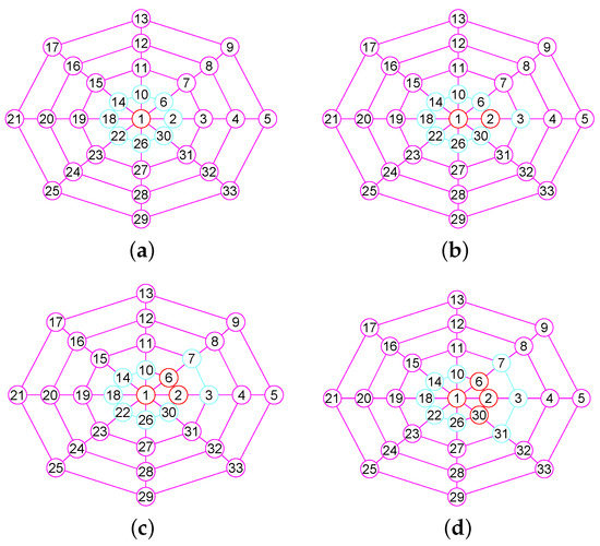
Figure 3. The 1-neighborhood subgraphs for the different nodes sets of a wheel graph G. (a) A wheel graph G and the 1-neighborhood subgraph $N\left(1\right)$ of the node 1; (b) The 1-neighborhood subgraph $N\left(S_1\right)$ of the nodes set $S_1=\{1,2\}$; (c) The 1-neighborhood subgraph $N\left(S_2\right)$ of the nodes set $S_2=\{1,2,6\}$; (d) The 1-neighborhood subgraph $N\left(S_3\right)$ of the nodes set $S_3=\{1,2,6,30\}$.

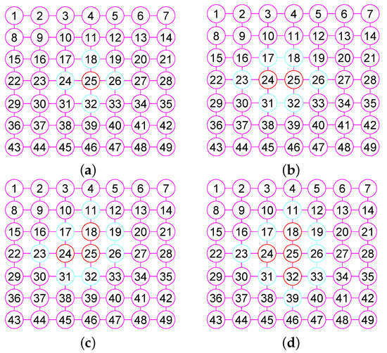
Figure 4. The 1-neighborhood subgraphs for the different nodes sets of the $7\times 7$ grid graph $G_{7,7}$. (a) A graph G and the 1-neighborhood subgraph $N\left(25\right)$ of the node 25; (b) The 1-neighborhood subgraph of the nodes set $S_1=\{24,25\}$; (c) The 1-neighborhood subgraph of the nodes set $S_2=\{24,25,18\}$; (d) The 1-neighborhood subgraph of the nodes set $S_3=\{24,25,18,32\}$.

For $Procedure$ 1, after computing $N\left(S_1\right)$, by Lemma 4, our algorithm orders all vertices of $N\left(S_1\right)$ into a sole linkage $L_1$ (observe Algorithm 1). For clarify, make $V_1=V\left(N\left(S_1\right)\right)$. If there are two vertices $v_i,v_j\in L_1$ meeting condition $v_i\asymp v_j$ concerning $N\left(S_1\right)$, then it proceeds to decide whether $v_i⪰v_j$ or $v_i\prec v_j$ concerning G. If $v_i⪰v_j$, it repositions $v_i$ in front of the $v_j$ in $L_1$. Otherwise, it repositions $v_i$ in back of the $v_j$ in $L_1$.

For every $Procedure$ r, $r=2,3,\cdots$, when computing $N\left(S_r\right)$, our algorithm successively calculates $V_2=V(N\left(S_{r-1}\right)\cap N\left(u_r\right))$ (see Figure 5d), $V_3=V(N\left(S_{r-1}\right)-N\left(u_r\right))$ (see Figure 5e), $V_4=V(N\left(u_r\right)-N\left(S_{r-1}\right))$ (see Figure 5f) and the degree sequences $d_{N\left(S_r\right)}$ $\left(V_1\right)$, $d_{N\left(S_r\right)}\left(V_3\right)$, $d_{N\left(S_r\right)}\left(V_4\right)$ in decreasing order respectively, where $S_{r-1}=\{u_1,u_2,\cdots$, $u_{r-1}\}$. It can be shown that $V_2\cup V_3\cup V_4=V\left(N\left(S_r\right)\right)$ and $V_i\cap V_j=\varnothing$ for $i\ne j,i,j=2,3,4$. By Lemma 4, it orders all vertices of $V_i$ into a sole linkage $L_i$ (observe Algorithm 1) for the neighborhood subgraph $N\left(S_r\right)$ with $i=2,3,4$, respectively.

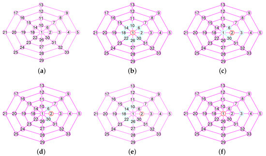
Figure 5. A wheel graph G, the 1-neighborhood subgraphs $N\left(1\right)$ and $N\left(2\right)$ and the three related vertices sets produced by the boolean operations of $N\left(1\right)$ and $N\left(2\right)$. (a) A wheel graph G; (b) The neighborhood subgraph $N\left(1\right)$; (c) The neighborhood subgraph $N\left(2\right)$; (d) $V\left(N\right(1\left)\right)\cap V\left(N\right(2\left)\right)=\{6,30\}$; (e) $V\left(N\right(1\left)\right)-V\left(N\right(2\left)\right)=\{10,14,18,$ $22,26\}$; (f) $V\left(N\right(2\left)\right)-V\left(N\right(1\left)\right)=$ $\left\{3\right\}$.

Next, our algorithm successively executes the following processing paces for the vertices of $L_i$ with $i=2,3,4$:

• Beginning from the front of $L_2$, it, in turn, decides whether every vertex $u\in L_2$ meets the $degree$ $multiplicity$ condition $d{m}_{N\left(S_r\right)}\left(u\right)$ $=1$. If the number of nodes meeting condition $d{m}_{N\left(S_r\right)}\left(u\right)$ $=1$ is less than 2 in $L_2$, it places u into $MaxQ\left(G\right)$. If there are two vertices $v_i,v_j\in L_2$ meeting condition $v_i\asymp v_j$ concerning $N\left(S_r\right)$, then it proceeds to decide whether $v_i⪰v_j$ or $v_i\prec v_j$ concerning G. If $v_i⪰v_j$, it repositions the $v_i$ in front of the $v_j$ in $L_2$ (observe Algorithm 1). Otherwise, it repositions the $v_i$ in back of the $v_j$ in $L_2$ (view Algorithm 1).
• Excluding the vertices added into $MaxQ\left(G\right)$, it utilizes a queue Q to save the middle vertices of $MaxQ\left(G\right)$. After executing Step 1, it consecutively decides whether or not each node $u\in L_2$ is in Q. If u is in Q and the number of vertices added into $MaxQ\left(G\right)$ is less than 2 in the previous process, it inserts u on the tail of $MaxQ\left(G\right)$ and concurrently deletes u from the head of Q. Otherwise, it places u on the back of Q.
• For $L_3$, if the number of nodes of $L_2$, added into $MaxQ\left(G\right)$, is 0 and the number of nodes meeting condition $d{m}_{N\left(S_r\right)}\left(u\right)$ $=1$ with $u\in L_3$ is less than 2, it inserts u on the back of $MaxQ\left(G\right)$. The remaining procedure steps are the same as for $L_2$.
• For $L_4$, if the number of nodes of $L_2$ and $L_3$, added into $MaxQ\left(G\right)$, is 0 and the number of nodes meeting the condition $d{m}_{N\left(S_r\right)}\left(u\right)$ $=1$ with $u\in L_4$ is less than 2, it places u on the back of $MaxQ\left(G\right)$. The remaining procedure steps are the same as for $L_2$.

Algorithm 1: Order all vertices of $V_i$ into a sole linkage $L_i$ for a neighborhood subgraph $N\left(S_r\right)$ with $i=1,2,3,4$, respectively where $V_1=V(N\left(S_1\right)$.

Algorithm 2: Contrast the $entire$ $diffusion$ $degree$ $sequences$ $d_H^{\sigma }\left[N_1\left(v\right)\right]$, $d_H^{\sigma }\left[N_2\left(v\right)\right]$, ⋯, $d_H^{\sigma }\left[N_{\rho \left(v\right)}\left(v\right)\right]$ and $d_H^{\sigma }\left[N_1\left(w\right)\right]$, $d_H^{\sigma }\left[N_2\left(w\right)\right]$, ⋯, $d_H^{\sigma }\left[N_{\rho \left(w\right)}\left(w\right)\right]$ of two vertices v and w in H.

Algorithm 3: Contrast two $diffusion$ $degree$ $sequences$ $d_{\sigma }\left(H_k\right)$ and $d_{\sigma }\left(J_k\right)$ of two vertices v and w in H.

Algorithm 4: Contrast $d_1$ and $d_2$.

Our algorithm utilizes an array $MaxQ$ to save the vertices of $MaxQ\left(G\right)$ and an array Q to store the vertices to be added to $MaxQ\left(G\right)$ briefly. Our algorithm has been optimized by Lemmas 2 and 3.

The results of experiments show that our method is a new approach by which one can precisely determine $TopMost$ graphs (defined in Section 2) for many classes of graphs, including trees, grid graphs, wheel graphs, hypercube graphs, king graphs, triangular graphs and so on. Figure 6, Figure 7, Figure 8, Figure 9, Figure 10, Figure 11, Figure 12, Figure 13, Figure 14, Figure 15, Figure 16, Figure 17, Figure 18, Figure 19, Figure 20, Figure 21, Figure 22 and Figure 23 given by our software display the accuracy of our software for computing $TopMost$ graphs of these graph classes aforesaid.

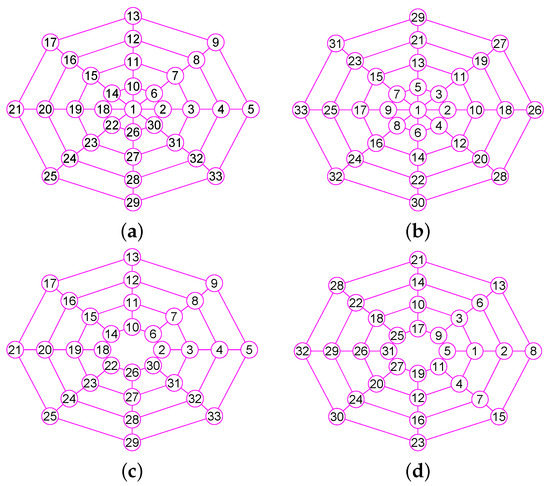
Figure 6. The $TopMost$ graphs of two graphs, including a wheel graph G and the graph $G-u$ with $u=1\in V\left(G\right)$. (a) A wheel graph G with 33 nodes and 64 edges; (b) The $TopMost$ graph of G; (c) The graph $G-u$ of 32 vertices and 56 edges; (d) The $TopMost$ graph of $G-u$.

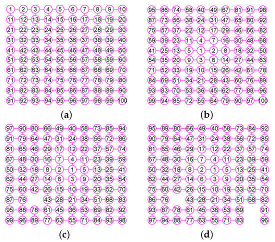
Figure 7. The $TopMost$ graphs of three graphs, including the $10\times 10$ grid graph $G_{10,10}$, $G_{10,10}-u$, $G_{10,10}-u-v-w$ with $u=73$, $v=88$, $w=97\in V\left(G_{10,10}\right)$. (a) A $10\times 10$ grid graph $G_{10,10}$ of 100 vertices and 180 edges; (b) The $TopMost$ graph of $G_{10,10}$; (c) The $TopMost$ graph of $G_{10,10}-u$; (d) The $TopMost$ graph of $G_{10,10}-u-v-w$.

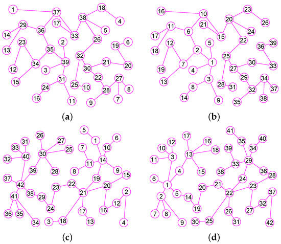
Figure 8. The $TopMost$ graphs of two trees $T_1$ and $T_2$. (a) A tree $T_1$ of 39 vertices and 38 edges; (b) The $TopMost$ graph of $T_1$; (c) A tree $T_2$ of 42 vertices and 41 edges; (d) The $TopMost$ graph of $T_2$.

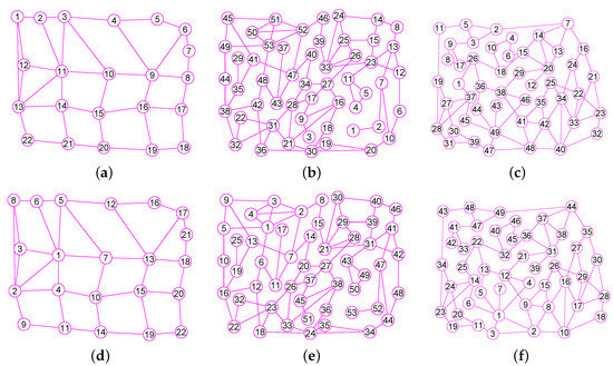
Figure 9. The $TopMost$ graphs of three graphs $G_1$, $G_2$ and $G_3$. (a) A graph $G_1$ of 22 vertices and 37 edges; (b) A graph $G_2$ of 53 vertices and 80 edges; (c) A graph $G_3$ of 49 vertices and 78 edges; (d) The $TopMost$ graph of $G_1$; (e) The $TopMost$ graph of $G_2$; (f) The $TopMost$ graph of $G_3$.

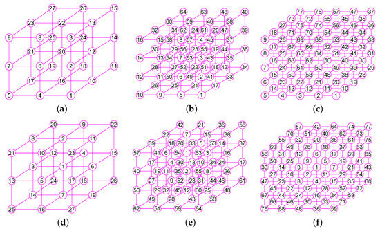
Figure 10. The $TopMost$ graphs of three graphs $G_{3,3,3}$, $G_{4,4,4}$ and $G_4$. (a) The $3\times 3\times 3$ grid graph $G_{3,3,3}$ of 27 vertices and 54 edges; (b) The $4\times 4\times 4$ grid graph $G_{4,4,4}$ of 64 vertices and 144 edges; (c) A graph $G_4$ of 77 vertices and 196 edges; (d) The $TopMost$ graph of $G_{3,3,3}$; (e) The $TopMost$ graph of $G_{4,4,4}$; (f) The $TopMost$ graph of $G_4$.

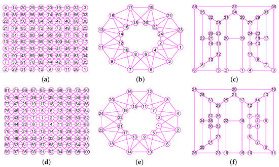
Figure 11. The $TopMost$ graphs of three graphs $G_5$, $G_6$ and $G_7$. (a) The $10\times 10$ king graph $G_5$ of 100 vertices and 342 edges; (b) The musical graph $G_6$ of 24 vertices and 60 edges; (c) The Barnette-Bosák-Lederberg graph $G_7$ of 38 vertices and 57 edges; (d) The $TopMost$ graph of $G_5$; (e) The $TopMost$ graph of $G_6$; (f) The $TopMost$ graph of $G_7$.

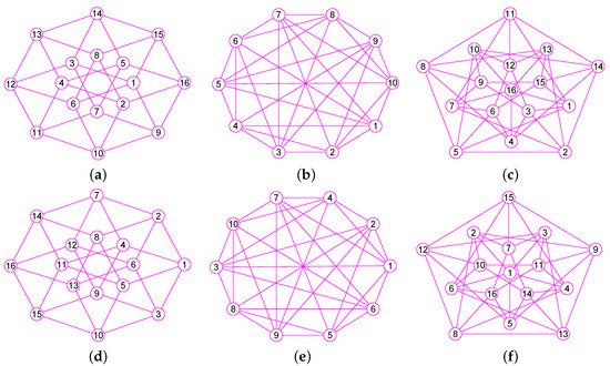
Figure 12. The $TopMost$ graphs of three regular graphs $G_8$, $G_9$ and $G_{10}$. (a) The 4-hypercube graph $G_8$ of 16 vertices and 32 edges; (b) The triangular graph $G_9$ of 10 vertices and 30 edges; (c) The Clebsch graph $G_{10}$ of 16 vertices and 40 edges; (d) The $TopMost$ graph of $G_8$; (e) The $TopMost$ graph of $G_9$; (f) The $TopMost$ graph of $G_{10}$.

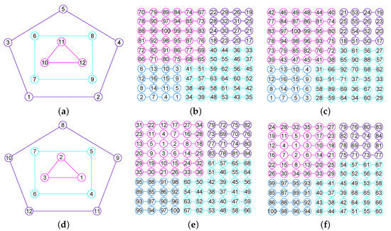
Figure 13. The $TopMost$ graphs of three unconnected graphs $G_{11}$, $G_{12}$ and $G_{13}$. (a) A disconnected graph $G_{11}$ with 12 nodes and 12 edges; (b) A disconnected graph $G_{12}$ that has four connected components and a total of 100 vertices and 160 edges; (c) A disconnected graph $G_{13}$ that has four connected components and a total of 100 vertices and 131 edges; (d) The $TopMost$ graph of $G_{11}$; (e) The $TopMost$ graph of $G_{12}$; (f) The $TopMost$ graph of $G_{13}$.

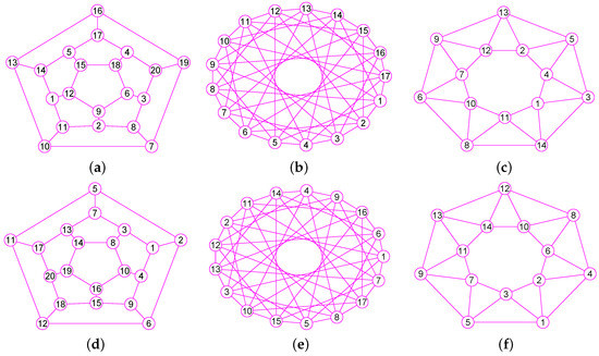
Figure 14. The $TopMost$ graphs of three graphs $G_{14}$, $G_{15}$ and $G_{16}$. (a) A Hamiltonian Graph $G_{14}$ of 20 vertices and 30 edges; (b) The 6-Andrásfai graph $G_{15}$ of 17 vertices and 51 edges; (c) The 7-antiprism graph $G_{16}$ of 14 vertices and 28 edges; (d) The $TopMost$ graph of $G_{14}$; (e) The $TopMost$ graph of $G_{15}$; (f) The $TopMost$ graph of $G_{16}$.

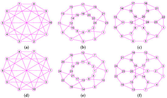
Figure 15. The $TopMost$ graphs of three graphs $K_{(5,5)}$, $G_{17}$ and $G_{18}$. (a) The complete bipartite graph $K_{(5,5)}$ of 10 vertices and 25 edges; (b) The 12-crossed prism graph $G_{17}$ of 24 vertices and 36 edges; (c) The 6th order cube-connected cycle graph $G_{18}$ of 24 nodes and 36 edges; (d) The $TopMost$ graph of $K_{(5,5)}$; (e) The $TopMost$ graph of $G_{17}$; (f) The $TopMost$ graph of $G_{18}$.

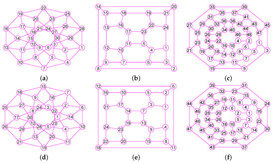
Figure 16. The $TopMost$ graphs of three graphs $G_{19}$, $G_{20}$ and $G_{21}$. (a) The Icosidodecahedral Graph $G_{19}$ with 30 nodes and 60 edges; (b) The truncated octahedron graph $G_{20}$ with 24 nodes and 36 edges; (c) The great rhombicuboctahedron graph $G_{21}$ of 48 nodes and 72 edges; (d) The $TopMost$ graph of $G_{19}$; (e) The $TopMost$ graph of $G_{20}$; (f) The $TopMost$ graph of $G_{21}$.

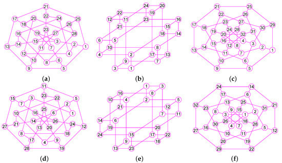
Figure 17. The $TopMost$ graphs of three graphs $G_{22}$, $G_{23}$ and $G_{24}$. (a) The coxeter graph $G_{22}$ of 28 vertices and 42 edges; (b) The Nauru graph $G_{23}$ with 24 nodes and 36 edges; (c) The Dyck graph $G_{24}$ of 32 nodes and 48 edges; (d) The $TopMost$ graph of $G_{22}$; (e) The $TopMost$ graph of $G_{23}$; (f) The $TopMost$ graph of $G_{24}$.

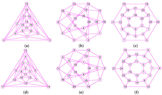
Figure 18. The $TopMost$ graphs of three graphs $G_{25}$, $G_{26}$ and $G_{27}$. (a) The Errera graph $G_{25}$ of 17 vertices and 45 edges; (b) The Folkman graph $G_{26}$ with 20 nodes and 40 edges; (c) A fullerene graph $G_{27}$ of 24 nodes and 36 edges; (d) The $TopMost$ graph of $G_{25}$; (e) The $TopMost$ graph of $G_{26}$; (f) The $TopMost$ graph of $G_{27}$.

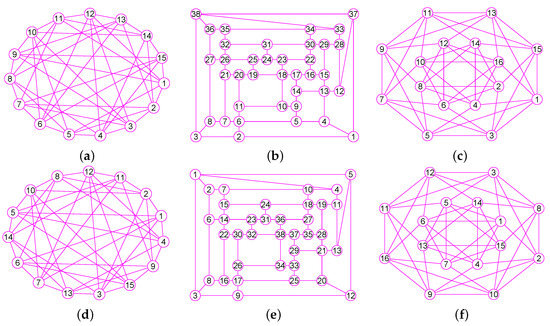
Figure 19. The $TopMost$ graphs of three graphs $G_{28}$, $G_{29}$ and $G_{30}$. (a) A generalized quadrangle graph $G_{28}$ with 15 nodes and 45 edges; (b) A pentagonal icositetrahedral graph $G_{29}$ with 38 nodes and 60 edges; (c) A Shrikhande graph $G_{30}$ of 16 nodes and 48 edges; (d) The $TopMost$ graph of $G_{28}$; (e) The $TopMost$ graph of $G_{29}$; (f) The $TopMost$ graph of $G_{30}$.

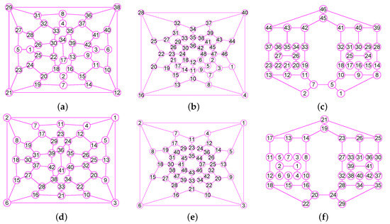
Figure 20. The $TopMost$ graphs of three graphs $G_{31}$, $G_{32}$ and $G_{33}$. (a) The Wiener-Araya graph $G_{31}$ of 42 vertices and 67 edges; (b) The Zamfirescu graph $G_{32}$ with 48 nodes and 76 edges; (c) The Faulkner-Younger graph $G_{33}$ of 42 nodes and 62 edges; (d) The $TopMost$ graph of $G_{31}$; (e) The $TopMost$ graph of $G_{32}$; (f) The $TopMost$ graph of $G_{33}$.

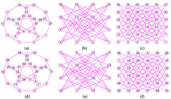
Figure 21. The $TopMost$ graphs of three graphs $G_{34}$, $G_{35}$ and $G_{36}$. (a) A triangle-replaced graph $G_{34}$ with 30 nodes and 45 edges; (b) The 4-dimensional Keller graph $G_{35}$ of 16 vertices and 46 edges; (c) The $6\times 6$ knight graph $G_{36}$ of 36 nodes and 80 edges; (d) The $TopMost$ graph of $G_{34}$; (e) The $TopMost$ graph of $G_{35}$; (f) The $TopMost$ graph of $G_{36}$.

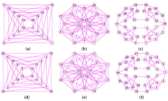
Figure 22. The $TopMost$ graphs of three graphs $G_{37}$, $G_{38}$ and $G_{39}$. (a) The Folkman graph $G_{37}$ of 20 vertices and 40 edges; (b) The 24-cell graph $G_{38}$ with 24 nodes and 96 edges; (c) The Thomassen graph $G_{39}$ of 34 nodes and 52 edges; (d) The $TopMost$ graph of $G_{37}$; (e) The $TopMost$ graph of $G_{38}$; (f) The $TopMost$ graph of $G_{39}$.

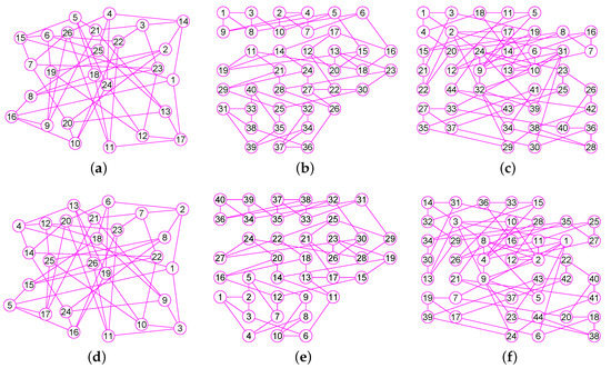
Figure 23. The $TopMost$ graphs of three graphs $G_{40}$, $G_{41}$ and $G_{42}$. (a) The projective plane graph $G_{40}$ of 26 vertices and 52 edges; (b) The Miyazaki graph $G_{41}$ with 40 nodes and 60 edges; (c) The Cubic Hypohamiltonian graph $G_{42}$ of 44 vertices and 75 edges; (d) The $TopMost$ graph of $G_{40}$; (e) The $TopMost$ graph of $G_{41}$; (f) The $TopMost$ graph of $G_{42}$.

5. Software Implementation

Utilizing the theory specified in the previous sections, we made a kit of software means called GraphLabel to calculate $canonical$ $labelings$ of graphs. Our experimental conditions included an Intel(R) Core(TM)2 Quad CPU Q6600 @2.40 GHz with 4.00 GB of RAM. The operating system was Microsoft Windows 8.1 Professional Edition. The graphics card was an NVIDIA GeForce 9800 GT. The display resolution was $1024\times 768\times 32$ bits (RGB). The internal hard drive was 500 GB. The programming environment was Microsoft Visual C++ 2012.

The software utilized object-oriented technique to construct many related classes, including $CNode$, $CNodeNeighbor$, $CEdge$, $CEdgeNeighbor$, $CGraph$ and so on. A complete explanation of the software functions is beyond the range of this paper. We will fully describe it in the other articles. All figures displayed in this article were created by employing our software system.

We chose a graph collection to check the correctness of our algorithms. We used our own software program to generate a large number of graphs randomly as the test cases, including Figure 7c,d, Figure 8, Figure 9 and Figure 10c. Besides, for enhancing the depth and breadth of experimentation, we also adopted many test cases from the online library [31] and library of benchmarks [32], including Figure 6, Figure 7a, Figure 10a,b, Figure 11, Figure 12, Figure 13, Figure 14, Figure 15, Figure 16, Figure 17, Figure 18, Figure 19, Figure 20, Figure 21, Figure 22 and Figure 23.

We applied our algorithms to as many classes of graphs as potential. These graphs presented here are only a small portion of the check graphs since the length of the paper is restricted. For comparing entirely, we offer both the initial and the resulting graph.

6. Summary and Future Work

In short, we get the following results: by Theorems 2–9, the paper has built a comparatively entire theoretical frame for computing the $canonical$ $labelings$ and $TopMost$ graphs of graphs. Algorithms 1–4 are unique and can correctly determine $TopMost$ graphs for many classes of graphs, including trees, grid graphs, wheel graphs, hypercube graphs, king graphs, triangular graphs and so on (see Figure 6, Figure 7, Figure 8, Figure 9, Figure 10, Figure 11, Figure 12, Figure 13, Figure 14, Figure 15, Figure 16, Figure 17, Figure 18, Figure 19, Figure 20, Figure 21, Figure 22 and Figure 23). Algorithms 1–4 are also valid for detached undirected graphs. For every vertex in a graph G, the definition of the property $m\_NearestNode$ enhances the accuracy of computing $canonical$ $labeling$. By software evaluating, the accuracy of our algorithms is elementarily established. Our approach can be employed to excavate the frequent subgraph. Additionally, it proposes Conjecture 1.

Nevertheless, there are still many aspects we need to progress, including verifying the conjectures suggested by us, improving our software platform and employing more test cases to check our program. Specifically, we need to reinforce our algorithms so that they can determine the $canonical$ $labelings$ for more classes of graphs.

Currently, we are considering how to stretch our method to dig the frequent subgraphs and determine the $canonical$ $labelings$ of weighted graphs. We will present further research in other papers.

References

- Hao, J.; Gong, Y.; Wang, Y.; Tan, L.; Sun, J. Using k-Mix-Neighborhood Subdigraphs to Compute Canonical Labelings of Digraphs. Entropy 2017, 19, 79. [Google Scholar] [CrossRef]
- Hao, J.; Gong, Y.; Tan, L.; Duan, D. Apply Partition Tree to Compute Canonical Labelings of Graphs. Int. J. Grid Distrib. Comput. 2016, 9, 241–264. [Google Scholar]
- McKay, B. Computing Automorphisms and Canonical Labellings of Graphs Combinatorial Mathematics; Lecture Notes in Mathematics; Springer: Berlin/Heidelberg, Germany, 1978; Volume 686, pp. 223–232. [Google Scholar]
- Piperno, A. Search space contraction in canonical labeling of graphs. arxiv 2008, arXiv:0804.4881. [Google Scholar]
- Junttila, T.; Kaski, P. Engineering an Efficient Canonical Labeling Tool for Large and Sparse Graphs. In Proceedings of the Ninth Workshop on Algorithm Engineering and Experiments and the Fourth Workshop on Analytic Algorithmics and Combinatorics, New Orleans, LA, USA, 6 January 2007; Siam: Philadelphia, PA, USA, 2007; pp. 135–149. [Google Scholar]
- Shah, Y.J.; Davida, G.I.; McCarthy, M.K. Optimum Featurs and Graph Isomorphism. IEEE Trans. Syst. Man Cybern. 1974, SMC-4, 313–319. [Google Scholar] [CrossRef]
- Ivanciuc, O. Canonical Numbering and Constitutional Symmetry. In Handbook of Chemoinformatics; Wiley-VCH Verlag GmbH: Weinheim, Germany, 2008; pp. 139–160. [Google Scholar]
- Babai, L.; Luks, E.M. Canonical Labeling of Graphs. In Proceedings of the Fifteenth Annual ACM Symposium on Theory of Computing, Boston, MA, USA, 25–27 April 1983; ACM: New York, NY, USA, 1983; pp. 171–183. [Google Scholar] [CrossRef]
- Jantschi, L.; Bolboaca, S.D. Conformational study of C-24 cyclic polyyne clusters. Int. J. Quantum Chem. 2018, 118, e25614. [Google Scholar] [CrossRef]
- Joiţa, D.M.; Jäntschi, L. Extending the Characteristic Polynomial for Characterization of C20 Fullerene Congeners. Mathematics 2017, 5, 84. [Google Scholar] [CrossRef]
- Bolboaca, S.; Jantschi, L. How good can the characteristic polynomial be for correlations? Int. J. Mol. Sci. 2007, 8, 335–345. [Google Scholar] [CrossRef]
- Kuramochi, M.; Karypis, G. Finding Frequent Patterns in a Large Sparse Graph*. Data Min. Knowl. Discov. 2005, 11, 243–271. [Google Scholar] [CrossRef]
- Kuramochi, M.; Karypis, G. An efficient algorithm for discovering frequent subgraphs. IEEE Trans. Knowl. Data Eng. 2004, 16, 1038–1051. [Google Scholar] [CrossRef]
- Huan, J.; Wang, W.; Prins, J. Efficient mining of frequent subgraphs in the presence of isomorphism. In Proceedings of the Third IEEE International Conference on Data Mining, Melbourne, FL, USA, 22 November 2003; pp. 549–552. [Google Scholar]
- Kashani, Z.; Ahrabian, H.; Elahi, E.; Nowzari-Dalini, A.; Ansari, E.; Asadi, S.; Mohammadi, S.; Schreiber, F.; Masoudi-Nejad, A. Kavosh: A new algorithm for finding network motifs. BMC Bioinform. 2009, 10, 318. [Google Scholar] [CrossRef] [PubMed]
- He, P.R.; Zhang, W.J.; Li, Q. Some further development on the eigensystem approach for graph isomorphism detection. J. Frankl. Inst.-Eng. Appl. Math. 2005, 342, 657–673. [Google Scholar] [CrossRef]
- Arvind, V.; Das, B.; Köbler, J. A Logspace Algorithm for Partial 2-Tree Canonization. In Computer Science-Theory and Applications; Springer: Berlin/Heidelberg, Germany, 2008; Volume 5010, pp. 40–51. [Google Scholar] [CrossRef]
- Babai, L.; Kucera, L. Canonical labelling of graphs in linear average time. In Proceedings of the 20th Annual Symposium on Foundations of Computer Science, San Juan, Puerto Rico, 29–31 October 1979; pp. 39–46. [Google Scholar] [CrossRef]
- Arnborg, S.; Proskurowski, A. Canonical Representations of Partial 2- and 3-Trees. In Proceedings of the 2nd Scandinavian Workshop on Algorithm Theory, Bergen, Norway, 11–14 July 1990; Lecture Notes in Computer Science 477. Springer: Berlin, Germany, 1990; pp. 197–214. [Google Scholar]
- McKay, B. Practical Graph Isomorphism; Department of Computer Science, Vanderbilt University: Nashville, TN, USA, 1981. [Google Scholar]
- McKay, B.D. Isomorph-Free Exhaustive Generation. J. Algorithms 1998, 26, 306–324. [Google Scholar] [CrossRef]
- Practical graph isomorphism, {II}. J. Symb. Comput. 2014, 60, 94–112. [CrossRef]
- Yan, X.; Han, J. gSpan: Graph-based substructure pattern mining. In Proceedings of the 2002 IEEE International Conference on Data Mining, ICDM 2003, Maebashi City, Japan, 9–12 December 2002; pp. 721–724. [Google Scholar] [CrossRef]
- Miyazaki, T. The Complexity of McKay’s Canonical Labeling Algorithm; Citeseer: University Park, PA, USA, 1997. [Google Scholar]
- Tener, G.; Deo, N. Efficient isomorphism of miyazaki graphs. Algorithms 2008, 5, 7. [Google Scholar]
- Junttila, T.; Kaski, P. Conflict Propagation and Component Recursion for Canonical Labeling Theory and Practice of Algorithms in (Computer) Systems; Lecture Notes in Computer Science; Springer: Berlin/Heidelberg, Germany, 2011; Volume 6595, pp. 151–162. [Google Scholar]
- López-Presa, J.L.; Anta, A.F.; Chiroque, L.N. Conauto-2.0: Fast Isomorphism Testing and Automorphism Group Computation. arXiv 2011, arXiv:1108.1060. [Google Scholar]
- Katebi, H.; Sakallah, K.; Markov, I. Graph Symmetry Detection and Canonical Labeling: Differences and Synergies. arXiv 2012, arXiv:1208.6271. [Google Scholar]
- Habtemicael, S.; SenGupta, I. Pricing variance and volatility swaps for Barndorff-Nielsen and Shephard process driven financial markets. Int. J. Financ. Eng. 2016, 3, 1650027. [Google Scholar] [CrossRef]
- Mariani, M.C.; SenGupta, I.; Bezdek, P. Numerical solutions for option pricing models including transaction costs and stochastic volatility. Acta Appl. Math. 2012, 118, 203–220. [Google Scholar] [CrossRef]
- Weisstein, E.W. Simple Graphs–from Wolfram MathWorld; Wolfram Research: Champaign, IL, USA, 2015. [Google Scholar]
- ALENEX 2007 Submission: Source Code, Benchmark Instances, and Summary Results. Available online: http://www.tcs.hut.fi/Software/benchmarks/ALENEX-2007/ (accessed on 30 June 2018).
© 2019 by the authors. Licensee MDPI, Basel, Switzerland. This article is an open access article distributed under the terms and conditions of the Creative Commons Attribution (CC BY) license (http://creativecommons.org/licenses/by/4.0/).