Iterative Methods with Memory for Solving Systems of Nonlinear Equations Using a Second Order Approximation

Abstract

Iterative methods for solving nonlinear equations are said to have memory when the calculation of the next iterate requires the use of more than one previous iteration. Methods with memory usually have a very stable behavior in the sense of the wideness of the set of convergent initial estimations. With the right choice of parameters, iterative methods without memory can increase their order of convergence significantly, becoming schemes with memory. In this work, starting from a simple method without memory, we increase its order of convergence without adding new functional evaluations by approximating the accelerating parameter with Newton interpolation polynomials of degree one and two. Using this technique in the multidimensional case, we extend the proposed method to systems of nonlinear equations. Numerical tests are presented to verify the theoretical results and a study of the dynamics of the method is applied to different problems to show its stability.

1. Introduction

This paper deals with iterative methods for approximating the solutions of a nonlinear system of n equations and n unknowns, $F\left(x\right)=0$, where $F:D\subseteq {\mathbb{R}}^n⟶{\mathbb{R}}^n$ is a nonlinear vectorial function defined in a convex set D. The main aim of this work is to design iterative methods with memory for approximating the solutions $\xi$ of $F\left(x\right)=0$. An iterative method is said to have memory when the fixed point function G depends on more than one previous iteration, that is, the iterative expression is $x_{k+1}=G(x_k,x_{k-1},\cdots )$.

A classical iterative scheme with memory for solving scalar equations $f\left(x\right)=0$, $n=1$, is the known secant method, whose iterative expression is

$$x_{k+1}=x_k-{\displaystyle \frac{f\left(x_k\right)(x_k-x_{k-1})}{f\left(x_k\right)-f\left(x_{k-1}\right)}},k=1,2,\dots ,$$

(1)

with $x_0$ and $x_1$ as initial estimations. This method can be obtained from Newton’s scheme by replacing the derivative by the first divided difference $f[x_k,x_{k-1}]$. For $n>1$ the secant method has the expression

$$x^{(k+1)}=x^{\left(k\right)}-{[x^{\left(k\right)},x^{(k-1)};F]}^{-1}F\left(x^{\left(k\right)}\right),k=1,2,\dots ,$$

(2)

where $[x^{\left(k\right)},x^{(k-1)};F]$ is the divided difference operator, defined in [1].

It is possible to design methods with memory starting from methods without memory by introducing accelerating parameters. The idea is to introduce parameters in the original scheme and study the error equation of the method to see if any particular values of these parameters allow to increase the order of convergence, see for example [2,3,4] and the references therein. Several authors have constructed iterative methods with memory for solving nonlinear systems, by approximating the accelerating parameters by Newton’s polynomial interpolation of first degree, see for example the results presented by Petković and Sharma in [5] and by Narang et al. in [6]. As far as we know, in the multivariate case, higher-degree Newton polynomials have never been used. In this paper, we will approximate the accelerating parameters with multidimensional Newton’s polynomial interpolation of second degree.

In [1], Ortega and Rheinboldt introduced a general definition of the order of convergence, called R-order defined as follows

$$R_p\left\{x_k\right\}=\left\{\begin{array}{c}{\displaystyle \underset{k\to \infty }{lim}sup{\left(e_k\right)}^{\frac{1}{k}},ifp=1}\\ {\displaystyle \underset{k\to \infty }{lim}sup{\left(e_k\right)}^{\frac{1}{p^k}},ifp>1}\end{array}\right.$$

(3)

where $e_k=x_k-\xi$, $k=0,1,\dots$, and $R_p$ is called R-factor. The R-order of convergence of an iterative method (IM) at the point $\xi$ is

$$O_R(\left(IM\right),\xi )=\left\{\begin{array}{c}+\infty ,\mathrm{if}{R}_m(\left(IM\right),\xi )=0,\mathrm{for}\mathrm{all}m\in [1,+\infty )\hfill \\ inf\{m\in [1,+\infty ):R_m(\left(IM\right),\xi )=1\},\mathrm{otherwise}\hfill \end{array}\right.$$

(4)

Let (IM) be an iterative method with memory that generates a sequence $\left\{x_k\right\}$ of approximations to the root $\xi$, and let us also assume that this sequence converges to $\xi$. If there exists a nonzero constant $\eta$ and nonnegative numbers $t_i$, $0\le i\le m$ such that the inequality

$$|e_{k+1}|\le \eta \prod _{i=0}^m{|e_{k-i}|}^{t_i}$$

(5)

holds, then the R-order of convergence of (IM) satisfies the inequality

$$O_R(\left(IM\right),\xi )\ge s^{*},$$

(6)

where $s^{*}$ is the unique positive root of the equation

$$s^{m+1}-\sum _{i=0}^m{t}_i{s}^{m-i}=0.$$

(7)

We can find the proof of this result in [1].

Now, we introduce some notations that we use in this manuscript. Let r be the order of an iterative method, then

$$e_{k+1}\sim D_{k,r}{e}_k^r,$$

(8)

where $D_{k,r}$ tends to the asymptotic error constant of the iterative method when $k\to \infty$. To avoid higher order terms in the Taylor series that do not influence the convergence order, we will use the notation used by Traub in [2]. If $\left\{f_k\right\}$ and $\left\{g_k\right\}$ are null sequences (that is, sequences convergent to zero) and

$$\frac{f_k}{g_k}\to C,$$

(9)

where C is a nonzero constant, we can write

$$f_k=\mathcal{O}\left(g_k\right)\mathrm{or}{f}_k\sim C{g}_k.$$

(10)

Let ${\left\{x^{\left(k\right)}\right\}}_{k\ge 0}$ be a sequence of vectors generated by an iterative method converging to a zero of F, with R-order greater than or equal to r, then according to [4] we can write

$$e_{k+1}\sim D^{(k,r)}{\left(e_k\right)}^r,$$

(11)

where $\left\{D^{(k,r)}\right\}$ is a sequence which tends to the asymptotic error constant $D^r$ of the iterative method when $k\to \infty$, so $e_{k+1}\sim e_k$.

Accelerating Parameters

We illustrate the technique of the accelerating parameters, introduced by Traub in [2], starting from a very simple method with a real parameter $\alpha$

$$x_{k+1}=x_k-\alpha f\left(x_k\right),k=1,2,\cdots$$

(12)

This method has first order of convergence, with error equation

$$e_{k+1}=(1-\alpha f^{\prime }\left(\xi \right))e_k+\mathcal{O}\left[e_k^2\right],$$

(13)

where $e_k=x_k-\xi$, $k=0,1,\dots$

As it is easy to observe, the order of convergence can increase up to 2 if $\alpha ={\displaystyle \frac{1}{f^{\prime }\left(\xi \right)}}$. Since $\xi$ is unknown, we estimate $f^{\prime }\left(\xi \right)$ by approximating the nonlinear function with a Newton polynomial interpolation of degree 1, at points $(x_k,f\left(x_k\right))$ and $(x_{k-1},f\left(x_{k-1}\right))$

$$N_1\left(t\right)=f\left(x_{k-1}\right)+f[x_k,x_{k-1}](t-x_{k-1})=f\left(x_{k-1}\right)+{\displaystyle \frac{f\left(x_k\right)-f\left(x_{k-1}\right)}{x_k-x_{k-1}}}(t-x_{k-1}).$$

(14)

To construct the polynomial $N_1\left(t\right)$, it is necessary to evaluate the nonlinear function f in two points; so, two initial estimates are required, $x_1$ and $x_0$. The derivative of the nonlinear function is approximated by the derivative of the interpolating polynomial, that is, $\alpha ={\displaystyle \frac{1}{f^{\prime }\left(\xi \right)}}\approx {\displaystyle \frac{1}{N_1^{\prime }\left(x_k\right)}}$, and the resulting scheme is

$$\begin{array}{ccc}\hfill {\alpha }_k& =& {\displaystyle \frac{x_k-x_{k-1}}{f\left(x_k\right)-f\left(x_{k-1}\right)}},\hfill \\ \hfill x_{k+1}& =& x_k-{\alpha }_{k}f\left(x_k\right),\hfill \end{array}$$

(15)

substituting ${\alpha }_k$ in the iterative expression

$$x_{k+1}=x_k-{\displaystyle \frac{f\left(x_k\right)(x_k-x_{k-1})}{f\left(x_k\right)-f\left(x_{k-1}\right)}},$$

(16)

we get the secant method [7], with order of convergence $p={\displaystyle \frac{1+\sqrt{5}}{2}}\approx 1.6180$.

2. Modified Secant Method

A similar process can be done now using a Newton polynomial interpolation of second degree for approximating parameter $\alpha$. As it is a better approximation of the nonlinear function, it is expected that the order of convergence of the resulting scheme is greater than the obtained in the case of a polynomial of degree 1. For the modified secant method, the approximation of the parameter is ${\alpha }_k\approx {\displaystyle \frac{1}{N_2^{\prime }\left(x_k\right)}}$, where

$$N_2\left(t\right)=f\left(x_{k-1}\right)+f[x_k,x_{k-1}](t-x_{k-1})+f[x_k,x_{k-1},x_{k-2}](t-x_k)(t-x_{k-1}),$$

(17)

being

$$f[x_k,x_{k-1},x_{k-2}]={\displaystyle \frac{f[x_k,x_{k-1}]-f[x_{k-1},x_{k-2}]}{x_k-x_{k-2}}}.$$

(18)

So,

$$N_2^{\prime }\left(x_k\right)=f[x_k,x_{k-1}]+f[x_k,x_{k-1},x_{k-2}](2t-x_k-x_{k-1})$$

and replacing this expression in ${\alpha }_k={\displaystyle \frac{1}{N_2^{\prime }\left(x_k\right)}}$ an iterative method with memory is obtained

$$\begin{array}{ccc}\hfill {\alpha }_k& =& \frac{1}{{\displaystyle \frac{x_k(f\left(x_{k-1}\right)-f\left(x_{k-2}\right))+x_{k-1}(f\left(x_{k-2}\right)-f\left(x_k\right))+x_{k-2}(f\left(x_k\right)-f\left(x_{k-1}\right))}{(x_k-x_{k-2})(x_{k-2}-x_{k-1})}}+f[x_k,x_{k-1}]},\hfill \\ \hfill x_{k+1}& =& x_k-{\alpha }_{k}f\left(x_k\right).\hfill \end{array}$$

(19)

Now, three initial points are necessary, $x_k$, $x_{k-1}$ and $x_{k-2}$, to calculate the value of parameter ${\alpha }_k$.

In the following result, we present the order of convergence of the iterative scheme with memory (19).

Theorem 1.

(Order of convergence of the modified secant method) Let ξ be a simple zero of a sufficiently differentiable function $f:D\subseteq \mathbb{R}⟶\mathbb{R}$ in an open interval D. Let $x_0$, $x_1$ and $x_2$ be initial guesses sufficiently close to ξ. Then, the order of convergence of method (19) is at least $1.8393$, with error equation $e_{k+1}\sim c_3{e}_{k-1}{e}_{k-2}{e}_k$.

Proof. 

By substituting the different terms of ${\alpha }_k$ by their Taylor expansions, we have

$$(1-{\alpha }_k{f}^{\prime }\left(\xi \right))\sim c_3{e}_{k-1}{e}_{k-2}.$$

Now, from the error Equation (13)

$$e_{k+1}\sim c_3{e}_{k-1}{e}_{k-2}{e}_k.$$

(20)

By Writing $e_k$ and $e_{k-1}$ in terms of $e_{k-2}$, we obtain

$$e_{k+1}\sim e_{k-2}{e}_{k-2}^p{e}_{k-2}^{p^2}=e_{k-2}^{p^2+p+1}.$$

(21)

where p denotes the order of convergence of method (19). But, if p is the order of (19), then $e_{k+1}\sim e_{k-2}^{p^3}$. Therefore, p must satisfy $p^3=p^2+p+1$. The unique positive root of this cubic polynomial is $p\approx 1.8393$ and, by applying the result of Ortega and Rheinbolt, this is the order of convergence of scheme (19). □

The efficiency index, defined by Ostrowski in [8], depends on the number of functional evaluations per iteration, d, and on the order of convergence p, in the way

$$I=p^{1/d},$$

(22)

so, as in the modified secant method there is only one new functional evaluation per iteration, its efficiency index is $1.8393$.

Nonlinear Systems

Method (12) can be extended for approximating the roots of a nonlinear system $F\left(x\right)=0$, where $F:D\subseteq {\mathbb{R}}^n⟶{\mathbb{R}}^n$ is a vectorial function defined in a convex set D,

$$x^{(k+1)}=x^{\left(k\right)}-\alpha F\left(x^{\left(k\right)}\right).$$

(23)

It is easy to prove that this method has linear convergence, with error equation

$$e_{k+1}=(1+\alpha F^{\prime }\left(\xi \right))e_k+\mathcal{O}\left[e_k^2\right],$$

(24)

being $e_k=x^{\left(k\right)}-\xi$, $k=0,1,\dots$

In the multidimensional case, we can approximate the parameter $\alpha ={\left[F^{\prime }\left(\xi \right)\right]}^{-1}$ with a multivariate Newton polynomial interpolation. If we use a polynomial of first degree

$$N_1\left(t\right)=F\left(x^{(k-1)}\right)+[x^{\left(k\right)},x^{(k-1)};F](t-x^{(k-1)}),$$

(25)

then $N_1^{\prime }\left(x^{\left(k\right)}\right)=[x^{\left(k\right)},x^{(k-1)},F]$ and $\alpha$ is approximated by ${\alpha }_k={[x^{\left(k\right)},x^{(k-1)};F]}^{-1}$, so the iterative resulting method is

$$x^{(k+1)}=x^{\left(k\right)}-{[x^{\left(k\right)},x^{(k-1)};F]}^{-1}F\left(x^{\left(k\right)}\right),$$

(26)

that corresponds to the secant method for the multidimensional case.

To extend the modified secant method (19) to this context, we need a multidimensional Newton polynomial interpolation of second degree

$$N_2\left(t\right)=F\left(x^{(k-1)}\right)+[x^{\left(k\right)},x^{(k-1)};F](t-x^{(k-1)})+[x^{\left(k\right)},x^{(k-1)},x^{(k-2)};F](t-x^{\left(k\right)})(t-x^{(k-1)}),$$

(27)

where

$$[·,·,·;F]:{\mathbb{R}}^n\times {\mathbb{R}}^n\times {\mathbb{R}}^n\to \mathcal{B}({\mathbb{R}}^n\times {\mathbb{R}}^n,{\mathbb{R}}^n),$$

(28)

such that $[x,y,z;F](x-z)=[x,y;F]-[y,z;F]$, where $\mathcal{B}$ denotes the set of bi-linear mappings.

Moreover,

$$N_2^{\prime }\left(t\right)=[x^{\left(k\right)},x^{(k-1)};F]+[x^{\left(k\right)},x^{(k-1)},x^{(k-2)};F]((t-x^{\left(k\right)})+(t-x^{(k-1)})),$$

(29)

evaluating the derivative in $x^{\left(k\right)}$,

$$N_2^{\prime }\left(x^{\left(k\right)}\right)=[x^{\left(k\right)},x^{(k-1)};F]+[x^{\left(k\right)},x^{(k-1)},x^{(k-2)};F](x^{\left(k\right)}-x^{(k-1)}).$$

(30)

So, the iterative expression of the resulting method with memory is

$$x^{(k+1)}=x^{\left(k\right)}-{[[x^{\left(k\right)},x^{(k-1)};F]+[x^{\left(k\right)},x^{(k-1)},x^{(k-2)};F](x^{\left(k\right)}-x^{(k-1)})]}^{-1}F\left(x^{\left(k\right)}\right),k=2,3,\dots$$

(31)

The divided difference operator can be expressed in its integral form by using the Genocchi-Hermite formula for divided difference of first order [9]

$$[x,x+h;F]={\int }_0^1{F}^{\prime }(x+ht)dt,$$

(32)

as

$$F^{\prime }(x+ht)=F^{\prime }\left(x\right)+F^{″}\left(x\right)ht+\frac{1}{2}{F}^{‴}\left(x\right){\left(ht\right)}^2+\cdots ,$$

(33)

then

$$[x,x+h;F]=F^{\prime }\left(x\right)+\frac{h}{2}{F}^{″}\left(x\right)+\frac{h^2}{6}{F}^{‴}\left(x\right)+\cdots ,$$

(34)

and, in general, the divided difference of k-order can be calculated by [10]

$$[x_0,x_1,\cdots ,x_k;F]={\int }_0^1\cdots {\int }_0^1{t}_1^{k-1}{t}_2^{k-2}\cdots t_{k-1}{F}^{\left(k\right)}\left(\mu \right)d{t}_{1}d{t}_2\cdots d{t}_k,$$

(35)

where

$$\mu =x_0+t_1(x_1-x_0)+t_1{t}_2(x_2-x_1)+\cdots +t_1{t}_2\cdots t_k(x_k-x_{k-1}).$$

(36)

Theorem 2.

(Order of Convergence of the Modified Secant Method in the Multidimensional Case) Let ξ be a zero of a sufficiently differentiable function $F:D\subseteq {\mathbb{R}}^n⟶{\mathbb{R}}^n$ in a convex set D, such that $F^{\prime }\left(\xi \right)$ is nonsingular. Let $x^{\left(0\right)}$, $x^{\left(1\right)}$ and $x^{\left(2\right)}$ be initial guesses sufficiently close to ξ. Then the order of convergence of que method (31) is at least 1.8393 with error equation

$$e_{k+1}\sim c_3{e}_{k-1}{e}_{k-2}{e}_k,$$

being $c_k=(1/k!){\left[F^{\prime }\left(\xi \right)\right]}^{-1}{F}^{\left(k\right)}\left(\xi \right),k=2,3,\dots$

Proof. 

For the second order divided difference we write (35) for $k=2$ in the following way

$$\begin{array}{ccc}\hfill [x,x+h,x+k;F]& =& {\int }_0^1{\int }_0^1{F}^{″}(x+h{t}_1+k{t}_2)d{t}_{1}d{t}_2\hfill \\ & =& {\displaystyle \frac{1}{2}}{F}^{″}\left(x\right)+{\displaystyle \frac{1}{3}}{F}^{‴}\left(x\right)\left(h+\frac{k}{2}\right)+\frac{1}{8}{F}^{\left(iv\right)}\left(x\right)\left(h^2+\frac{k^2}{3}+hk\right),\hfill \end{array}$$

(37)

where $h=x_k-x_{k-1}$ and $k=x_{k-2}-x_{k-1}$. We can write h and k in terms of the errors as $h=e_k-e_{k-1}$ and $k=e_{k-2}-e_{k-1}$. Substituting the approximation of $\alpha$, ${\alpha }_k$, in the error equation (24), we obtain

$$e_{k+1}\sim c_3{e}_{k-1}{e}_{k-2}{e}_k.$$

(38)

Following the same steps as in the unidimensional case, the order of convergence p of method (31) must satisfy the equation $p^3=p^2+p+1$, which has the unique positive root $p=1.8393$. □

3. Dynamical and Numerical Study

When a new method is designed, it is interesting to analyze the dynamical behavior of the rational function that appears when the scheme is applied on polynomials of low degree. For the secant method, this analysis has been made by different researchers, so we are going to study the behavior of the modified secant method. As this scheme would be accurate for quadratic polynomials, due to the approximation we make, we use 3rd degree polynomials in this analysis. In order to make a general study, we use four polynomials that combined can generate any third degree polynomial, that is, $p_1\left(x\right)=x^3-x$, $p_2\left(x\right)=x^3+x$, $p_3\left(x\right)=x^3$ and $p_4\left(x\right)=x^3+\gamma x+1$, where $\gamma$ is a free real parameter.

The rational operators obtained when our method (31) is applied on the mentioned polynomials are:

$$\begin{array}{ccc}\hfill O_{p_1}(x_{k-2},x_{k-1},x_k)& =& -{\displaystyle \frac{x_k\left(5x_k^2-x_{k-1}^2-x_{k-1}{x}_{k-2}-x_{k-2}^2\right)}{-6x_k^2+x_{k-1}^2+x_{k-1}{x}_{k-2}+x_{k-2}^2+1}},\hfill \\ \hfill O_{p_2}(x_{k-2},x_{k-1},x_k)& =& -{\displaystyle \frac{x_k\left(5x_k^2-x_{k-1}^2-x_{k-1}{x}_{k-2}-x_{k-2}^2\right)}{-6x_k^2+x_{k-1}^2+x_{k-1}{x}_{k-2}+x_{k-2}^2-1}},\hfill \\ \hfill O_{p_3}(x_{k-2},x_{k-1},x_k)& =& -{\displaystyle \frac{x_k\left(5x_k^2-x_{k-1}^2-x_{k-1}{x}_{k-2}-x_{k-2}^2\right)}{-6x_k^2+x_{k-1}^2+x_{k-1}{x}_{k-2}+x_{k-2}^2}},\hfill \\ \hfill O_{p_4}(x_{k-2},x_{k-1},x_k)& =& -{\displaystyle \frac{5x_k^3-x_k\left(x_{k-1}^2+x_{k-1}{x}_{k-2}+x_{k-2}^2\right)-1}{-\gamma -6x_k^2+x_{k-1}^2+x_{k-1}{x}_{k-2}+x_{k-2}^2}}.\hfill \end{array}$$

In order to analyze the fixed points, we introduce the auxiliary operators $G_i$, $i=1,2,3,4$, defined as follows

$$G_i(x_{k-2},x_{k-1},x_k)=(x_{k-1},x_k,O_{p_i}(x_{k-2},x_{k-1},x_k)),i=1,2,3,4.$$

So, a point $(x_{k-2},x_{k-1},x_k)$ is a fixed point of $G_i$ if $x_{k-2}=x_{k-1}$, $x_{k-1}=x_k$ and $x_k=O_{p_i}(x_{k-2},x_{k-1},x_k)$. We can prove that there are no fixed points different from the roots of the polynomials. So, the method is very stable. On the other hand, critical points are also interesting because a classical result of Fatou and Julia states that each basin of attraction of an attracting fixed point contains at least a critical point ([11,12]), so it is important to determine to which basin of attraction belongs each critical point. The critical points are determined by the calculation of the determinant of the Jacobian matrix $G_i^{\prime }$, $i=1,2,3,4$ ([13]). For the polynomials $p_1$ to $p_4$ the critical points are the roots of the polynomials and the points $(x_{k-2},x_{k-1},x_k)$, such that $x_{k-1}=-2x_{k-2}$.

The bifurcation diagram ([13]) is a dynamical tool that shows the behavior of the sequence of iterates depending on a parameter. In this case, we use parameter $\gamma$ from $p_4\left(x\right)$. Starting from an initial estimation close to zero, we use a mesh of 500 subintervals for $\gamma$ in the x axis and we draw the last 100 iterates. In Figure 1a, we plot the real roots of $p_4$ and in Figure 1b we draw the bifurcation diagram. We can see how the bifurcation diagram always matches the solutions.

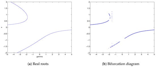
Figure 1. Comparison between the real roots and the iterative method.

Now, we are going to compare Newton’s method and the secant and modified secant schemes on the following test functions, under different numerical characteristics, as well as the dynamical planes associated to them.

(1)

$f_1\left(x\right)=sin\left(x\right)-x^2+1$,

(2)

$f_2\left(x\right)=(x-1)(x^3+x^{10}+1)sin\left(x\right)$,

(3)

$f_3\left(x\right)=arctan\left(x\right)$,

(4)

$F_4(x_1,x_2)=(x_1^2-1,x_2^2-1)$,

(5)

$F_5(x_1,x_2)=(x_1^2-x_1-x_2^2-1,x_2-sin\left(x_1\right))$,

(6)

$F_6(x_1,x_2,x_3)=(x_{1}x-2-1,x_{2}x-3-1,x_{1}x-3-1)$.

Variable precision arithmetics has been used with 100 digits of mantissa, with the stopping criterion $|x_{k+1}-x_k|<{10}^{-25}$ or $|f\left(x_{k+1}\right)|<{10}^{-25}$ with a maximum of 100 iterations. That means the iterative method will stop when any of these conditions are met. These tests have been executed on a computer with 16GB of RAM using MATLAB 2014a version. As a numerical approximation of the order of convergence of the method, we use the approximated computational order of convergence (ACOC), defined as [14]:

$$p\approx ACOC=\frac{ln(|x_{k+1}-x_k|/|x_k-x_{k-1}|)}{ln(|x_k-x_{k-1}|/|x_{k-1}-x_{k-2}|)}.$$

Let us remark that we use the same stopping criterium and calculation of ACOC in the multidimensional case, only replacing the absolute value by a norm. As we only use one initial point to be able to compare methods with memory with Newton’s method, to calculate the initial points needed for the methods with memory we use an initial estimation of $\alpha$. We take ${\alpha }_1=0.01$ in the unidimensional case. In the multivariate case, we use the initial value ${\alpha }_1^{-1}=5I$ for the secant method, and two different values for the two first iterations, ${\alpha }_1^{-1}=5I$ and ${\alpha }_2^{-1}=3I$ for the modified secant method, where I denotes the identity matrix of size $n\times n$. We have observed that, taking two different approximations of $\alpha$ leads to a more stable behavior of the modified secant method.

On the other hand, for each test function we determine the associated dynamical plane. This tool of the dynamical analysis for methods with memory was introduced in [15]. The dynamical plane is a visual representation of the basins of attraction of an specific problem. It is constructed by defining a mesh of points, each of which is taken as a initial estimation of the iterative method. The complex plane is created showing the real part of the initial estimate in the x axis and the imaginary part on the y axis ([16]). In a similar way as before, we use an initial estimation of $\alpha$ to calculate the necessary initial points. This approach makes possible to draw the performance of iterative schemes with memory in the complex plane, thus allowing to compare the performance of methods with and without memory. To draw the dynamical planes we have used a mesh of $400\times 400$ initial estimations, a maximum of 40 iterations and a tolerance of ${10}^{-3}$. We used $\alpha =0.01$ to calculate the initial estimations. Each point used as an initial estimate is painted in a certain color, depending on the root to which the method converges. If it does not converge to any root, it is painted black.

In Table 1, we show the results obtained by Newton’s method, secant and modified secant schemes for the scalar functions $f_1\left(x\right)$, $f_2\left(x\right)$ and $f_3\left(x\right)$. These tests confirm the theoretical results with a very stable ACOC when the method is convergent.

Table 1. Numerical results for the scalar functions $f_1\left(x\right)$, $f_2\left(x\right)$, $f_3\left(x\right)$.

$f_1\left(x\right)=sin\left(x\right)-x^2+1$,     $x_0=1$,    $\xi \approx 1.4096$
Method	ACOC	Iter	$|x_{k+1}-x_k|$	$|f(x_{k+1})|$
Newton	2.00	6	$1.6\times {10}^{-17}$	$3.5\times {10}^{-34}$
Secant	1.62	9	$2.4\times {10}^{-18}$	$5.9\times {10}^{-29}$
SecantM	1.84	8	$1.5\times {10}^{-16}$	$5.3\times {10}^{-30}$
$f_2\left(x\right)=(x-1)(x^3+x^{10}+1)sinx$     $x_0=0.75$,     $\xi =1$
Method	ACOC	Iter	$|x_{k+1}-x_k|$	$|f(x_{k+1})|$
Newton	2.00	12	$2.7\times {10}^{-22}$	$8.9\times {10}^{-43}$
Secant		n.c
SecantM	1.82	12	$8.2\times {10}^{-17}$	$2.0\times {10}^{-29}$
$f_3\left(x\right)=arctan\left(x\right)$     $x_0=1.4$,     $\xi =0$
Method	ACOC	Iter	$|x_{k+1}-x_k|$	$|f(x_{k+1})|$
Newton		n.c
Secant	1.06	7	$7.8\times {10}^{-16}$	$5.9\times {10}^{-34}$
SecantM	1.82	11	$7.6\times {10}^{-21}$	$6.7\times {10}^{-38}$

On the other hand, in Figure 2 we see that the three methods behave well on function $f_1\left(x\right)$, with no significant differences between their basins of attraction. In Figure 3, we see that in case of function $f_2\left(x\right)$ the dynamical plane of the modified secant is better than the secant and very similar to Newton’s one. The secant method presents black regions that, in this case, mean slow convergence. In Figure 4, we see the basins of attraction of the methods on $f_3\left(x\right)$. We observe that the wider basins of attraction correspond to the modified secant method. In this case, the black regions mean points where the methods are divergent.

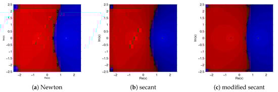
Figure 2. Dynamical planes for $f_1\left(z\right)=sin\left(z\right)-z^2+1$.

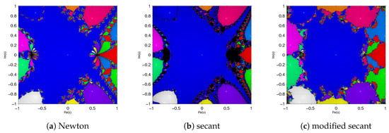
Figure 3. Dynamical planes for $f_2\left(z\right)=(z-1)(z^{10}+z^3+1)sin\left(z\right)$.

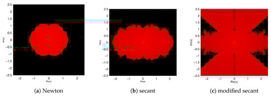
Figure 4. Dynamical planes for $f_3\left(z\right)=arctanz$.

In Table 2 the numerical results corresponding to the vectorial functions $F_4(x_1,x_2)$, $F_5(x_1,x_2)$ and $F_6(x_1,x_2,x_3)$ are presented. There is nothing significant in these results, they are those expected taking into account the theoretical results. In this case, the definition of ACOC is the same as before, replacing the absolute value by the norm. For systems $F_4\left(x\right)=0$ and $F_5\left(x\right)=0$, we show in Figure 5 and Figure 6 the basins of attraction of each root. In the first case, the three methods behave similarly, but in the second one, Newton’s scheme presents some black regions that do not appear in the modified secant method.

Table 2. Numerical results for the vectorial functions $F_4\left(x\right)$, $F_5\left(x\right)$, $F_6\left(x\right)$.

$F_4(x_1,x_2)=(x_1^2-1,x_2^2-1)$,     $x^{\left(0\right)}=(0.5,0.5)$,    $\xi =(1,1)$
Method	ACOC	Iter	$||x^{(k+1)}-x^{\left(k\right)}||$	$||F\left(x^{(k+1)}\right)||$
Newton	2.00	6	$1.5\times {10}^{-15}$	$1.7\times {10}^{-30}$
Secant	1.62	9	$1.3\times {10}^{-20}$	$6.9\times {10}^{-33}$
SecantM	1.88	7	$2.3\times {10}^{-17}$	$3.9\times {10}^{-33}$
$F_5(x_1,x_2)=(x_1^2-x_1-x_2^2-1,x_2-sin{x}_1)$,     $x^{\left(0\right)}=(1.5,1)$,     $\xi \approx (1.95,0.93)$
Method	ACOC	Iter	$||x^{(k+1)}-x^{\left(k\right)}||$	$||F\left(x^{(k+1)}\right)||$
Newton	2.02	6	$8.4\times {10}^{-18}$	$2.5\times {10}^{-35}$
Secant	1.62	8	$1.0\times {10}^{-16}$	$6.4\times {10}^{-27}$
SecantM	1.87	7	$2.5\times {10}^{-24}$	$7.65\times {10}^{-41}$
$F_6(x_1,x_2,x_3)=(x_1{x}_2-1,x_2{x}_3-1,x_1{x}_3-1)$,     $x^{\left(0\right)}=(0.5,0.5,0.5)$,     $\xi =(1,1,1)$
Method	ACOC	Iter	$||x^{(k+1)}-x^{\left(k\right)}||$	$||F\left(x^{(k+1)}\right)||$
Newton	2.00	6	$1.9\times {10}^{-15}$	$2.0\times {10}^{-30}$
Secant	1.62	9	$1.6\times {10}^{-20}$	$8.4\times {10}^{-33}$
SecantM	1.94	7	$2.8\times {10}^{-17}$	$1.5\times {10}^{-33}$

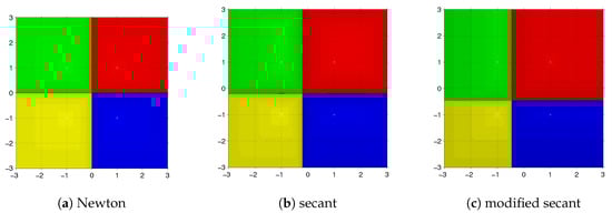
Figure 5. Dynamical planes for $F_4(x_1,x_2)=(x_1^2-1,x_2^2-1)$.

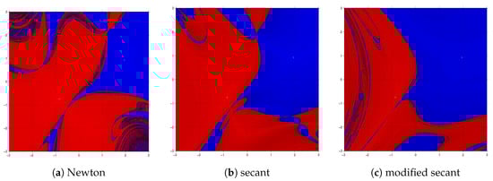
Figure 6. Dynamical planes for $F_5(x_1,x_2)=(x_1^2-x_1-x_2^2-1,x_2-sin{x}_1)$.

4. Conclusions

The technique of introducing accelerating parameters allows us to generate new methods with higher convergence order than the original one, with the same number of functional evaluations. The increase is more significant if we start from a method with high order of convergence. As far as we know, this is the first time that an iterative method with memory for solving nonlinear systems is designed by using Newton polynomial interpolation with several variables of second degree. In addition to obtaining the expression of what we called modified secant method, a dynamical study was carried out adapting tools from the dynamics of methods without memory to methods with memory. Although numerically computing the divided differences is hard, methods with memory show a very stable dynamical behavior, even more than other known methods without memory.

References

- Ortega, J.M.; Rheinboldt, W.C. Iterative Solutions of Nonlinear Equations in Several Variables; Academic Press: New York, NY, USA, 1970. [Google Scholar]
- Traub, J.F. Iterative Methods for the Solution of Equations; Chelsea Publishing Company: New York, NY, USA, 1982. [Google Scholar]
- Soleymani, F.; Lotfi, T.; Tavakoli, E.; Khaksar Haghani, F. Several iterative methods with memory using self-accelerators. Appl. Math. Comput. 2015, 254, 452–458. [Google Scholar] [CrossRef]
- Petković, M.S.; Neta, B.; Petković, L.D.; Džunić, J. Multipoint Methods for Solving Nonlinear Equations; Elsevier Academic Press: New York, NY, USA, 2013. [Google Scholar]
- Petković, M.S.; Sharma, J.R. On some efficient derivative-free iterative methods with memory for solving systems of nonlinear equations. Numer. Algorithms 2016, 71, 457–474. [Google Scholar] [CrossRef]
- Narang, M.; Bhatia, S.; Alshomrani, A.S.; Kanwar, V. General efficient class of Steffensen type methods with memory for solving systems of nonlinear equations. Comput. Appl. Math. 2019, 352, 23–39. [Google Scholar] [CrossRef]
- Potra, F.A. An error analysis for the secant method. Numer. Math. 1982, 38, 427–445. [Google Scholar] [CrossRef]
- Ostrowski, A.M. Solution of Equations and Systems of Equations; Academic Press: New York, NY, USA, 1960. [Google Scholar]
- Michelli, C.A. On a Numerically Efficient Method for Computing Multivariate B-Splines. In Multivariate Approximation Theory; Schempp, W., Zeller, K., Eds.; Birkhäuser: Basel, Switzerland, 1979; pp. 211–248. [Google Scholar]
- Potra, F.-A.; Ptak, V. Nondiscrete Induction and Iterative Processes; Pitman Publising INC: Boston, MA, USA, 1984. [Google Scholar]
- Fatou, P. Sur les équations fonctionelles. Bull. Soc. Math. Fr. 1919, 47, 161–271. [Google Scholar] [CrossRef]
- Julia, G. Mémoire sur l’iteration des fonctions rationnelles. J. Math. Pures Appl. 1918, 8, 47–245. [Google Scholar]
- Robinson, R.C. An Introduction to Dynamical Systems, Continous and Discrete; American Mathematical Society: Providence, RI, USA, 2012. [Google Scholar]
- Cordero, A.; Torregrosa, J.R. Variants of Newton’s method using fifth-order quadrature formulas. Appl. Math. Comput. 2007, 190, 686–698. [Google Scholar] [CrossRef]
- Campos, B.; Cordero, A.; Torregrosa, J.R.; Vindel, P. A multidimensional dynamical approach to iterative methods with memory. Appl. Math. Comput. 2015, 271, 701–715. [Google Scholar] [CrossRef]
- Chicharro, F.I.; Cordero, A.; Torregrosa, J.R. Drawing Dynamical Parameters Planes of Iterative Families and Methods. Sci. World J. 2013, 2013. [Google Scholar] [CrossRef] [PubMed]
© 2019 by the authors. Licensee MDPI, Basel, Switzerland. This article is an open access article distributed under the terms and conditions of the Creative Commons Attribution (CC BY) license (http://creativecommons.org/licenses/by/4.0/).