Abstract
Coupled fluid-structure is significant in many aspects of engineering applications such as aerospace fuel tanks, the seismic safety of storage tanks and tuned liquid dampers. Numerical investigation of the effects of thin plate cover over a cylindrical rigid fuel tank filled by an inviscid, irrotational, and incompressible fluid is investigated. Governing equations of fluid motion coupled by plate vibration are solved analytically. A parameter study on the natural frequency of coupled fluid-structure interaction is performed. The results show the non-dimensional natural frequency of coupled fluid-structure is a function of mass ratio, plate elasticity number and aspect ratio. This function is derived numerically for high aspect ratios which in companion with a semi-analytical could be used in the engineering design of liquid tanks with a cover plate.
1. Introduction
The coupling problem of structure and fluid interaction is a classic problem interested in various engineering applications such as vehicle dynamics, aircraft dynamics, and storage tanks [1,2,3,4,5]. The storage tanks usually built from strong materials such as steels (for drums), stainless steels, concrete, aluminum alloys, fiber-reinforced plastics (for fiber drum), and Timber which can bear large elastic vibrational energy. These tanks are exposed to dead and live loads such as snow, wind (vortex oscillation), seismic, buckling, and earth pressures. When the structure is assumed to have the many mass vibration system, modal analysis is a useful tool for the design of yield shear force of the convective mass vibration, damage to the structure (cumulative plastic strain energy), and water pressure imposed on the tank. That analysis needs the natural frequency of the maximum number of vibration modes that influence seismic responses.
One of the first analytical methods proposed to solve that problem is the Rayleigh–Ritz method [6]. The application of the method of Rayleigh–Ritz on the structure and fluid interaction with weak coupling [5] and strong coupling [7] was investigated by Amabili [7]. Various methods are applied to find the solution of the coupled fluid-structure interaction such as artificial spring method [8], finite element formulation [9], Galerkin method [10], time-marching technique [11], collocation method [12], Rayleigh quotients method [13], boundary elements method [14], boundary integral equation method [15]. Various numerical methods such as finite element, collocation, Rayleigh, boundary elements, and boundary integral method are the approximation to the exact solution. In the Rayleigh–Ritz method, the approximations to eigenvalue equations are found [5]. The finite element method analytical solution of boundary value problems is used to get a system of algebraic equations. In the Galerkin method [10] which is the popular method of finite element formulation [9], the differential equation is converted from a continuous operator problem to a discrete problem. In the collocation method, the idea is to choose a finite-dimensional space of proposed polynomial solutions and several domain points that satisfy the given equation at the collocation points [12]. In the boundary element method [14] the integral equations are solved by Green’s function elements connecting pairs of source and field patches defined by the mesh form a matrix. The boundary element method [15] is often more efficient than other methods [2] when there is a small surface to volume ratio. Conceptually, it works by constructing the surface mesh. However, for many problems boundary element methods are significantly less efficient than volume-discretization methods (finite element method, finite difference method, finite volume method). The added complexity of the boundary integral equation method could be overwhelmed by Compression techniques. Computational time and the storage requirements by boundary element formulations grow according to the square of the problem size while the finite element matrices are typically grown linearly with the problem size.
The fluid-structure coupling problem considered for various fluids such as dense fluids [16], the frictionless liquid in zero gravity [17], and compressible fluid [18], filled with non-viscous liquid [19] and various filling ratios for fluid-filled [19] and partially filled [20] were discussed in the literature. One of the most interesting geometries is a circular cylinder container. A drum (also called barrels in common usage) used in the shipping of dangerous powders and liquids, with 208 liters volume, has an 880 millimeters tall and 610 millimeters diameter (). Similar geometry is used for a barrel of crude oil (72 cm × 43 cm).
On the other hand, the types of solid structures connected with fluid were composed of cylindrical baffles [21], annular cylindrical tanks [22], ring-stiffeners and flexible bottom [23], annular baffle [24], vertical baffle [25], submerged components [26], internal bodies [27,28], two identical plates [29], immersed plate in a container [30]. As well the elastic structure bonding the fluids were initially bent cylindrical shells [31] and composite shells with orthogonal stiffeners [32]. Based on the size the containers are flexible and rigid. The design of a fluid-structure coupling problem in a cylindrical tank is an interesting research theme with possible engineering practical applications on stiffeners. Drums have chimes or rims at ends (chines). Most steel drums have reinforcing rolling hoops or rings of thickened metal or plastic. Amabili [23] investigated the effect of ring-stiffeners and flexible bottom on sloshing modes in cylindrical containers and drums.
Amabili [33] addresses a research theme in the area of fluid–solid interaction, focusing the analytical solution of an interesting problem of coupled vibration of a fluid-filled cylindrical rigid tank with an elastic top cover. The two kinds of drums are barrels (welded top) and the open top. Vibrations of a circular flexible membrane or elastic plates resting on a sloshing liquid is a class of problem which first studied by Amabili [33], for annular plate cover by Kim and Lee [34] and fully covered case by Bauer [35]. Bauer [35] makes use of the Fourier–Bessel series expansion to analytically derive the solution of the addressed problem, and perform a parametric study on the natural frequency of the coupled fluid-structure interaction in clamped boundary condition and for varying characteristic values of the system.
Considering all of the above, there is no research performed on the analytical solution of rigid tank coupling with elastic cover with different support conditions. The analytical solution is not easy to use by engineers but is the exact solution of the problem and has the benefits of a minimum number of parameters and accuracy over the other methods such as finite element, collocation, Rayleigh, boundary elements, and boundary integral method. The aim of the current study is finding the analytical solution of a fluid-filled cylindrical container with rigid sides and bottom and elastic circular plate over the top surface. In the next section mathematical model of the system in the fluid and solid parts is presented.
2. Mathematical Model
2.1. Fluid Model
The schematic of the problem is shown in Figure 1. If the fluid field equations are linearized for small displacements based on the linearized theory of water the flow potential is found from the Laplace equation. By assuming a simple harmonic motion with a radian frequency , the velocity potential is
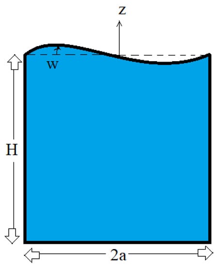
Figure 1.
Geometry of the problem.
In order to calculate the flow potential distribution, , in the above equation (i.e., Equation (1)) based on a typical power series, the fluid domain is defined mathematically as
The modal expansion method could be used for the fluid velocity potential as
where is time-independent velocity potentials, the is time-dependent coefficient of n-th mode, and is n-th sloshing position dependent eigenfunctions.
The governing equation in the fluid region for is
which satisfies the following boundary conditions:
on the symmetric line (for ),
on the rigid wall (for ), and
on the container bottom (for ). The three–dimensional view of the problem with fluid–solid interaction surface and the side boundary condition is shown in Figure 2. The solution of above equations are (see Equation (1.40) in [1])
where and are time–dependent coefficients could be found from the initial conditions of free–surface or pressure distribution, is mode coefficient in fluid domain, is order m of first kind Bessel function. The above definition should satisfy the linearized (neglecting from circumferential and radial displacement) fluid–surface Kinematic boundary condition coupled by solid
for where in the case of fluid without a cover the eigenvalue of the system is found from the linearized boundary condition at free-surface
for in which, g denotes the gravitational acceleration. The use of the analytical solution in the above equation leads to (see Equation (1.43a) in [1])
where is the frequency of mode in fluid domain. As well for the sake of simplicity, the axi-symmetric modes just considered then the solution in the fluid domain is
and by assuming the axi-symmetric modes and wall boundary condition at the outer wall (See Equation (6)) then in the fluid domain, the solution is
the roots of Equation (13) are presented in Table 1.
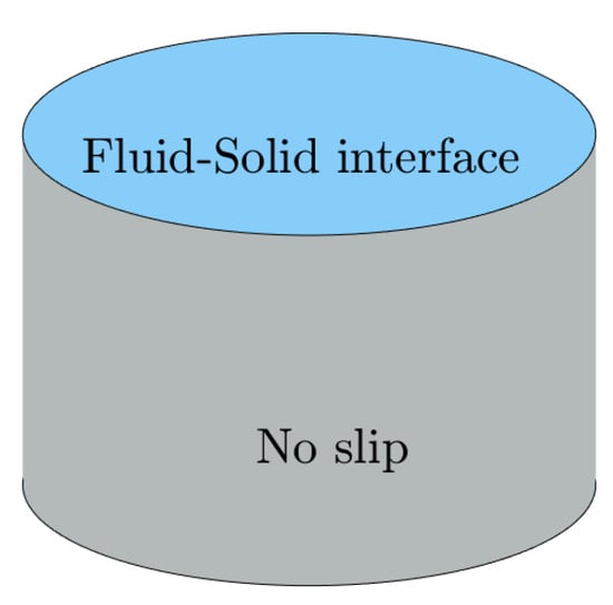
Figure 2.
The 3D view of the tank with boundary condition.

Table 1.
Values of satisfy Equation (13).
2.2. Solid Model
The governing equation of the solid motion with the variable of w for the transverse displacement of a bent thin plate is presented by the following partial differential equation
where the flexural rigidity (D) is defined by
and is the biharmonic operator that can be expanded as follows
where
As the pressure could be presented in the form of a harmonic function in time
and displacement could be presented in the form of a harmonic function in time
the classical differential equation of solid displacement from Equations (14) can be rewritten as
The pressure is made of two components of fluid pressure, , and the pressure caused by surface elevation, ,
As the fluid is considered to be stuck to the solid at to boundary, the surface elevation pressure is found by [35]
Using Bernoulli equation for the fluid pressure, , and neglecting the nonlinear terms, the pressure of the fluid could be related to the time derivative of velocity potential of the fluid () and fluid density () [33]
3. Analytic Solution Procedure
3.1. Analytic Solution of Solid Deflection with Fluid Load
The general idea, for the solution of an inhomogeneous linear PDE with Equation (24) is to split its solution into two parts
The first term, , is the homogeneous solution of Equation (24) and next term, , is the in-homogeneous solution of the Equation (24) which has the same boundary condition (plus the initial conditions as the time is a variable) of the full problem.
For the solution of the homogeneous equation, one can assume the Fourier components in as,
where
and
respectively, where and are the second and first kind Bessel functions, respectively. As well, the , and , are second and first kind modified Bessel functions. The mode coefficients () determine the significance of the mode shape and could be found from the initial condition and the boundary conditions. Thus, the general solution of a solid governing equation in polar coordinates is (See Equation (1.18) in [5])
When the polar coordinate origin is considered the same as the circular plate center (without internal hole), the terms of Equation (1.18) in [5] involving and neglected as the value of the deflection at singular point () has a finite value. When these simplifications are employed, the modal displacement will be reduced to the following equation for a typical mode
3.2. Boundary Conditions
3.2.1. Clamped Plate
The boundary condition of zero deflection at the perimeter is used both for clamped plate and simply supported case. For the simply supported case and clamped plate, the plate displacement is zero on the perimeter of the plate (),
Since the boundary condition of Equation (35) for constant terms (i.e., n = 0) leads to
and for each cosine term (i.e., where ) leads to
The second boundary condition which is devoted to just clamped plate case is
The first derivative of deflection with respect to the r at is
3.2.2. Simply Supported Plate
Simply supported plate is a combination of zero deflection at perimeter (i.e., Equations (38) and (39)) and zero radial twisting moment at perimeter. As well the radial twisting moment
where at plate edge must be zero. i.e.,
The first deriviate of deflection respect to the r at is retrieved from Equation (41) and the second deriviate of deflection respect to the r at is
The second derivative of deflection with respect to at is
Since
The boundary condition of Equation (45) for constant terms (i.e., n = 0) leads to
or in a simplified way
and for each cosine term (i.e., where ) leads to
rearranged in the form
3.2.3. Kinematic Boundary Condition at Free Surface
Finally by considering the Kinematic boundary condition (See Equation (9)) of the fluid–solid interaction for the region of the top surface of the fluid under the circular plate with the time dependency relations (See Equations (1) and (19))
for all values of on the plate position which is simplified by the aid of Equations (1) and (19) to
The equation (Equation (54)) can be explained by the system of equations with fluid motion modes expansion.
The boundary condition at top surface (Equation (54))
The boundary condition of Equation (54) for constant terms (i.e., n = 0) leads to
and for each cosine term (i.e., where ) leads to
Multiplying the above equation (Equation (56)) by and integrating over the whole plate domain (i.e., ) for to the system of equations are closed.
4. Numerical Implementation
If the finite numbers of series is considered (i.e., and ), for variables (i.e., 1 for , M + 1 for , and M for , and MN for ) there are equations for simply supported case (i.e., 1 in Equation (38), M + 1 in Equation (39), 1 in Equation (50), M + 1 in Equation (52), and in multiplying Equation (56) by Bessel functions) and there are equations for clamped case (i.e., 1 in Equation (38), M + 1 in Equation (42), 1 in Equation (43), M + 1 in Equation (52), and in multiplying Equation (56) by Bessel functions). The Appendix A formula is used to simplify the final formulas. The equations and variables are summarized in Table 2 and in detail in Table 3 and Table 4.
Table 2.
System of equations and variables.
Table 3.
Matrix of equations and variables for simply supported case.
Table 4.
Matrix of equations and variables for clamped case.
If the variables seen in a matrix form
where and .
The equations can be re-written in the form matrix as
4.1. Simply Supported Plate
In simply supported case, the rows of A are derived from Equations (38), (48), and (56) respectively.
The coefficient matrix would be obtained as
where
- is a matrix as
- is a matrix aswhere m is from 1 to M.
- is a matrix as
- is a matrix as
- is a matrix aswhere m is from 1 to M.
- is a matrix as
- is a matrix as
- is a matrix aswere l is from 0 to M and in calculation of instead of the uniform unit function () should be considered.i.e.,
- is a matrix aswhere k is from 0 to M and m is from 1 to M. As well in calculation of at k =0instead of the uniform unit function () should be considered.
- is a matrix aswhere k is from 0 to M. In calculation of atk =0 instead of the uniform unit function () should be considered.
- is a matrix aswhere k is from 0 to M. At k = 0 instead of the uniform unit function () is considered in calculation of .
- is a diagonal matrix where the element of (n is from 1 to N) where defined as
- is a diagonal matrix where the element of (n is from 1 toN) which defined as
- is a matrix asn is from 1 to N and mis from 1 toM.
- is a diagonal matrix where the element of (n is from 1 to N) where defined as
- is a diagonal matrix where the element of (n is from 1 to N) which defined as
- is a diagonal matrix where the element of (n is from 1 to N) wheredefined as
- is a matrix which element of is found fromwhere , , and p(i,j) = (j − 1)N + i.
- is a matrix as which element of is found fromwhere , , , and p(i,j) = (j −1)N + i.
- is a matrix as where element of is found fromwhere , , m is from 1 to M, j is from 1 toM, p(i,j) = (j − 1)N + i, and q(n,m) = (m − 1)N + n.
4.2. Clamped Plate
The matrix A is defined by
The coefficient matrix would be obtained as
The coefficients of A in above equation (Equation (86)) are same as simply supported case except:
- is a matrix as
- is a matrix as
- is a diagonal matrix where the element of (n is from 1 to N) are defined as
- is a diagonal matrix where the element of (n is from 1 toN) which defined as
5. Results and Discussion
The analytical solutions which are obtained in the previous section, are investigated numerically for the practical case. The numerical results in the current section have been derived by developing code inside the MATLAB software. The natural frequencies are presented in unit where . Usual material properties of the water tank storage are given in Table 5. The values are not fixed and are averaged from various references. For example, the stone Poisson ratio is reported between 0.2 and 0.3 in various references but the value of 0.25 is chosen for the table. The last two rows of the Table 5 calculated for the special case of h = 1 mm and a = 1 m. As shown for that values the first parameter is in order of and second parameter is in order of . The geometrical and physical properties of the fluid material and solid material are presented in Table 6. Relative errors of computing axi-symmetric modes of the clamped cover plates are presented in Table 7. Table 7 presents the relative error () versus mode number and aspect ratios where the solution with ten expansion terms is considered as the exact frequency (M = 10). The performance of the method is comparable with the Table 4 in Amabili [33] where the convergence of the solution was discussed. As shown the use of the current method causes the precise results in most cases by three terms in fluid expansion series with three terms. Table 4 in Amabili [33] used 10 terms for the solid motion (in Table 7 just one term is used for solid deflection) and 50 terms for liquid potential (As seen in Table 7 the M = 3 matches the exact solution). Assessment of the non-dimensional angular velocity () versus height ratio of the tank () for the boundary condition of the clamped solid at the three axi-symmetric modes with minimum values ( and ) against the values presented in Tables 1 and 2 of Amabili [33] are presented in Table 8. As shown a good agreement seen among the current study results and those of Bauer ([35]) and Amabili ([33]) for axi-symmetric modes of the clamped cover plates (for and modes). Results were found by one-term expansion of the solid plate deflection and 4 terms for the liquid potential.
Table 5.
Usual material properties of the water tank storage.
Table 6.
Geometric and material properties of the system.
Table 7.
Relative errors of computing axi-symmetric modes of the clamped cover plates.
Table 8.
Comparison of the first three axi-symmetric modes of the clamped cover plates with Amabili [33].
The non-dimensional fluid-structure frequencies for simply supported boundary condition (presented by the dashed line in Figure 3) and clamped boundary condition (presented by solid line in Figure 3) at , , and axi-symmetric mode is plotted in Figure 3. As shown, the agreement of results of the current study with non-dimensional fluid-structure frequencies for clamped plate obtained by Bauer ([35]) is perfect. As exposed in all cases the clamped boundary condition caused higher frequencies than the simply supported plate.
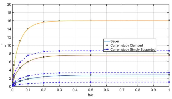
Figure 3.
The non-dimensional fluid-structure frequencies for simply supported boundary condition (dashed lines) and clamped boundary condition (solid lines) at , , and axi-symmetric mode .
5.1. Clamped Plate
Assessment of the present results and the Bauer ([35]) results for other figures in plate cover case has been performed in Figure 4. The dominant modes of the structure i.e., the first three mode shapes are illustrated in Figure 4. The non-dimensional fluid-structure frequencies for clamped plate , , and axi-symmetric mode , , , and axi-symmetric mode , , , and axi-symmetric mode , , , and axi-symmetric mode is plotted in Figure 4. As shown, the agreement of results of the current study with non-dimensional fluid-structure frequencies for clamped plate obtained by Bauer ([35]) are matching. As for the common storage tank the aspect ratio () is above the unity the parameter study of the natural frequencies as the function of the elastic parameter () and mass ratio () is useful for engineering design. For the first mode natural frequency at high aspect ratios, the natural frequency grows monotonically with . As shown by the increase of the elastic parameter () and the mass ratio () the non-dimensional circular frequency () is increased. The sensitivity analysis of the results show that the mass ratio () is the most important parameter on the detect of natural frequency. The non-dimensional fluid-structure frequencies for clamped plate versus and axi-symmetric mode for various is plotted in Figure 5. As shown by the increase of the elastic parameter () and mass ratio () is useful for engineering design. As shown by the increase of elastic parameter () and mass ratio () the non-dimensional circular frequency () is increased. The non-dimensional fluid-structure frequencies for clamped plate versus and axi-symmetric mode for various is plotted in Figure 6. As illustrated by an increase of the elastic parameter () and mass ratio () is useful for engineering design. As shown by the increase of elastic parameter () and mass ratio () the non-dimensional circular frequency () is increased. The non-dimensional fluid-structure frequencies for clamped plate versus and axi-symmetric mode for various is plotted in Figure 7. As illustrated by an increase of the elastic parameter () and mass ratio () is useful for engineering design. As shown by the increase of elastic parameter () and mass ratio () the non-dimensional circular frequency () is increased.
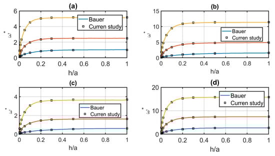
Figure 4.
The non-dimensional fluid-structure frequencies for clamped plate (a) , , and axi-symmetric mode (b) , , and axi-symmetric mode (c) , , and axi-symmetric mode (d) , , and axi-symmetric mode .
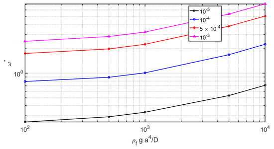
Figure 5.
The non-dimensional fluid-structure frequencies for clamped plate versus and axi-symmetric mode for various .
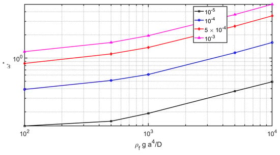
Figure 6.
The non-dimensional fluid-structure frequencies for clamped plate versus and axi-symmetric mode for various .
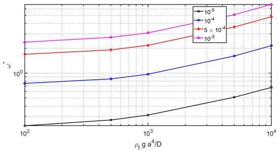
Figure 7.
The non-dimensional fluid-structure frequencies for clamped plate versus and axi-symmetric mode for various .
5.2. Simply Supported Plate
The modal analysis is required to find the inherent dynamic properties of the any domain in terms of its natural frequencies. The non-dimensional fluid-structure frequencies for simply supported plate , , and axi-symmetric mode , , , and axi-symmetric mode , , , and axi-symmetric mode , , , and axi-symmetric mode is plotted in Figure 8. The dominant modes of the structure i.e., the first three mode shapes are illustrated in Figure 8. As illustrated in Figure 8, the natural frequencies are increased by an increase of aspect ratio. The comparison of the Figure 8 and Figure 4 is not simple such as the results of zero modes Figure 3 for clamped plate and simply supported case. As exposed in some cases the clamped boundary condition caused higher frequencies than the simply supported plate and in some cases it was vice versa.
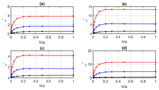
Figure 8.
The non-dimensional fluid-structure frequencies for simply supported plate (a) , , and axi-symmetric mode (b) , , and axi-symmetric mode (c) , , and axi-symmetric mode (d) , , and axi-symmetric mode .
The non-dimensional fluid-structure frequencies for clamped plate versus and axi-symmetric mode for various is plotted in Figure 9. As shown the parameter study of the natural frequencies as the function of the elastic parameter () and mass ratio () presents a linear relation between the parameters in comparison with the nonlinear case was shown for clamped case in Figure 5. As shown by the increase of elastic parameter () and mass ratio () the non-dimensional circular frequency () is increased. The sensitivity analysis of the results show that even the mass ratio () is the most important parameter on the detect of natural frequency, the elastic parameter () is more important than the nonlinear case was shown for clamped case in Figure 5. The non-dimensional fluid-structure frequencies for clamped plate versus and axi-symmetric mode () for various is plotted in Figure 10. In this case in contract with linear behavior of the clamped case in Figure 5 a parabola shape is seen. It means that there are some optimal values of elastic parameter () where the natural angular velocity of the axi-symmetric mode () is minimized. This frequency is important in horizontal movement of the sloshing tanks. The non-dimensional fluid-structure frequencies for clamped plate versus and axi-symmetric mode for various is plotted in Figure 11. The fundamental angular velocity of the axi-symmetric mode () shows a parabola shape same as the fundamental angular velocity of the axi-symmetric mode ().
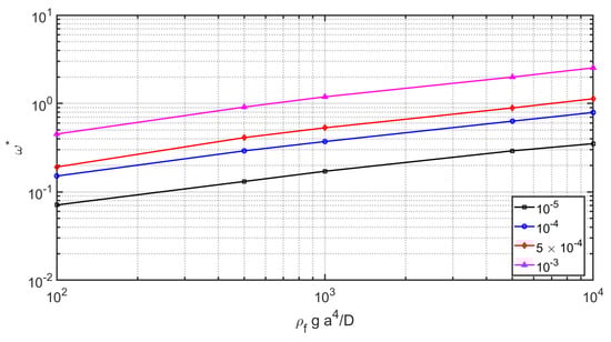
Figure 9.
The non-dimensional fluid-structure frequencies for simply supported plate versus and axi-symmetric mode for various .
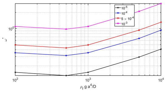
Figure 10.
The non-dimensional fluid-structure frequencies for simply supported plate versus and axi-symmetric mode for various .
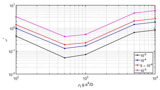
Figure 11.
The non-dimensional fluid-structure frequencies for simply supported plate versus and axi-symmetric mode for various .
6. Conclusions
The analytical investigation of the effects of thin plate cover over a cylindrical rigid fuel tank filled by an inviscid, irrotational, and incompressible fluid was investigated in the current study. Governing equations of fluid motion coupled by plate vibration are found by the application of the Fourier–Bessel series expansion. A parameter study on the fundamental angular velocity of coupled fluid-structure motion is performed. The results show the non-dimensional fundamental angular velocity of a coupled fluid-structure system is a function of mass ratio, plate elasticity number and aspect ratio. This function is derived numerically for high aspect ratios which in companion with a semi-analytical could be used in the engineering design of liquid tanks with a cover plate. As illustrated by an increase of the elastic parameter () and mass ratio () is useful for engineering design. As shown by the increase of elastic parameter () and mass ratio () the non-dimensional circular frequency () is increased. As well the sensitivity analysis of the results shows that the mass ratio () is the most important parameter on the detect of natural frequency.
Funding
This research received no external funding.
Conflicts of Interest
The author declare no conflict of interest.
Appendix A
The following formulas were used in simplification of Equations
References
- Ibrahim, R.A. Liquid Sloshing Dynamics; Cambridge University Press: Cambridge, UK, 2005. [Google Scholar]
- Miles, J.W. On the sloshing of liquid in a flexible tank. J. Appl. Mech. E 1958, 25, 277–283. [Google Scholar]
- Morand, H.J.P.; Ohayon, R. Fluid-structure Interaction. Applied Numerical Methods; Wiley: New York, NY, USA, 1995. [Google Scholar]
- Yamaki, N.; Tani, J.; Yamaji, T. Free vibration of a clamped-clamped circular cylindrical shell partially filled with fluid. J. Sound Vib. 1984, 94, 531–550. [Google Scholar]
- Leissa, A.W. Vibration of Plates; NASA SP-1960; NASA: Washington, DC, USA, 1969.
- Zhu, F. Rayleigh-Ritz method in coupled fluid-structure interacting systems and its applications. J. Sound Vib. 1995, 186, 543–550. [Google Scholar] [CrossRef]
- Amabili, M. Ritz method and substructuring in the study of vibration with strong fluid-structure interaction. J. Fluids Struct. 1997, 11, 507–523. [Google Scholar] [CrossRef]
- Amabili, M. Shell-plate interaction in the free vibrations of circular cylindrical tanks partially filled with a liquid: The artificial spring method. J. Sound Vib. 1997, 199, 431–452. [Google Scholar] [CrossRef]
- Mazuch, T.; Horaek, J.; Trnka, J.; Vesely, J. Natural modes and frequencies of a thin clamped- free steel cylindrical storage tank partially filled with water: FEM and measurements. J. Sound Vib. 1996, 193, 669–690. [Google Scholar] [CrossRef]
- Cheung, Y.K.; Zhou, D. Hydroelastic vibration of a circular container bottom plate using the Galerkin method. J. Fluids Struct. 2002, 16, 561–580. [Google Scholar] [CrossRef]
- Jadic, I.; So, R.M.C.; Mignolet, M.P. Analysis of fluid-structure interactions using a time-merching technique. J. Fluids Struct. 1998, 12, 631–654. [Google Scholar] [CrossRef]
- Mikami, T.; Yoshimura, J. The collocation method for analyzing free vibration of shells of revolution with either internal or external fluids. Comput. Struct. 1992, 44, 343–351. [Google Scholar] [CrossRef]
- Zhu, F. Rayleigh quotients for coupled free vibrations. J. Sound Vib. 1994, 171, 641–649. [Google Scholar] [CrossRef]
- Hatzigeorgiou, G.D.; Beskos, D.E. Dynamic inelastic structural analysis by the BEM: A review. Eng. Anal. Bound. Elem. 2011, 35, 159–169. [Google Scholar] [CrossRef]
- Ergin, A.; Ugurlu, B. Hydroelastic analysis of fluid storage tanks by using a boundary integral equation method. J. Sound Vib. 2004, 275, 489–513. [Google Scholar] [CrossRef]
- Amabili, M. Vibrations of circular tubes and shells filled and partially immersed in dense fluids. J. Sound Vib. 1999, 221, 567–585. [Google Scholar] [CrossRef]
- Bauer, H.F.; Komatsu, K. Coupled frequencies of a hydroelastic system of an elastic two-dimensional sector-shell and frictionless liquid in zero gravity. J. Fluids Struct. 1994, 8, 817–831. [Google Scholar] [CrossRef]
- Jeong, K.H. Hydroelastic vibration of two annular plates coupled with a bounded compressible fluid. J. Fluids Struct. 2006, 22, 1079–1096. [Google Scholar] [CrossRef]
- Amabili, M. Vibrations of fluid-filled hermetic cans. J. Fluids Struct. 2000, 14, 235–255. [Google Scholar] [CrossRef]
- Ergin, A.; Temarel, P. Free vibration of a partially fluid-filled and submerged horizontal cylindrical shell. J. Sound Vib. 2002, 254, 951–965. [Google Scholar] [CrossRef]
- Maleki, A.; Ziyaeifar, M. Sloshing damping in cylindrical liquid storage tanks with baffles. J. Sound Vib. 2008, 311, 372–385. [Google Scholar] [CrossRef]
- Amabili, M.; Dalpiaz, G. Vibrations of base plates in annular cylindrical tanks: Theory and experiments. J. Sound Vib. 1998, 210, 329–350. [Google Scholar] [CrossRef]
- Amabili, M.; Paidoussis, M.P.; Lakis, A.A. Vibrations of partially filled cylindrical tanks with ring-stiffeners and flexible bottom. J. Sound Vib. 1998, 213, 259–299. [Google Scholar] [CrossRef]
- Gavrilyuk, I.; Lukovsky, I.; Trotsenko, Y.; Timokha, A. Sloshing in a vertical circular cylindrical tank with an annular baffle. Part 1. Linear fundamental solutions. J. Eng. Math. 2006, 54, 71–88. [Google Scholar] [CrossRef]
- Evans, D.V.; McIver, P. Resonant frequencies in a container with a vertical baffle. J. Fluid Mech. 1987, 175, 295–307. [Google Scholar] [CrossRef]
- Mitra, S.; Sinhamahapatra, K.P. Slosh dynamics of liquid–filled containers with submerged components using pressure-based finite element method. J. Sound Vib. 2007, 304, 361–381. [Google Scholar] [CrossRef]
- Watson, E.B.B.; Evans, D.V. Resonant frequencies of a fluid in containers with internal bodies. J. Eng. Math. 1991, 25, 115–135. [Google Scholar] [CrossRef]
- Jeong, K.H.; Kang, H.S. Free vibration of multiple rectangular plates coupled with a liquid. Int. J. Mech. Sci. 2013, 74, 161–172. [Google Scholar] [CrossRef]
- Jeong, K.H. Free vibration of two identical circular plates coupled with bounded fluid. J. Sound Vib. 2003, 260, 653–670. [Google Scholar] [CrossRef]
- Askari, E.; Jeong, K.H.; Amabili, M. Hydroelastic vibration of circular plates immersed in a liquid-filled container with free surface. J. Sound Vib. 2013, 332, 3064–3085. [Google Scholar] [CrossRef]
- Kovalichuk, P.S.; Fillin, V.G. On modes of flexural vibrations of initially bent cylindrical shells partially filled with a liquid. Int. Appl. Mech. 2003, 39, 464–471. [Google Scholar] [CrossRef]
- Lee, Y.S.; Kim, Y.W. Effect of boundary conditions on natural frequencies for rotating composite cylindrical shells with orthogonal stiffeners. Adv. Eng. Softw. 1999, 30, 649–655. [Google Scholar] [CrossRef]
- Amabili, M. Vibrations of circular plates resting on a sloshing liquid: Solution of the fully coupled problem. J. Sound Vib. 2001, 245, 261–283. [Google Scholar] [CrossRef]
- Kim, Y.W.; Lee, Y.S. Coupled vibration analysis of liquid-filled rigid cylindrical storage tank with an annular plate cover. J. Sound Vib. 2005, 279, 217–235. [Google Scholar] [CrossRef]
- Bauer, H.F. Coupled frequencies of a liquid in a circular cylindrical container with elastic liquid surface cover. J. Sound Vib. 1995, 180, 689–704. [Google Scholar] [CrossRef]
© 2019 by the author. Licensee MDPI, Basel, Switzerland. This article is an open access article distributed under the terms and conditions of the Creative Commons Attribution (CC BY) license (http://creativecommons.org/licenses/by/4.0/).