Resilient Collaborative Control Method for Transportation Hubs Considering Communication Reliability

Abstract

As traffic demand increases and intelligent transportation systems continue to develop, traffic signal control must operate reliably in complex and heterogeneous network environments, especially under communication instability. Traditional approaches often lack sufficient resilience when facing packet loss, delay, and other communication disturbances. This study proposes a resilient collaborative control (RCC) method for transportation hubs that explicitly considers communication reliability. A multi-layer computational framework is developed to support real-time mapping and interaction between physical and virtual networks. A fuzzy-logic-based communication state perception model is introduced to guide adaptive control-mode switching. To improve network-level performance, a recovery-oriented optimization algorithm is applied for dynamic load balancing across the hub area. Co-simulation results show that, compared with traditional adaptive control, the proposed method reduces average vehicle delay by 42.3%, increases network speed by 52.3%, shortens recovery time by 63%, and improves the resilience index to 0.87. These results support the effectiveness of the proposed framework within the evaluated co-simulation setting.

1. Introduction

Modern traffic management has evolved into a complex network optimization problem. While intelligent transportation systems (ITSs) rely on seamless data exchange, real-world network environments often suffer from communication instability, such as packet loss and delays [1,2]. These disturbances threaten the reliability of traffic control, especially in large-scale hubs [3,4]. Traditional strategies, assuming ideal communication [5], frequently fail to maintain stability under uncertain network states. Without sufficient resilience, conditions like communication interruptions can lead to system paralysis [6]. Thus, developing computational methods to enhance the resilience of traffic networks is now a critical demand.

The integration of 5G and artificial intelligence has transitioned ITSs into a stage of networked intelligence [7,8], where signal control evolves through mathematical modeling and collaborative optimization [9,10]. However, this connectivity introduces a heavy dependence on communication infrastructure. In practice, network-induced disturbances can hinder accurate signal execution, leading to deteriorated performance in systems requiring dynamic load balancing. Addressing the coupling between communication reliability and control efficacy has therefore become a core challenge in network optimization.

Current research on traffic signal optimization primarily employs advanced computational technologies such as digital twins (DTs), deep reinforcement learning, and graph-based modeling. Adarbah et al. [11] proposed a DT-based management system using the BIRCH algorithm to optimize large-scale data processing, while Zhu et al. [12] developed a DT-enhanced adaptive framework to improve multi-intersection coordination. Kumarasamy et al. [13] further integrated DTs with multi-agent reinforcement learning to enhance system adaptability in dynamic environments. Nevertheless, current research still faces several limitations. Most studies assume fully stable and reliable networks, ignoring degradation phenomena such as delay and packet loss that frequently occur in practice [14]. Existing approaches often lack real-time perception and adaptive adjustment mechanisms for dynamic communication states [15]. Moreover, there is no systematic resilience evaluation framework; current research focuses primarily on normal operations without quantitatively assessing anti-interference and recovery capabilities under disturbances [16]. Few works have proposed effective emergency strategies for severe communication failures, with most systems reverting to fixed-time control and suffering significant performance loss [17]. Therefore, enhancing the robustness and recovery capability of traffic networks under abnormal communication conditions has become a critical challenge in network optimization.

To address these vulnerabilities, resilience theory offers a transformative perspective by emphasizing a system’s capacity to maintain core functions and recover rapidly from disturbances [18]. Integrating resilience into traffic control requires innovations in computational architectures and adaptive algorithms. As a bridge between physical and digital domains, DT technology provides the essential technical support for this integration by enabling real-time monitoring and virtual validation of control strategies [19]. Consequently, this study develops a communication-aware RCC framework tailored for large-scale transportation hubs. By combining resilience mechanisms with a multi-layer DT architecture, this research aims to enhance system trustworthiness and efficiency under unstable network conditions, providing both theoretical and practical guidance for network optimization in complex urban environments [20]. The main contributions of this paper are as follows:

• This paper proposes a communication-aware resilient collaborative control (RCC) framework for traffic signals in large-scale transportation hubs. By integrating traffic flow, communication network, and coupling models within a four-layer digital twin architecture, the framework enables real-time mapping and bidirectional interaction between the physical and virtual environments.
• This paper establishes a three-level resilience evaluation index system comprising performance, structural, and functional resilience and develops a fuzzy-logic-based communication state perception mechanism combined with time-series fault prediction. In particular, the proposed CQI-driven perception module explicitly links communication reliability (delay/loss/jitter) with control decision making and early warning.
• This paper designs an adaptive control strategy driven by communication quality indicators, enabling dynamic switching of control modes and parameters under varying network conditions. In addition, a DT-supported recovery mechanism with case library-assisted genetic algorithm initialization is introduced to accelerate restoration during interruption–recovery processes.
• SUMO–NS3 co-simulation results show that the proposed framework reduces vehicle delay, increases network speed, shortens recovery time, and improves the resilience index under communication-degraded conditions, compared with the adaptive control baselines considered in this study.

The remainder of this paper is organized as follows. Section 2 reviews related work. Section 3 introduces the construction of the communication-aware digital twin system. Section 4 presents the proposed RCC algorithm. Section 5 describes system implementation and simulation verification. Section 6 discusses computational overhead, scalability, and current limitations of the proposed framework. Finally, Section 7 concludes this paper.

2. Related Work

Traffic signal control has transitioned from localized adaptive methods to regional collaborative optimization. Digital twin (DT) technology has emerged as a cornerstone of this evolution, providing high-fidelity virtual–physical mapping for infrastructure lifecycle management [21] and network-level coordination [22]. Recent studies have demonstrated the efficacy of DTs in diverse applications, from railway level-crossing automation [23] to cluster-based traffic management [11], establishing a robust technical foundation for data-driven signal coordination.

Despite these advancements, existing collaborative frameworks often assume ideal network conditions, neglecting communication-induced degradations such as latency and packet loss [24]. Recent studies have shown that communication delays can significantly affect the operational performance of autonomous intersection management systems [25]. Conventional systems lack the necessary resilience to sustain performance during equipment failures or incidents [26,27]. Furthermore, the inability of current architectures to sense communication quality in real time hinders adaptive policy adjustment, necessitating a shift toward communication-aware control strategies [28].

To bridge this gap, we integrate resilience theory with DT technology to create a self-healing control environment. DTs provide the computational infrastructure for multi-source data fusion and virtual strategy verification [19,29], while resilience principles ensure the system maintains core functions and recovers rapidly from disturbances [30,31]. By incorporating distributed frameworks and intelligent recovery optimization [32], this integrated approach enables stable traffic service levels even within highly unstable communication environments.

3. Construction of Communication Perception Digital Twin System

To support resilient control in complex transportation hubs, a communication-aware DT system is constructed based on a four-level hierarchical architecture that facilitates a closed-loop flow from data perception to decision optimization. This hierarchical structure ensures that the virtual model accurately reflects physical dynamics while providing the computational foundation for resilient, intelligent control policies.

3.1. Integrated Modeling of Transportation and Communication

The integration of transportation and communication requires a bidirectional coupling mechanism, utilizing a cellular automata model to provide efficient, high-fidelity micro-traffic simulations for digital twin systems. By discretizing roads into cells and applying fundamental motion rules, this model reproduces complex traffic phases to enable real-time evaluation of signal control strategies. The motion state of the vehicle at time t is described by positions $x\left(t\right)$ and $v\left(t\right)$, and the updates at each time step follow the following rules.

(1) Acceleration rules: $v_n\left(t+1\right)=min\left(v_n\left(t\right)+1,v_{max}\right)$.

(2) Deceleration rules: $v_n\left(t+1\right)=min\left(v_n\left(t+1\right),d_n\left(t\right)\right)$.

$d_n\left(t\right)$ is the distance gap between vehicle n and the preceding vehicle. $d_n\left(t\right)=x_{n-1}\left(t\right)-x_n\left(t\right)-l_{veh}$.

(3) Random slowing down rule: $v_n\left(t+1\right)=max\left(v_n\left(t+1\right)-1,0\right)p_{slow}$.

(4) Location update: $x_n\left(t+1\right)=x_n\left(t\right)+v_n\left(t+1\right)$.

Here, $v_{max}$ is the maximum speed, $l_{veh}$ is the vehicle length, and $p_{slow}$ is the random slowing probability. Table 1 summarizes key parameters for both transportation and communication systems, such as speed limits and packet arrival rates, to provide the basis for coupling analysis.

Table 1. Key parameters of transportation communication fusion model.

Parameter Name	Symbol	Value Range	Unit	Description
Maximum Vehicle Speed	$v_{max}$	60–80	km/h	Maximum vehicle speed
Minimum Safe Distance	$d_{\mathrm{safe}}$	2–5	m	Minimum safe distance
Random Deceleration Probability	$p_{\mathrm{slow}}$	0.1–0.3	–	Random deceleration probability
Data Packet Arrival Rate	$\lambda$	50–200	packets/s	Data packet arrival rate
Average Service Time	$T_s$	5–20	ms	Average service time
Channel Bandwidth	$\mathrm{BW}$	10–100	Mbps	Channel bandwidth
Communication Delay Threshold	$D_{\mathrm{th}}$	100	ms	Communication delay threshold
Packet Loss Rate Threshold	$L_{\mathrm{th}}$	$<5$	%	Packet loss rate threshold

The transportation–communication coupling model establishes the interaction mechanism between the traffic subsystem and the communication subsystem. On the one hand, traffic states affect the offered load of the communication network: when the intersection flow increases, the number of V2I message exchanges between vehicle terminals and roadside units increases, which may cause channel congestion and increased transmission delay. We model this effect using a linear coupling function:

$$\mathcal{L}\left(t\right)=\alpha Q\left(t\right)+\beta V\left(t\right)+\gamma$$

(1)

where $Q\left(t\right)$ is the intersection traffic flow at time t, $V\left(t\right)$ is the number of onboard terminals connected to the communication network, and $\mathcal{L}\left(t\right)$ denotes the communication offered-load indicator derived from the NS-3 side (e.g., aggregated packet/request intensity within the same time interval). To make the parameter setting reproducible and evidence-based, $\alpha ,\beta ,\gamma$ are identified using the SUMO–NS-3 co-simulation data generated by the joint platform described in Section 5. Specifically, after removing the warm-up period, we construct a calibration dataset from the remaining simulation interval and estimate $\alpha ,\beta ,\gamma$ by ordinary least squares (OLS): ${min}_{\alpha ,\beta ,\gamma }{\sum }_{n=1}^{N_s}{\left({\mathcal{L}}_n-\alpha Q_n-\beta V_n-\gamma \right)}^2$ and ${\left\{(Q_n,V_n,{\mathcal{L}}_n)\right\}}_{n=1}^{N_s}$ are samples collected from the co-simulation logs. In this work, the calibrated parameters used in all experiments are $\alpha =0.15$, $\beta =0.08$, and $\gamma =50$.

On the other hand, the communication network status directly affects the execution effectiveness of the signal control system. When the communication delay exceeds a deadline or packet loss is severe, a timing plan issued by the control center may not be delivered and activated on time, resulting in degraded control performance. We model the CQI-to-control-effectiveness linkage by a logistic function:

$$\eta \left(CQI\right)={\displaystyle \frac{1}{1+e^{-k·(CQI-{CQI}_{th})}}}.$$

(2)

where $\eta \left(CQI\right)\in (0,1)$ is the control effectiveness coefficient, $k>0$ controls the slope of the transition, and $CQ{I}_{\mathrm{th}}$ is the CQI transition threshold. A larger $\eta$ indicates that a higher fraction of control commands can be delivered and activated in time, while a smaller $\eta$ implies more frequent delayed or missed actuation under degraded communication. The construction of the fusion model enables the digital twin system to comprehensively reflect the real operating environment of traffic signal control, supporting control strategy optimization and resilience assessment under communication constraints.

The CQI-to-effectiveness logistic relationship is calibrated from paired samples of communication quality and control execution outcomes extracted from the SUMO–NS-3 co-simulation logs. Specifically, for each signal cycle, a binary label is defined to indicate whether the timing plan is successfully delivered and activated before its execution deadline. Based on this calibration, the fitted parameter values used in this work are $k=15$ and $CQ{I}_{\mathrm{th}}=0.65$. The threshold $CQ{I}_{\mathrm{th}}=0.65$ is selected as the midpoint of the practical transition interval between degraded and reliable communication conditions, while $k=15$ yields a sufficiently steep but smooth transition so that the effectiveness remains low around $CQI=0.5$ and approaches a high level near $CQI=0.8$, which is consistent with the three-level CQI-based control logic adopted in this paper. During calibration, the logistic specification is selected according to the Akaike Information Criterion (AIC). In addition, a time-based hold-out validation is applied on the post-warm-up data segment by using the earlier portion for calibration and the later portion for consistency checking, which confirms that the fitted logistic relationship provides a reasonable CQI-to-effectiveness mapping in the current co-simulation setting.

This calibration procedure ensures that the coupling model and the CQI-dependent control effectiveness function are derived from the traffic–communication interaction data of the co-simulation environment, providing an evidence-based linkage between communication conditions and control performance.

3.2. Real-Time Data Fusion and Synchronization Mechanism

To ensure accurate physical-to-virtual mapping, the system implements a real-time data fusion mechanism to synchronize heterogeneous inputs. Given the varying sampling rates and inherent noise of these sources, a Kalman filtering algorithm is employed to achieve precise state estimation. The predicted network state vector is projected based on the previous state estimate and the control input:

$${\widehat{X}}_{k|k-1}=A{\widehat{X}}_{k-1}+B_{u_k}.$$

(3)

The a priori error covariance matrix is calculated by incorporating the process noise to represent the increased uncertainty:

$$P_{k|k-1}=A{P}_{k-1}{A}^T+Q.$$

(4)

The optimal Kalman gain is computed by balancing the relationship between the prediction error and the measurement noise:

$$K_k=P_{k|k-1}{H}^T{\left(H{P}_{k|k-1}{H}^T+R\right)}^{-1}.$$

(5)

The a priori state estimate is corrected by incorporating the real-time communication feedback data:

$${\widehat{X}}_k={\widehat{X}}_{k|k-1}+K_k\left(Z_k-H{\widehat{X}}_{k|k-1}\right).$$

(6)

The a posteriori error covariance matrix is updated to provide a basis for the recursive calculation in the next time step:

$$P_k=\left(I-K_{k}H\right)P_{k|k-1}.$$

(7)

In this work, the Kalman filter is used as a lightweight fusion layer to smooth noisy observations and to align heterogeneous data streams on a unified time axis. We define the fused state as ${\mathbf{X}}_k={[{\rho }_k,v_k,Q_k,{\overline{D}}_{c,k},L_k,J_k]}^{\mathsf{T}}$, where ${\rho }_k$, $v_k$, and $Q_k$ are the traffic density, speed, and queue length extracted from traffic detectors/SUMO and ${\overline{D}}_{c,k}$, $L_k$, and $J_k$ are the communication delay mean, packet loss rate, and jitter obtained from NS-3/probe measurements. The measurement vector is ${\mathbf{Z}}_k={[{\rho }_k^{\left(m\right)},v_k^{\left(m\right)},Q_k^{\left(m\right)},{\overline{D}}_{c,k}^{\left(m\right)},L_k^{\left(m\right)},J_k^{\left(m\right)}]}^{\mathsf{T}}$, which collects the corresponding observed quantities at time step k. Accordingly, $\mathbf{A}\in {\mathbb{R}}^{6\times 6}$ and $\mathbf{H}\in {\mathbb{R}}^{6\times 6}$ denote the state transition and observation matrices in (3)–(7), and $\mathbf{Q}$ and $\mathbf{R}$ are the process noise and measurement noise covariance matrices. For reproducibility, we set $\mathbf{Q}$ and $\mathbf{R}$ as diagonal matrices whose entries correspond to the variances of the process and measurement noises for each state component. In the simulation implementation, the diagonal entries are estimated from the warm-up segment by computing the sample variances of the one-step residuals (prediction errors) for traffic measurements and communication KPIs and then kept fixed throughout the experiment.

The joint simulation platform operates on a unified global clock with a 1 s base step, under which SUMO and NS-3 exchange states once per second through the bidirectional interface. The 1 s probing stream provides raw communication measurements, while communication KPIs (${\overline{D}}_c$, L, and J) are computed every 5 s using a sliding window to improve robustness. Traffic measurements are aggregated every 10 s to suppress transient fluctuations. All multi-source inputs are time-stamped and aligned to the same 1 s clock; when an input is not updated at a given second, the latest available value is held until the next update.

Signal control actuation follows a cycle-based mechanism. The signal cycle length is $C=120$ s. In normal mode ($CQI>0.8$), the central controller updates the timing plan once per cycle; in degraded mode ($0.5\le CQI\le 0.8$), the update period is extended to every three cycles to reduce communication dependence; and in autonomous mode ($CQI<0.5$), each intersection executes a locally stored plan. To handle delayed control messages, each timing plan is labeled with an effective cycle index and an activation deadline (start time of the next cycle). If a plan arrives after its deadline, it is discarded and the intersection continues with the most recent valid plan, ensuring deterministic and safe actuation under communication degradation.

3.3. Construction of Virtual Simulation Environment

The virtual simulation environment models the geometric structure and traffic organization of key roads and intersections in the transportation hub, including detailed lane configurations and signal control logic. It generates diverse traffic demand patterns to simulate behaviors for various vehicle types across peak and off-peak periods. This platform enables multi-scenario deduction to evaluate control performance under normal operation, communication failures and traffic accidents.

4. Algorithm Design

4.1. Resilience Assessment Index System

The assessment of resilience systems requires careful consideration from multiple dimensions. Performance resilience reflects the degree of change in system service quality before and after disturbances and is the most intuitive manifestation of resilience; structural resilience reflects the system’s redundant configuration and fault isolation capabilities, determining the foundation for the system to resist disturbances; and functional resilience measures the system’s ability to recover and adapt, reflecting the efficiency of the system in returning to a stable state after disturbances. The three together form a comprehensive evaluation framework for system resilience. The overall communication-aware DT-based RCC framework is illustrated in Figure 1. The detailed resilience indicators and grading criteria are summarized in Table 2.

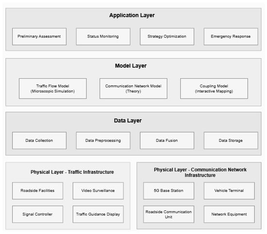
Figure 1. Overall architecture of the communication-aware DT-based RCC framework.

Table 2. Resilience assessment index system and evaluation standards.

Indicator Category	Specific Indicator	Excellent	Good	Qualified	Poor	Unit
Performance Resilience	Average Vehicle Delay Increase	<15%	15–30%	30–50%	>50%	%
	Intersection Saturation	<0.85	0.85–0.90	0.90–0.95	>0.95	–
	Maximum Queue Length	<100	100–150	150–200	>200	m
Structural Resilience	Control Node Connectivity Rate	>90%	80–90%	70–80%	<70%	%
	Communication Link Redundancy	≥3	2	1	0	links
	Backup Plan Availability	100%	80–99%	60–79%	<60%	%
Functional Resilience	Failure Detection Time	<10	10–30	30–60	>60	s
	Strategy Switching Time	<20	20–40	40–60	>60	s
	Performance Recovery Time	<5	5–10	10–15	>15	min

By integrating these dimensions, a comprehensive resilience index R is defined to evaluate the degree of performance loss and recovery speed. The calculation model for R is

$$R=1-{\displaystyle \frac{{\displaystyle {\int }_{t_0}^{t_r}\left[P_{0-p}\left(t\right)\right]dt}}{P_0(t_r-t_0)}}.$$

(8)

Here, $P_0$ represents the performance benchmark value when the system is running normally, $P_t$ represents the actual performance level of the system at time t, $t_0$ is the time when the disturbance occurs, and $t_r$ is the time when the system recovers to an acceptable performance level, and the calculation formula for intersection saturation can be expressed as

$$X_i={\displaystyle \frac{q_{i}C}{S_i{g}_i}}.$$

(9)

Here, $q_i$ is the actual traffic flow at intersection i, C is the signal period, $S_i$ is the saturation flow rate, and $g_i$ is the effective green light time. The average vehicle delay is calculated using the Webster delay model as

$$D={\displaystyle \frac{C{(1-\lambda )}^2}{2(1-\lambda X)}}+{\displaystyle \frac{X^2}{2q(1-X)}}.$$

(10)

Here, C is the signal period, $\lambda$ is the green signal ratio, X is the saturation, and q is the arrival flow rate. The first term is uniform delay and the second is random delay.

This model calculates the area under the performance loss curve and normalizes it to obtain the toughness index. The closer the R value is to 1, the stronger the system toughness. This method can reflect both the magnitude of performance degradation caused by disturbances and the speed at which the system returns to normal, providing a quantitative evaluation criterion for comparing the resilience of different control strategies.

4.2. Communication State Perception Mechanism

The communication perception mechanism monitors network status to detect quality degradation in real time. Distributed modules at the control center and roadside units collect end-to-end communication delay, packet loss, and delay jitter using 1 s probe packets. Over a sliding window of N probe packets (in our implementation, $N=10$), performance degradation is identified when the window-average communication delay exceeds the delay threshold $D_{\mathrm{th}}$ or the delay jitter exceeds a preset jitter threshold $J_{\mathrm{th}}$.

The window-average delay is computed as

$${\overline{D}}_c={\displaystyle \frac{1}{N}}\sum _{i=1}^N{D}_{c,i},$$

(11)

where $D_{c,i}$ is the measured end-to-end communication delay of the i-th probe packet. The delay jitter is defined as the standard deviation of the delay within the same window:

$$J={\sigma }_{D_c}=\sqrt{{\displaystyle \frac{1}{N}}\sum _{i=1}^N{(D_{c,i}-{\overline{D}}_c)}^2}.$$

(12)

Packet loss rate monitoring is based on a sequence number mechanism. The sender assigns a unique sequence number to each probe packet, and the receiver counts received sequence numbers and identifies missing ones, thereby computing the packet loss rate per unit time.

Due to the multidimensional characteristics of communication status, the degree of deterioration of communication quality is often difficult to describe with accurate mathematical models. Fuzzy logic can handle imprecise information and is suitable for the quantitative and qualitative assessment of communication status. Therefore, a thorough evaluation method for communication quality based on fuzzy logic was designed. The calculation model for the communication quality index (CQI) is

$$CQI=w_1{f}_d\left({\overline{D}}_c\right)+w_2{f}_l\left(L\right)+w_3{f}_j\left(J\right),$$

(13)

where ${\overline{D}}_c$ denotes the window-average end-to-end communication delay, L denotes the packet loss rate, and J denotes the delay jitter defined in (12). The functions $f_d(·)$, $f_l(·)$, and $f_j(·)$ are the corresponding membership functions, and $w_1$, $w_2$, and $w_3$ are non-negative weights satisfying $w_1+w_2+w_3=1$. The membership functions are defined as piecewise linear functions in Table 3.

Table 3. Membership function definitions for $f_d\left({\overline{D}}_c\right)$, $f_l\left(L\right)$, and $f_j\left(J\right)$.

Function		Expression	Condition
$f_d\left({\overline{D}}_c\right)$		$\left\{\begin{array}{cc}1,\hfill & {\overline{D}}_c\le 50\mathrm{ms}\hfill \\ {\displaystyle \frac{100-{\overline{D}}_c}{50}},\hfill & 50\mathrm{ms}<{\overline{D}}_c<100\mathrm{ms}\hfill \\ 0,\hfill & {\overline{D}}_c\ge 100\mathrm{ms}\hfill \end{array}\right.$	Delay membership
$f_l\left(L\right)$		$\left\{\begin{array}{cc}1,\hfill & L\le 1\%\hfill \\ {\displaystyle \frac{5-L}{4}},\hfill & 1\%<L<5\%\hfill \\ 0,\hfill & L\ge 5\%\hfill \end{array}\right.$	Loss membership
$f_j\left(J\right)$		$\left\{\begin{array}{cc}1,\hfill & J\le 10\mathrm{ms}\hfill \\ {\displaystyle \frac{50-J}{40}},\hfill & 10\mathrm{ms}<J<50\mathrm{ms}\hfill \\ 0,\hfill & J\ge 50\mathrm{ms}\hfill \end{array}\right.$	Jitter membership

Define the weight coefficients as $w_1=0.5$, $w_2=0.3$, and $w_3=0.2$. The system sets three threshold intervals for the communication quality index. When the CQI exceeds 0.8, the communication status is normal and the system runs the standard control strategy. When the CQI is between 0.5 and 0.8, the communication status slightly deteriorates and the system switches to the degraded control strategy. When the CQI is lower than 0.5, the communication status severely deteriorates and the system starts the local autonomous control mode.

To improve reproducibility, we explicitly document the CQI parameters used in all experiments ($w_1=0.5$, $w_2=0.3$, $w_3=0.2$, and thresholds $0.8/0.5$). The weights are selected to prioritize delay-related reliability because timely actuation is required in cycle-based signal control, while packet loss and jitter are incorporated as complementary indicators. In addition, we specify a one-factor-at-a-time tuning protocol around the default setting to evaluate the impact of parameter variation on the key metrics under the four scenarios.

The communication state perception mechanism also includes a communication fault prediction function, which identifies possible communication failure risks in advance by analyzing the historical evolution trend of communication performance indicators. The system adopts the ARIMA time-series prediction model, and the expression of the prediction model is

$$\begin{array}{cc}\hfill D_{t+k}=& {\varphi }_1{D}_{t+k-1}+{\varphi }_2{D}_{t+k-2}+\cdots +{\varphi }_p{D}_{t+k-p}+\hfill \\ \hfill & {\epsilon }_t-{\theta }_1{\epsilon }_{t-1}-\cdots -{\theta }_q{\epsilon }_{t-q},\hfill \end{array}$$

(14)

where $D_t$ is the observed time delay at time t, ${\varphi }_i$ and ${\theta }_i$ are model parameters and ${\epsilon }_t$ is the white noise error term.

The order of the model is determined by the following steps.

(1) Perform a stationarity test on the delayed sequence and use the augmented Dickey–Fuller (ADF) test to determine whether differential processing is necessary. After verification, the original delay sequence is non-stationary and requires first-order differencing to determine $d=1$.

(2) Draw autocorrelation function (ACF) and partial autocorrelation function (PACF) plots to analyze the autocorrelation characteristics of time delay sequences. The ACF plot shows a decay to 0 after a lag of 2 orders, while the PACF plot shows a truncation after 2 orders. The range of values for p and q has been preliminarily determined to between 1 and 3.

(3) Select the optimal model based on the Akaike Information Criterion (AIC) among the candidate models ARIMA (1,1,1), ARIMA (2,1,1), ARIMA (1,1,2), and ARIMA (2,1,2). The calculation results show that ARIMA (2,1,1) has the smallest AIC value. Therefore, $p=2$, $d=1$ and $q=1$ were ultimately determined.

Train the model parameters using the communication delay data from the past 30 min and predict the trend of delay changes in the next 5 min. When the prediction results show that the time delay will continue to rise and may exceed the threshold, the system sends an early warning signal to the control decision-making module in advance to gain a time window for the advance adjustment of the control strategy. The complete workflow of communication monitoring, fuzzy evaluation and predictive warning is shown in Figure 2. Compared to passive fault response mode, this active perception mechanism can significantly reduce the fluctuation amplitude of control performance and improve the overall resilience level of the system.

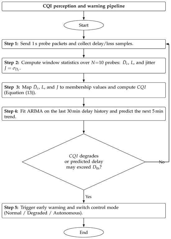
Figure 2. Flow chart of communication state perception and warning mechanism.

4.3. Adaptive Control Strategy

The adaptive control strategy dynamically adjusts signal control parameters and collaborative control modes based on real-time changes in communication and traffic conditions, achieving optimal matching between control performance and communication constraints. The strategy design follows a hierarchical control architecture, including three levels: a central coordination layer, regional control layer, and intersection execution layer. In the normal operation mode with good communication status, the central coordination layer optimizes the regional signal timing scheme based on global traffic status information using a model predictive control algorithm. The optimization objective function could be modeled as the problem

$$\begin{array}{cc}\hfill \left[\mathrm{P}1\right]:minJ& =\sum _{i=1}^N\sum _{k=1}^H\left[w_d{D}_i\left(k\right)+w_q{Q}_i\left(k\right)\right]\hfill \end{array}$$

(15a)

$$\begin{array}{cc}\hfill \mathrm{s}.\mathrm{t}.& g_{i,min}\le g_i\left(k\right)\le g_{i,max},\hfill \end{array}$$

(15b)

$$\begin{array}{cc}\hfill & \sum _{j=1}^{M_i}{g}_{i,j}\left(k\right)=C,\hfill \end{array}$$

(15c)

$$\begin{array}{cc}\hfill & Q_i(k+1)=Q_i\left(k\right)+A_i\left(k\right)-S_i\left(k\right)·g_i\left(k\right),\hfill \end{array}$$

(15d)

$$\begin{array}{cc}\hfill & 0\le Q_i\left(k\right)\le Q_{i,max}.\hfill \end{array}$$

(15e)

The prediction horizon is defined as H = 5 control cycles, which corresponds to a prediction window of 10 min under the signal cycle length C = 120 s. At each control step, the optimization problem is solved in a receding-horizon manner. Considering the nonlinear relationship between traffic states and signal timing variables, the optimization problem is solved using a sequential quadratic programming (SQP) solver embedded in the control module. The solver iteratively updates signal timing parameters while ensuring that all operational constraints are satisfied.

In addition to the bounds defined in (15b)–(15e), the following operational constraints are enforced to ensure feasible signal operations: (1) Phase order constraint: Signal phases must follow the predefined phase sequence of each intersection to prevent conflicting movements. (2) Intergreen constraint: A minimum intergreen time of 3 s is inserted between consecutive phases to guarantee traffic safety. (3) Signal timing bounds: The green duration of each phase must satisfy $g_{i,min}\le g_i\left(k\right)\le g_{i,max}$, where $g_{i,min}=15$ s and $g_{i,max}=80$ s.

Here, N is the number of intersections, H is the predicted time domain length, and $D_i\left(k\right)$ and $Q_i\left(k\right)$ represent the average delay and queue length of intersection i in the time period. k, $w_d$ and $w_q$ are weight coefficients. $g_i\left(k\right)$ is the green light duration. $g_{i,min}$ and $g_{i,max}$ are the green light duration constraints, C is the signal period, $M_i$ is the number of phases at intersection i, $A_i\left(k\right)$ is the vehicle arrival rate, $S_i\left(k\right)$ is the saturation flow rate, and $Q_{i,max}$ is the maximum queue capacity.

The estimation formula for vehicle arrival rate is

$$A_i\left(k\right)=3600{\displaystyle \frac{N_{\det }\left(k\right)}{T_{\det }}},$$

(16)

where $N_{\det }\left(k\right)$ is the number of arriving vehicles counted by the detector during the time period k, $T_{\det }$ is the detection time interval (seconds), and the coefficient 3600 is used to convert to hourly flow units. The saturation flow rate calculation formula is

$$S_i\left(k\right)=S_0{f}_w{f}_g{f}_{HV}{f}_p,$$

(17)

where $S_0$ is the introductory saturation flow rate, $f_w$ is the lane width correction factor, $f_g$ is the slope correction factor, $f_{\mathrm{HV}}$ is the significant vehicle correction factor, and $f_p$ is the parking correction factor.

The algorithm solves the optimal signal timing sequence for multiple control cycles in the future. The central coordination layer issues the optimization plan to each intersection signal for execution and updates the control decision based on dynamic changes in traffic status.

The system switches to degraded control mode when the communication status shows mild degradation. This mode reduces the communication frequency between the central coordination layer and the intersection execution layer. It changes the timing scheme from updating once every cycle to updating every three cycles, reducing the dependence on communication reliability. The algorithm for adjusting the green light duration in downgrade mode is

$$\begin{array}{cc}\hfill g_i(k+1)& =g_i\left(k\right)+\mathsf{\Delta }{g}_i\left(k\right),\hfill \end{array}$$

(18)

where $\mathsf{\Delta }{g}_i\left(k\right)$ denotes the green time adjustment, $Q_{\mathrm{threshold}}$ is the queue length threshold, and $\alpha$ is the adjustment coefficient. When $Q_i\left(k\right)>Q_{\mathrm{threshold}}$, the adjustment is given by $\mathsf{\Delta }{g}_i\left(k\right)=\alpha ·\left(Q_i\left(k\right)-Q_{\mathrm{threshold}}\right)$; otherwise, $\mathsf{\Delta }{g}_i\left(k\right)=0$. In degraded mode, the intersection controller adjusts the green time according to the queue length measured by the upstream detector. If the queue in a given direction exceeds the threshold, the green time in that direction is moderately extended to maintain an acceptable local service level. When the communication condition deteriorates severely or is completely interrupted, the system switches to local autonomous control, and each intersection operates using the locally stored timing plan without relying on the central controller or adjacent intersections. The parameter settings under different communication states are summarized in Table 4.

Table 4. Control strategy parameter configuration under different communication states.

Control Mode	Communication Quality Index	Timing Update Cycle	Coordination Range	Optimization Objective	Algorithm Complexity
Normal Mode	>0.8	1 cycle (120 s)	Full Road Network	Minimize Total Delay	High
Degraded Mode	0.5∼0.8	3 cycles (360 s)	Sub-region	Minimize Local Delay	Medium
Autonomous Mode	<0.5	Fixed Timing	Single Intersection	Balance All Phases	Low
Recovery Mode	$0.5\to 0.8$	2 cycles (240 s)	Gradually Expanding	Smooth Transition	Medium

The strategy also designs a smooth mode-switching mechanism. When the communication state gradually recovers from degradation, the system does not immediately switch back to normal mode but enters a transitional state first, gradually increasing the scope and complexity of coordinated control to prevent frequent mode switching from causing drastic fluctuations in control performance.

4.4. Fast Recovery and Optimization Algorithm

The fast recovery algorithm utilizes digital twin simulations to restore traffic status and minimize cumulative disturbance impacts. Upon detecting fault clearance, the system captures real-time vehicle distribution and queue lengths to identify priority areas for restoration. The algorithm evaluates multiple recovery strategies in a virtual environment, selecting the optimal solution to guide actual system operations. This proactive deduction ensures that control strategies are optimized for speed and efficiency during the transition back to normal service levels.

The recovery strategy adopts a phased progressive adjustment method and establishes a multi-objective optimization model. The first stage is the congestion dissipation stage, and the optimization objective is to maximize the queue dissipation rate:

$$\begin{array}{cc}\hfill \left[\mathrm{P}2\right]:\max V_{\mathrm{clear}}& =\sum _{i=1}^N{\displaystyle \frac{Q_i\left(t_0\right)-Q_i\left(t\right)}{t-t_0}}\hfill \end{array}$$

(19a)

$$\begin{array}{cc}\hfill \mathrm{s}.\mathrm{t}.& g_i\left(t\right)\le g_{i,max},\sum _{j=1}^{M_i}{g}_{i,j}\left(t\right)=C.\hfill \end{array}$$

(19b)

Here, $V_{\mathrm{clear}}$ is the queue dissipation rate, $Q_i\left(t_0\right)$ is the initial queue length at the end of the disturbance, and $Q_i\left(t\right)$ is the queue length at time t. The algorithm calculates the theoretical dissipation time based on queue length and road capacity and dynamically adjusts signal timing until the queue dissipates to a normal level. The multi-stage optimization and feedback process of the recovery algorithm is shown in Figure 3.

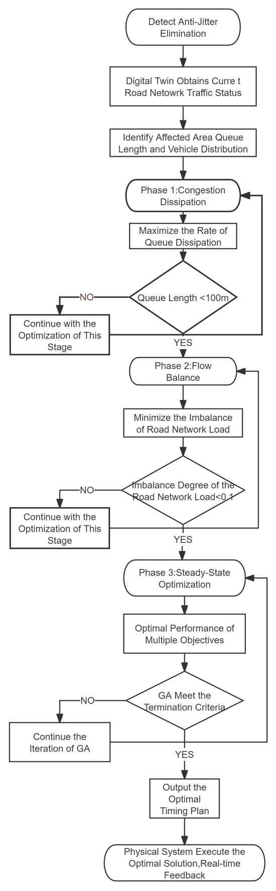
Figure 3. Flowchart of fast recovery and optimization algorithm.

The second stage is the traffic balancing stage, where the optimization objective shifts to minimizing the imbalance of road network load:

$$minU=\sum _{i=1}^N{(x_i-\overline{x})}^2.$$

(20)

The algorithm optimizes phase offsets and intersection saturation $x_i$ relative to the network average to maintain green-wave coordination, thereby reducing stops and travel time. In the steady-state stage, a genetic algorithm is employed to solve the nonlinear optimization problem. Each chromosome encodes the timing configuration of the coordinated intersections, including the signal cycle length, green splits, and phase offsets. This global search strategy helps avoid undesirable local optima and is suitable for the multi-modal objective considered here. The corresponding fitness function is defined as

$$F={\displaystyle \frac{1}{1+w_{D}D+w_{Q}Q+w_{S}S}},$$

(21)

where D, Q, and S are the road network’s average delay, queue length, and parking times, respectively.

$$\mathbf{X}=\left[C;g_0,{\varphi }_0,g_1,{\varphi }_1,\dots ,g_{M-1},{\varphi }_{M-1}\right],$$

(22)

where C is the signal cycle length, $g_i$ denotes the green split variables, and ${\varphi }_i$ denotes the offset variables.

Algorithms 1 and 2 provide the implementation details of the genetic operators used in the recovery module. Specifically, Algorithm 1 corresponds to the crossover step by exchanging selected chromosome elements, while Algorithm 2 corresponds to the mutation and feasibility-repair step used to maintain variable bounds after Gaussian perturbation.

(1) Cross exchange. For X with a length of N, perform the following swapping operation.

(2) Change and update. Perform a Gaussian transformation on every other $X\left[j\right]$. $X\left[j\right]=X\left[j\right]+\mathcal{N}\left(0,{\sigma }_m^2\right)$; $\mu$ and ${\sigma }_m^2$ are the mean and variance, and ${\sigma }_m^2$ is a Gaussian-distributed random number. This study sets ${\sigma }_m=0.1\left(X_{max}-X_{min}\right)$. $X_{max}$ and $X_{min}$ represent the maximum and minimum values in X, respectively. To implement this update and maintain variable boundaries, the corresponding matrix adjustment process can be described as follows.

Algorithm 1 Matrix element swap procedure
1: Initialize buffer $k\leftarrow \mathbf{X}\left[i\right]\left[j\right]$	▹ Buffer original value
2: Assign $\mathbf{X}\left[i\right]\left[j\right]\leftarrow \mathbf{X}\left[j\right]\left[i\right]$	▹ Execute symmetric swap
3: Update $\mathbf{X}\left[j\right]\left[i\right]\leftarrow k$	▹ Restore from buffer
4: Increment $i\leftarrow i+8$	▹ Step to next block

Algorithm 2 Matrix update and boundary adjustment
1: Aggregate $\mathbf{X}\left[i\right]\left[j\right]\leftarrow \mathbf{X}\left[i\right]\left[j\right]+\mathbf{X}\left[i\right][min(j\left)\right]$	▹ Update element value
2: Update $X_{max}\left[i\right]\leftarrow max(\mathbf{X}\left[i\right][max\left(j\right)],X_{max}\left[i\right])$	▹ Adjust upper bound
3: Update $X_{min}\left[i\right]\leftarrow min(\mathbf{X}\left[i\right][min\left(j\right)],X_{min}\left[i\right])$	▹ Adjust lower bound

The genetic algorithm initializes a population of 50 chromosomes encoding signal cycles, green splits, and offsets and evaluates their fitness via digital twin simulations. It employs tournament selection, single-point crossover, and Gaussian mutation and terminates after 100 generations or when the improvement in the best fitness value becomes negligible. In the current implementation, the crossover and mutation rates are fixed according to the simulation setting used in the code, and the same random-seed control is applied across repeated runs to ensure reproducibility of the recovery optimization results. To accelerate convergence, a case library stores historical traffic vectors, including flow, saturation, and queue lengths, so as to provide high-quality starting points for the algorithm. The similarity between the current traffic scenario and historical cases in the case library is calculated through cosine similarity.

$$\rho ={\displaystyle \frac{X·Y}{\parallel X\parallel \parallel Y\parallel }}.$$

(23)

The feature vector X comprises flow Q, saturation S, and queue length L for n intersections. If the cosine similarity $\rho$ between current and historical vectors exceeds 0.85, the system populates 30% of the initial genetic algorithm population with stored solutions to accelerate convergence, while randomly generating the remainder to preserve diversity. The threshold $\rho =0.85$ is selected as a compromise between solution reuse and population diversity: a lower threshold may introduce cases that are not sufficiently similar to the current traffic state, while a higher threshold may excessively reduce the number of reusable high-quality initial solutions. In the present manuscript, this threshold is used as the default initialization criterion in the recovery module, while a more exhaustive threshold sensitivity evaluation is left for future extended experiments.

$$E\left(t\right)=\left|P_{\mathrm{target}}-P_{\mathrm{actual}}\left(t\right)\right|,$$

(24)

where $P_{\mathrm{target}}$ represents the target performance level, while $P_{\mathrm{actual}}\left(t\right)$ represents the actual performance level. When $E\left(t\right)$>20%, trigger strategy reassessment and adjust subsequent recovery strategies in the digital twin environment to ensure that the system can converge to the target state robustly.

5. System Implementation and Simulation Verification

The joint simulation platform couples SUMO and NS-3 through a bidirectional interface to verify the communication-aware control system. The overall architecture of the joint simulation platform is illustrated in Figure 4. SUMO models the transportation hub’s microscopic traffic, simulating 8000 vehicles per hour across major roads and outputting real-time status data. Simultaneously, NS-3 reproduces a 5G network environment, calculating dynamic latency and packet loss based on a 100 Mbps bandwidth and the TCP/IP protocol. The interface synchronizes these environments every second, allowing communication performance to directly influence signal control strategies. A digital twin module visualizes trajectories and link states while recording data for performance analysis on a high-performance workstation.

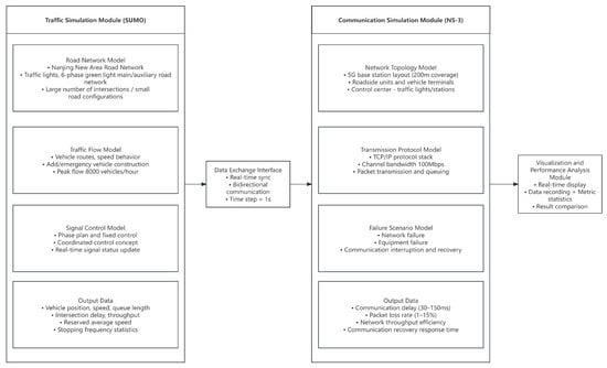
Figure 4. Schematic diagram of the architecture of the joint simulation platform.

Experimental Design and Parameter Setting

This study compares four control schemes, which can be expressed as fixed-time, traditional SCOOT, communication-aware without recovery (CAwR) and the proposed RCC. These schemes are tested across four scenarios: normal operation, mild degradation, severe degradation, and a complete interruption–recovery cycle. The interruption scenario simulates a 40 min event with complete loss, partial restoration, and full recovery. Experiments are conducted with a 10 min warm-up and five repetitions to ensure data reliability.

To ensure a fair comparison, all schemes share the same road network, demand profiles, detector settings, signal cycle length, and green bounds as listed in Table 5. The SCOOT baseline is implemented as an adaptive split/offset update driven by detector measurements with the same control cycle and the same operational constraints as the proposed method. To ensure fairness under communication degradation, SCOOT command delivery is subject to the same NS-3 modeled delay and packet loss, and the executed timing plan at each intersection follows the same actuation timing as other centralized schemes.

Table 5. Simulation and communication parameter settings used in the evaluation.

Parameter Name	Symbol	Value Setting	Unit
Simulation Area	$A_{\mathrm{net}}$	$4\times 3$	${\mathrm{km}}^2$
Number of Intersections	$N_{\mathrm{int}}$	8	–
Total Road Length	$L_{\mathrm{road}}$	15.6	km
Peak Hour Traffic Flow	$Q_{\mathrm{peak}}$	8000	vehicles/hour
Average Vehicle Length	$l_{\mathrm{veh}}$	4.5	m
Maximum Driving Speed	$v_{max}$	60	km/h
Signal Cycle Length	C	120	s
Minimum Green Time	$g_{min}$	15	s
Maximum Green Time	$g_{max}$	80	s
Normal Communication Delay	$D_{\mathrm{norm}}$	30–50	ms
Degraded Communication Delay	$D_{\mathrm{deg}}$	60–150	ms
Normal Packet Loss Rate	$L_{\mathrm{norm}}$	<1	%
Degraded Packet Loss Rate	$L_{\mathrm{deg}}$	2–12	%
Total Simulation Duration	$T_{\mathrm{sim}}$	60	min
Warm-up Time	$T_{\mathrm{warm}}$	10	min
Number of Repetitions	$N_{\mathrm{rep}}$	5	times

Table 5 lists the specific road network, signal control, and 5G communication parameters used in the evaluation.

Primarily, the proposed RCC outperforms the compared strategies across all reported scenarios. In Table 6, the Proposed RCC column is reported as mean ± standard deviation over $N_{\mathrm{rep}}=5$ independent runs, whereas the baseline columns retain the corresponding comparison values under the same scenario settings. Under normal operation, the proposed RCC achieves the lowest average delay and the highest network average speed among the compared schemes. Under severe degradation, it maintains lower delay and higher speed than SCOOT, which does not explicitly account for communication degradation. During the interruption–recovery process, the DT-supported recovery mechanism yields the shortest recovery time and the highest resilience index among the compared methods. The detailed numerical results are summarized in Table 6 and Figure 5.

Table 6. Performance comparison results of various schemes under different scenarios. The Proposed RCC column is reported as mean ± standard deviation over $N_{\mathrm{rep}}=5$ runs, while the baseline columns retain the corresponding comparison values.

Scenario	Metric	Fixed-Time	SCOOT	CAwR	Proposed RCC
Normal	Average delay (s)	59.1	43.8	43.2	$42.3\pm 0.8$
Normal	Avg. speed (km/h)	32.5	35.2	35.6	$36.1\pm 0.4$
Mild degradation	Average delay (s)	59.8	78.5	62.4	$51.7\pm 1.4$
Mild degradation	Avg. speed (km/h)	32.1	26.3	30.8	$33.4\pm 0.5$
Severe degradation	Average delay (s)	60.5	96.8	68.3	$55.9\pm 1.8$
Severe degradation	Avg. speed (km/h)	31.8	21.4	28.5	$32.6\pm 0.5$
Interruption–recovery	Recovery time (min)	12.6	8.4	4.7	$4.7\pm 0.3$
Interruption–recovery	Resilience index	0.52	0.31	0.68	$0.87\pm 0.02$

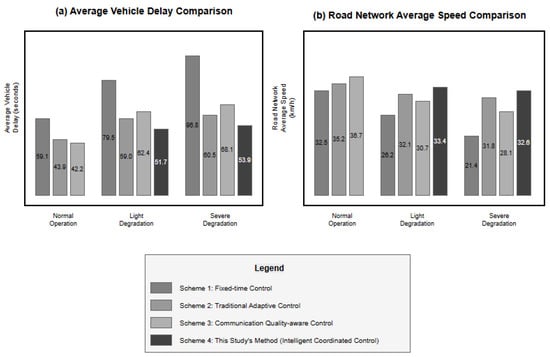
Figure 5. Performance comparison of different control schemes in communication degradation scenarios. The plotted values correspond to the comparative results under the representative scenarios, while the proposed RCC results are reported in Table 6 as mean ± standard deviation over $N_{\mathrm{rep}}=5$ runs. Legend mapping: Scheme 1 = fixed-time; Scheme 2 = SCOOT; Scheme 3 = CAwR; and Scheme 4 = proposed RCC.

All experiments are repeated $N_{\mathrm{rep}}=5$ times with different random seeds. In Table 6, the Proposed RCC column is reported as mean ± standard deviation over the five runs, while the baseline columns retain the corresponding comparison values under the same scenario settings, i.e., $\overline{x}={\displaystyle \frac{1}{N_{\mathrm{rep}}}}{\sum }_{r=1}^{N_{\mathrm{rep}}}{x}_r,s=\sqrt{{\displaystyle \frac{1}{N_{\mathrm{rep}}-1}}{\sum }_{r=1}^{N_{\mathrm{rep}}}{(x_r-\overline{x})}^2}.$ When needed, a two-sided 95% confidence interval is computed as $\overline{x}\pm t_{0.975,N_{\mathrm{rep}}-1}{\displaystyle \frac{s}{\sqrt{N_{\mathrm{rep}}}}}$.

Table 6 focuses on the core benchmarking results of the compared control schemes under the representative scenarios listed in Table 5. The present manuscript does not include a full parameter sensitivity analysis or a component-wise ablation evaluation; these are left for future extended experiments.

6. Discussion

6.1. Computational Overhead

The online RCC loop consists of CQI computation, mode switching, and (in normal mode) MPC updates once per signal cycle. The main computational burden arises during recovery, where the DT-supported GA evaluates candidate timing plans via simulation rollouts. In practice, this overhead can be controlled by limiting GA population size and generations and by restricting optimization to affected sub-regions.

6.2. Scalability Beyond 8 Intersections

Although the current evaluation considers an eight-intersection hub network, the RCC framework is compatible with hierarchical scaling. A practical approach is to partition the network into regions and apply coordination within regions under degraded communication, while maintaining local autonomous control at intersection level when CQI is poor. This limits the decision dimension and communication dependency as network size increases.

6.3. Limitations and Transferability

This study is validated using SUMO–NS-3 co-simulation and assumes consistent detector availability and a modeled protocol stack. Real-world deployments may involve sensing faults, non-stationary demand, heterogeneous roadside equipment, and implementation constraints that are not fully captured. Future work will focus on field data calibration or hardware-in-the-loop testing and on evaluating real-time deployment overhead.

Another limitation of the current study is that a systematic parameter sensitivity analysis and a component-wise ablation study are not yet included. Although the main comparative results already indicate the effectiveness of the proposed RCC under representative communication degradation scenarios, a more exhaustive evaluation of module-wise contributions and parameter robustness is left for future work.

7. Conclusions

This study proposes a resilient collaborative control (RCC) method for transportation hubs based on a communication-aware digital twin architecture. By integrating real-time communication state perception, adaptive mode switching, and DT-supported recovery optimization, the proposed framework aims to improve the robustness of traffic signal control under communication degradation. All evidence reported in this paper is obtained from the SUMO–NS-3 co-simulation platform and the configured scenarios described in Section 5. Within this simulation setting, the results indicate that, compared with traditional adaptive control, the proposed method reduces average vehicle delay by 42.3%, increases network speed by 52.3%, shortens recovery time by 63%, and improves the resilience index to 0.87. These findings should therefore be interpreted within the scope of the evaluated co-simulation setting.

References

- Cui, H.; Dong, X.; Su, Y.; Zhu, M.; Ma, X. Exploring spatiotemporal patterns of frequently congested urban road segments based on multi-source data: A case study of China’s super-large cities. Transp. Res. Rec. 2024, 2678, 2077–2093. [Google Scholar] [CrossRef]
- Wei, X.; Ren, Y.; Shen, L.; Shu, T. Exploring the spatiotemporal pattern of traffic congestion performance of large cities in China: A real-time data based investigation. Environ. Impact Assess. Rev. 2022, 95, 106808. [Google Scholar] [CrossRef]
- Wu, K.; Ding, J.; Lin, J.; Zheng, G.; Sun, Y.; Fang, J.; Xu, T.; Zhu, Y.; Gu, B. Big-data empowered traffic signal control could reduce urban carbon emission. Nat. Commun. 2025, 16, 2013. [Google Scholar] [CrossRef]
- Agafonov, A.; Yumaganov, A.; Myasnikov, V. Adaptive Traffic Signal Control by Choosing Phase Duration. In Proceedings of the 2024 X International Conference on Information Technology and Nanotechnology (ITNT), Samara, Russia, 20–24 May 2024; IEEE: Piscataway, NJ, USA, 2024; pp. 1–4. [Google Scholar] [CrossRef]
- Rasheed, F.; Yau, K.-L.A.; Noor, R.M.; Wu, C.; Low, Y.-C. Deep reinforcement learning for traffic signal control: A review. IEEE Access 2020, 8, 208016–208044. [Google Scholar] [CrossRef]
- Finkelberg, I.; Petrov, T.; Gal-Tzur, A.; Zarkhin, N.; Počta, P.; Kováčiková, T.; Buzna, L.; Dado, M.; Toledo, T. The effects of vehicle-to-infrastructure communication reliability on performance of signalized intersection traffic control. IEEE Trans. Intell. Transp. Syst. 2022, 23, 15450–15461. [Google Scholar] [CrossRef]
- Wang, X.; Garg, S.; Lin, H.; Kaddoum, G.; Hu, J.; Hassan, M.M. Heterogeneous Blockchain and AI-Driven Hierarchical Trust Evaluation for 5G-Enabled Intelligent Transportation Systems. IEEE Trans. Intell. Transp. Syst. 2023, 24, 2074–2083. [Google Scholar] [CrossRef]
- Das, D.; Rana, M.K.; Sardar, B.; Pecorella, T.; Saha, D. A Comparative Analysis of Distributed Mobility Management Schemes for 5G-Based Intelligent Transportation Systems. IEEE Trans. Intell. Transp. Syst. 2025, 26, 2434–2448. [Google Scholar] [CrossRef]
- Alalewi, A.; Dayoub, I.; Cherkaoui, S. On 5G-V2X use cases and enabling technologies: A comprehensive survey. IEEE Access 2021, 9, 107710–107737. [Google Scholar] [CrossRef]
- Singh, D.; Taj, A.; Yadav, D.; Yadav, E.S.; Jayaswal, V.; Sharma, J. Adaptive Traffic Signal Timer for Traffic Control System Using Artificial Intelligence. In Proceedings of the 2025 3rd International Conference on Communication, Security, and Artificial Intelligence (ICCSAI), Greater Noida, India, 4–6 April 2025; IEEE: Piscataway, NJ, USA, 2025; Volume 3, pp. 2153–2156. [Google Scholar] [CrossRef]
- Adarbah, H.Y.; Sookhak, M.; Atiquzzaman, M. A digital twin-based traffic light management system using BIRCH algorithm. Ad Hoc Netw. 2024, 164, 103613. [Google Scholar] [CrossRef]
- Zhu, H.; Sun, F.; Tang, K.; Wu, H.; Feng, J.; Tang, Z. Digital twin-enhanced adaptive traffic signal framework under limited synchronization conditions. Sustainability 2024, 16, 5502. [Google Scholar] [CrossRef]
- Kumarasamy, V.K.; Saroj, A.J.; Liang, Y.; Wu, D.; Hunter, M.P.; Guin, A.; Sartipi, M. Integration of decentralized graph-based multi-agent reinforcement learning with digital twin for traffic signal optimization. Symmetry 2024, 16, 448. [Google Scholar] [CrossRef]
- Li, H.; Zhang, Q.; Wu, L.; Zhang, Z. Impact of communication performance measures for the Internet of Vehicles in an intersection scenario. Simul. Model. Pract. Theory 2025, 140, 103086. [Google Scholar] [CrossRef]
- Balke, K.; Sunkari, S.; Florence, D.; Tantillo, M.J.; Lawrence, C. Traffic Signal Program Handbook; Technical Report; Department of Transportation, Federal Highway Administration: Washington, DC, USA, 2023. [Google Scholar]
- Yau, K.-L.A.; Qadir, J.; Khoo, H.L.; Ling, M.H.; Komisarczuk, P. A survey on reinforcement learning models and algorithms for traffic signal control. ACM Comput. Surv. (CSUR) 2017, 50, 1–38. [Google Scholar] [CrossRef]
- Gao, Y.; Qian, S.; Li, Z.; Wang, P.; Wang, F.; He, Q. Digital twin and its application in transportation infrastructure. In Proceedings of the 2021 IEEE 1st International Conference on Digital Twins and Parallel Intelligence (DTPI), Beijing, China, 15 July–15 August 2021; IEEE: Piscataway, NJ, USA, 2021; pp. 298–301. [Google Scholar]
- Cai, B.; Xie, M.; Liu, Y.; Liu, Y.; Feng, Q. Availability-based engineering resilience metric and its corresponding evaluation methodology. Reliab. Eng. Syst. Saf. 2018, 172, 216–224. [Google Scholar] [CrossRef]
- Wu, D.; Zheng, A.; Yu, W.; Cao, H.; Ling, Q.; Liu, J.; Zhou, D. Digital twin technology in transportation infrastructure: A comprehensive survey of current applications, challenges, and future directions. Appl. Sci. 2025, 15, 1911. [Google Scholar] [CrossRef]
- Zhou, Y.; Wang, J.; Yang, H. Resilience of transportation systems: Concepts and comprehensive review. IEEE Trans. Intell. Transp. Syst. 2019, 20, 4262–4276. [Google Scholar] [CrossRef]
- Yan, B.; Yang, F.; Qiu, S.; Wang, J.; Cai, B.; Wang, S.; Zaheer, Q.; Wang, W.; Chen, Y.; Hu, W. Digital twin in transportation infrastructure management: A systematic review. Intell. Transp. Infrastruct. 2023, 2, liad024. [Google Scholar] [CrossRef]
- Ge, C.; Qin, S. Digital twin intelligent transportation system (DT-ITS)—A systematic review. IET Intell. Transp. Syst. 2024, 18, 2325–2358. [Google Scholar] [CrossRef]
- Djordjević, B.; Krmac, E.; Lin, C.-Y.; Fröidh, O.; Kordnejad, B. An optimisation-based digital twin for automated operation of rail level crossings. Expert Syst. Appl. 2024, 239, 122422. [Google Scholar] [CrossRef]
- An, C.; Wu, Y.-J.; Xia, J.; Lu, Z. Investigating impacts of communication loss on signal performance with use of event-based data. Transp. Res. Rec. 2017, 2645, 38–49. [Google Scholar] [CrossRef]
- Wang, M.I.-C.; Wen, C.H.-P.; Chao, H.J. Assessing the impact of communication delays for Autonomous Intersection Management systems. Veh. Commun. 2024, 49, 100829. [Google Scholar] [CrossRef]
- Zeinaly, Z.; Sojoodi, M.; Bolouki, S. A resilient intelligent traffic signal control scheme for accident scenario at intersections via deep reinforcement learning. Sustainability 2023, 15, 1329. [Google Scholar] [CrossRef]
- Rodrigues, F.; Azevedo, C.L. Towards robust deep reinforcement learning for traffic signal control: Demand surges, incidents and sensor failures. In Proceedings of the 2019 IEEE Intelligent Transportation Systems Conference (ITSC), Auckland, New Zealand, 27–30 October 2019; IEEE: Piscataway, NJ, USA, 2019; pp. 3559–3566. [Google Scholar]
- Petrov, T.; Finkelberg, I.; Počta, P.; Buzna, L.; Zarkhin, N.; Gal-Tzur, A.; Toledo, T. An analytical approach to the estimation of vehicular communication reliability for intersection control applications. Veh. Commun. 2024, 45, 100693. [Google Scholar] [CrossRef]
- Grieves, M.; Vickers, J. Digital twin: Mitigating unpredictable, undesirable emergent behavior in complex systems. In Transdisciplinary Perspectives on Complex Systems: New Findings and Approaches; Springer: Berlin/Heidelberg, Germany, 2016; pp. 85–113. [Google Scholar]
- Hosseini, S.; Barker, K.; Ramirez-Marquez, J.E. A review of definitions and measures of system resilience. Reliab. Eng. Syst. Saf. 2016, 145, 47–61. [Google Scholar] [CrossRef]
- Yao, K.; Chen, S. Resilience-based adaptive traffic signal strategy against disruption at single intersection. J. Transp. Eng. Part A Syst. 2022, 148, 04022018. [Google Scholar] [CrossRef]
- Toroghi, S.S.H.; Thomas, V.M. A framework for the resilience analysis of electric infrastructure systems including temporary generation systems. Reliab. Eng. Syst. Saf. 2020, 202, 107013. [Google Scholar] [CrossRef]
Disclaimer/Publisher’s Note: The statements, opinions and data contained in all publications are solely those of the individual author(s) and contributor(s) and not of MDPI and/or the editor(s). MDPI and/or the editor(s) disclaim responsibility for any injury to people or property resulting from any ideas, methods, instructions or products referred to in the content. |
© 2026 by the authors. Licensee MDPI, Basel, Switzerland. This article is an open access article distributed under the terms and conditions of the Creative Commons Attribution (CC BY) license.