Weak Signal Detection Method for Millimeter-Wave Sensor Signals Based on Heterodyne Duffing Oscillator

Abstract

Millimeter-wave technology helps achieve antenna miniaturization and high gain, but it is limited by factors such as short wavelength, high transmission loss, and high signal-to-noise ratio, which put higher requirements on the accuracy and computing speed of signal processing methods. The weak signal detection method based on the Duffing oscillator is suitable for detecting and estimating the parameters of such signals, but its intermittent chaotic state brings difficulties in phase determination and limited frequency detection accuracy. This article proposes a Heterodyne Duffing equation, which analyzes system properties through bifurcation diagrams, timing diagrams, and phase diagrams. Based on this, signal detection and frequency estimation models are designed, and frequency detection accuracy and calculation time are discussed. The analysis and simulation results show that the phase state discrimination speed and accuracy of the Heterodyne Duffing oscillator (HDO) are superior to the traditional Duffing equation-based intermittent chaotic state method. It has adjustable frequency resolution, overcomes the inherent 0.03ω frequency detection error limitation of the traditional Duffing oscillator, and has a significant advantage in phase state discrimination speed. The frequency estimation method based on the proposed HDO can better meet the frequency resolution and real-time requirements of millimeter-wave sensor signals.

1. Introduction

The advancement of millimeter-wave (mmWave) technology has accelerated the application of mmWave sensors in global military sensor systems [1,2], making it one of the key development directions for ammunition radio sensors for various military powers. Accurate frequency measurement is essential for effectively jamming such sensors. However, due to inherent signal propagation characteristics, millimeter-wave signal detection faces significant challenges. According to the free-space transmission loss formula of signals, signal transmission loss is related to distance and frequency. The farther the distance, the higher the frequency, and the greater the transmission loss. Therefore, there are two difficulties in signal detection for millimeter-wave sensors: Firstly, the signal duration is short. The sensor may only operate for tens of milliseconds to a few seconds, and the signal duration is very short, which requires high real-time performance for signal detection. Secondly, there is severe propagation loss. Millimeter-wave sensor signals have low power consumption and high spatial propagation loss, especially for radio sensors in the V/W band. At the same distance and transmission power, the attenuation of 80 GHz f-band millimeter signals is 24 dB higher than that of 10 GHz x-band signals, resulting in an extremely low received signal-to-noise ratio (SNR), which places stringent requirements on the detection capability of the receiver.

Considering the high real-time detection requirements of millimeter-wave-induced signals and the bad signal-to-noise ratio, the weak signal detection and parameter estimation method based on chaos theory can be used to solve these problems. Since Feigenbaum, an American scholar, established the principle of chaos universality in the 1970s, pushing chaos from qualitative analysis to quantitative calculation has played a positive role in the application, research, and development of chaos and nonlinear systems. As an example, the Duffing oscillator was first proposed by Birx [3] for weak signal detection in 1992. Subsequently, Wang Guanyu et al. [4] of Zhejiang University analyzed the basic principle of the Duffing oscillator for simple weak signal detection, and improved the Duffing oscillator to detect periodic signals with different frequencies. Although the signal form is still simple, this method outperforms traditional methods in terms of computational speed and minimum detectable signal-to-noise ratio. Since then, a weak signal detection method based on chaos theory has attracted the attention of many scholars. The weak signal detection method based on the chaos system is mainly divided into the following three research directions [5]: one is to extract useful signals under the background of chaotic noise by predicting the chaotic model; the second is to use the chaotic characteristics for high-precision “chaotic” measurement; the third is to use the initial value sensitivity and noise immunity of the chaotic system to detect weak signals based on the phase change of the chaotic oscillator, also a hotspot in the current chaos detection field.

Several typical chaotic dynamical systems which are widely used in the chaos detection method include the Lorenz model, Rossler model, Logistic map, Van der Pol oscillator, and Duffing oscillator [6]. Compared with the first four models, the Duffing oscillator is the most popular model in current studies. For example, in 2003, Li Yue et al. [7] proposed a new detection model based on the modified nonlinear term of the Duffing equation and experimentally verified that the model can obtain better detection results than previous ones at low SNRs. Hou et al. [8] proposed a weak broadband signal detection method based on the Duffing oscillator, which achieved accurate detection of chirp and other signals when the signal-to-noise ratio was not lower than −20 dB. Cheng et al. [9] proposed a frequency-locking principle by using intermittent chaotic periodic characteristics and introduced an array of chaotic oscillators for weak signal detection at unknown frequencies. The key to the method of signal detection and parameter estimation based on the extended Duffing system is to distinguish the intermittent chaotic state of the system. Due to the alternating appearance of periodic and chaotic states in intermittent chaotic states, traditional methods for distinguishing intermittent chaotic states can only be based on a time series that reflects the system’s motion state for phase discrimination, that is, the average motion state of the system during this period, which makes intermittent chaotic states easy to misjudge. Therefore, the existing chaotic methods suffer from low accuracy and efficiency in phase discrimination and critical threshold determination.

Traditionally, methods based on time–frequency analysis are commonly used to process millimeter-wave signals. These include the short-time Fourier transform (STFT), Wigner distribution [10], smooth pseudo-Wigner distribution [11], and fractional Fourier transform as well as a combination of these methods [12,13] to conduct signal parameter analysis. Reference [14] developed a parameterized centroid frequency–chirp rate distribution (PCFCRD) approach for analyzing multicomponent linear frequency modulation (LFM) signals. By introducing a fixed time delay, the method mitigates noise correlation and achieves improved estimation accuracy even at an SNR of −12 dB. The short-time fractional Fourier transform (FrFT) has recently seen significant theoretical extensions, such as its integration with time series prediction [15], transformer encoders [16], and graph signal processing [17]. In the specific context of sensor-based detection, Chen et al. [18] applied the short-time FrFT to extract micro-Doppler (m-D) features of moving targets within spiky sea clutter. This mechanism determines the presence of micro-motion targets in the optimal FrFT domain, maintaining a high detection probability even at a low SNR of −5 dB. Regarding parameterized time–frequency analysis, Yang et al. [19] provided a comprehensive review of its engineering applications. Subsequent studies have focused on optimizing specific mechanisms. For instance, Zhao et al. [20] and Guan et al. [21] advanced chirplet transforms to handle nonstationary fault features and crossing frequency trajectories, respectively. Furthermore, Hatano et al. [22] explored sparse atomic decomposition, while Wang et al. [23] and Chen et al. [24] developed generalized parameterized transforms to improve Direction-of-Arrival (DOA) estimation and multi-squeezing performance.

Although parameter estimation based on time–frequency analysis has advanced significantly, accurate detection in low-SNR environments remains a bottleneck due to the threshold effect. Hu et al. [25] utilized the smoothed pseudo-Wigner–Ville distribution (SPWVD) and density peak clustering for modal estimation. While this method achieved high accuracy, its validation was primarily concentrated on high-SNR scenarios within 5 dB to 15 dB SNRs, leaving its robustness in strong noise unverified. Similarly, Li et al. [26] proposed the window Radon Fractional Fourier transform (WRFRFT) to address Doppler spread effects. Although WRFRFT outperforms the standard Radon Fractional Fourier transform, quantitative results indicate that its estimation performance deteriorates significantly when the SNR drops below −10 dB [26]. This degradation occurs because the cross-terms and noise floor in traditional time–frequency distributions mask the target energy at extremely low SNRs [27]. On the other hand, chaos-based approaches, such as combining the Duffing oscillator with wavelet analysis [28,29], demonstrate superior noise immunity. However, these methods are currently limited to detecting low-frequency signals and struggle to cover the wide bandwidth required for radar sensor applications. Consequently, existing methods either suffer from the SNR threshold limitation below −10 dB or lack the frequency adaptability for millimeter-wave sensing.

In response to these issues, our study proposes a new Heterodyne Duffing oscillator (HDO) model, which makes the discrimination of the system more accurate and efficient, and the accuracy of the critical threshold is also significantly improved. Based on this method, this paper further studies the signal frequency estimation based on the HDO, and analyzes its frequency resolution and real-time performance. Meanwhile, based on the weak signal detection model of the HDO, this paper proposes a parameter estimation method for LFM signals under low-SNR conditions, and verifies the accuracy of its parameter estimation through simulation.

Here is the overall structure of this paper. Section 2 presents the weak signal detection mechanism of the classical Holmes-type Duffing equation and analyzes the two most critical issues: intermittent chaos generation and the phase state discrimination method. Section 3 proposes a HDO and analyzes its properties. Section 4 presents a signal frequency estimation method based on the proposed system, and analyzes frequency resolution and real-time performance. Section 5 presents a frequency estimation method for LFM signals based on the proposed system. Section 6 concludes our study.

2. Weak Signal Detection Model of Duffing Oscillator

The expression for a Holmes-type Duffing oscillator is as follows:

$$\ddot{x}(t)+k\dot{x}(t)-x(t)+x^3(t)=F\cos (\omega t)$$

(1)

where $x$ stands for the displacement,$t$ is the time, k represents the damping ratio, $-x+x^3$ is the combined restoring force, which includes both a linear component and a nonlinear cubic component, and $Fcos\left(\omega t\right)$ is the periodic internal driving force. We use phase diagrams to demonstrate its typical properties. The Duffing oscillator will go through the small-period oscillatory motion, the homogeneous orbital motion, the multiplicative-period bifurcation motion, the chaotic motion, and the large-scale periodical motion in sequence, as shown in Figure 1.

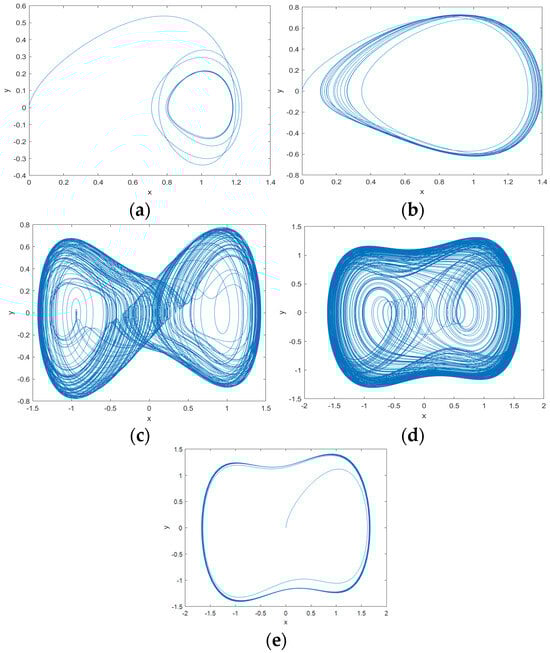
Figure 1. Phase plane trajectories of Duffing oscillator output when amplitudes of periodic internal curved force signals are different: (a) $F=0.2$, Duffing oscillator in small-period oscillation motion; (b) $F=0.35$, Duffing oscillator in homolithic orbital motion; (c) $F=0.4$, Duffing oscillator in doubly periodic bifurcation motion; (d) $F=0.8$, Duffing oscillator in chaotic motion; (e) $F=0.827$, Duffing oscillator in large-scale periodic motion.

Setting the system close to the critical chaotic state, Figure 2 compares the phase diagrams of the system output under different system inputs, namely adding only strong noise and adding only weakly periodic signals with noise. It can be seen that adding noise alone cannot cause a phase transition in the system, but adding a weak signal with noise can cause a phase transition in the system. This indicates that oscillators possess the characteristic of high sensitivity to dynamic signals and robustness to zero mean noise, which enables them to effectively detect and estimate weak periodic signal parameters under low-SNR conditions.

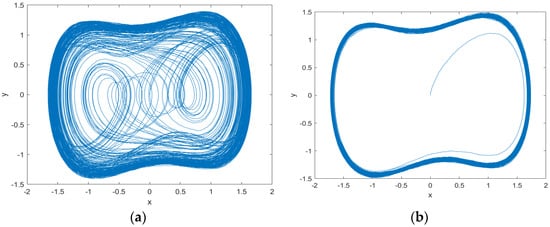
Figure 2. Phase plane trajectories of the system output after different signals are input into the chaotic Duffing oscillator: (a) with strong noise added only; (b) with a weak signal and strong noise added at the same time.

It is necessary to transform the Duffing oscillator equation by using the scale transformation method and adding the noisy signal to be measured. The state equation expression is as follows:

$$\left\{\begin{array}{l}\dot{x}=\omega y\\ \dot{y}=\omega \left(-ky+x-x^3+F\cos (\omega t)+A\cos ({\omega }_{0}t+{\phi }_0)+n(t)\right)\end{array}\right.$$

(2)

In the equation, $A\cos ({\omega }_{0}t+{\phi }_0)$ denotes the input weak signal to be measured, and $n\left(t\right)$ represents the noise signal. Equation (2) is the commonly used extended Duffing oscillator weak signal detection model, as it provides a general expression form of the Duffing equation under different periodic internal driving force frequencies [3]. The general steps for signal detection of this model are as follows: First, adjust its internal driving force signal amplitude to a critical threshold; that is, adjust the amplitude to the critical threshold $F_c$. According to the Melnikov method and bifurcation analysis [3,5], the critical threshold for the transition from chaotic motion to periodic motion is typically determined as $F_c\approx 0.826$, so that it is in a borderline chaotic state. Then, input the signal to be tested into the system. If the oscillator undergoes a phase transition, it is considered that the signal to be tested contains the target signal.

2.1. Intermittent Chaotic State

To discuss the reasons for the emergence of intermittent chaotic states, Equation (2) needs to be analyzed. Without considering the noise, the total cranking power signal can be equivalently expressed as

$$F_{\mathrm{c}}\cos (\omega t)+A\cos ({\omega }_{0}t+{\phi }_0)=F_{\mathrm{e}}(t)\cos (\omega t+\Phi (t))$$

(3)

In

$$F_{\mathrm{e}}(t)=\sqrt{{F_{\mathrm{c}}}^2+2F_{\mathrm{c}}A\cos (\Delta \omega t+{\phi }_0)+A^2}$$

(4)

$$\Phi (t)=\arctan {\displaystyle \frac{A\sin (\Delta \omega t+{\phi }_0)}{F_{\mathrm{c}}+A\cos (\Delta \omega t+{\phi }_0)}}$$

(5)

$F_e\left(t\right)$ represents the system equivalent driving force signal amplitude.$\Delta \omega$ is the frequency difference between the signal under measurement and the periodic internal driving force, $|\Delta \omega | = |{\omega }_0-\omega |$. Since the amplitude of the signal under measurement is usually much smaller than the amplitude of the internal driving force signal, $\Phi \left(t\right)$ can be ignored.

In practical applications, it is very unlikely that the frequency of the periodic internal driving force of the Duffing oscillator is exactly equal to the frequency of the signal to be measured, and there is often a slight error between them; that is, $\Delta \omega \ne 0$. At this time, $F_e\left(t\right)$ will vary with the difference frequency $\mathsf{\Delta }\omega$, and its vector relationship is shown in Figure 3.

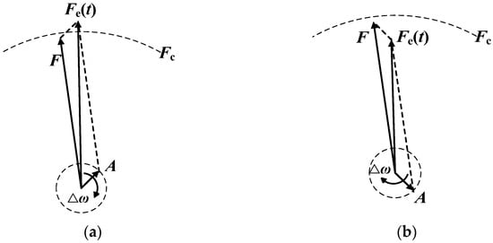
Figure 3. Vector diagram of the relationship between the amplitude of the equivalent driving force signal of the Duffing oscillator and the critical threshold of the system: (a) $F_e\left(t\right)>F_c$; (b) $F_e\left(t\right)<F_c$.

In Figure 3a, when the direction of the target signal is consistent with the driving force signal within the system, the amplitude of the equivalent driving force signal Fe(t) resulting from the combination of the two will be greater than the critical threshold Fc of the system; that is, $F_e\left(t\right)>F_c$. At this point, the Duffing oscillator will transform from chaotic motion to large-scale periodic motion. $F_e\left(t\right)$ will gradually change over time. Therefore, after a period of time, the directions of the vector of the target signal and the driving force signal within the system will gradually deviate, as shown in Figure 3b. $F_e\left(t\right)$ will gradually become lower than $F_c$, and at this point, the system will reconvert from the large-scale periodic state to the chaotic state. This regular periodic alternation process of the Duffing oscillator between the chaotic state and the large-scale periodic state over time is the intermittent chaotic motion of the Duffing oscillator, as shown in Figure 4.

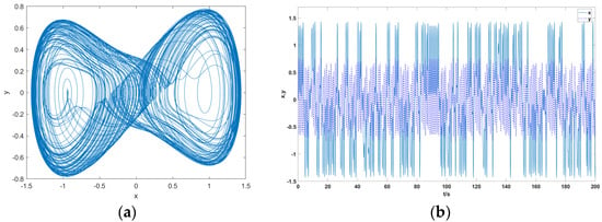
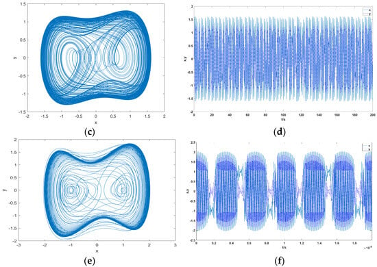
Figure 4. Vector diagram of the relationship between the amplitude of the equivalent driving force signal of the Duffing oscillator and the critical threshold of the system: (a) phase plane trajectory, double-period bifurcation motion; (b) time domain waveform, double-period bifurcation motion; (c) phase plane trajectory, chaotic motion; (d) time domain waveform, chaotic motion; (e) phase plane trajectory, intermittent chaotic state; (f) time domain waveform, intermittent chaotic state.

As shown in Figure 4, as the amplitude F of the internal control force signal continuously increases, the Holmes-type Duffing oscillator exhibits different dynamic characteristics. When 0.826 > $F_e\left(t\right)$ > 0.38, as $F_e\left(t\right)$ increases, the Duffing oscillator transitions from the double-period bifurcation motion state to the chaotic motion state. When $F_e\left(t\right)$ is at the critical value of 0.826, it will show periodic characteristics, but when $|\Delta \omega |$ is too large, because the durations of $F_e\left(t\right)>F_c$ and $F_e\left(t\right)<F_c$ are too short to maintain the stable large-scale periodic motion or chaotic motion of the Duffing oscillator, the regularity of phase transition in the state of intermittent chaos will be destroyed. It is generally believed that the intermittent chaotic motion is relatively stable when $|\Delta \omega |\le 0.03\omega$ [5].

2.2. Duffing Oscillator Phase State Discrimination Method

There are six main methods for Duffing oscillator phase state discrimination; the feature judgment method is most widely used, and it is also the main method used in this paper.

(1) Amplitude judgment method: If the system undergoes periodic motion, the output is a signal of equal amplitude, and the amplitude is large; if the system undergoes chaotic motion, the peak value of the output signal is relatively small, and the change is large. Its advantages lie in its simplicity and intuition, but it relies heavily on data features.

(2) Fractional dimension method: Strange attractors have complex geometric forms, and it is difficult to accurately describe them using traditional integer dimensions. Therefore, the concept of the fractional dimension is introduced. It describes the complexity of attractors from a geometric perspective, but the calculation is cumbersome.

(3) Maximum Lyapunov exponent method: if the Lyapunov exponent of the system has a positive value, when the maximum Lyapunov exponent (MLE) changes from positive to negative, the system transforms from chaotic (irregular) to periodic (regular), and the moment of the exponent transformation corresponds to the critical threshold value of the system. The LE method characterizes the sensitivity to initial values from the perspective of trajectory changes, which is an essential property of chaos. However, it also has the disadvantage of long computation time, so caution should be taken in engineering applications.

(4) Power spectrum method: The power spectrum of chaotic signals usually contains many peaks, widely distributed and continuous, with small peaks, while the power spectrum of periodic signals usually contains fewer peaks, associated with concentrated and high peaks. Therefore, the motion state of the system can be distinguished by calculating the estimated power spectrum of the signal.

$$p_x=\max \left\{{\widehat{p}}_x({\omega }_i)\right\} {\widehat{p}}_x({\omega }_i)={\displaystyle \frac{1}{N}}{\left|X({\omega }_i)\right|}^2$$

(6)

In the formula, $p_x$ stands for the signal’s estimated power spectrum and $X\left({\omega }_i\right)$ is its discrete Fourier transform. Set the critical threshold of the power spectrum to $p_c$ and calculate the value $p_x$ from the power spectrum of the system output signal within the time interval $\Delta t.$ If $p_x\le p_c,$ the system undergoes chaotic motion; if $p_x>p_c$, the system undergoes large-scale periodic motion. This is a time series power spectrum feature that characterizes the sequence properties from the frequency domain.

(5) STFT: Since the frequency spectrum of a periodic signal is like a line, while the frequency spectrum of a chaotic signal is widespread, the frequency spectrum characteristics of a signal can be analyzed to discriminate the system’s state of motion. The expression for the short-time Fourier transform of a signal is

$$F(t,f)={\displaystyle {\int }_{-\infty }^{\infty }x(\tau )g^{*}(\tau -t)e^{-\mathrm{j}2\mathsf{\pi }f\tau }}dt$$

(7)

Figure 5 shows the 3-D time–frequency distribution of the Duffing oscillator’s output signal obtained through STFT under different phase states. This is the most widely used signal processing method, which is fast and can accurately reflect the frequency domain characteristics of the sequence when the parameter settings are appropriate.

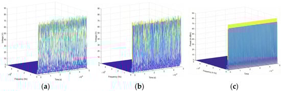
Figure 5. Time–frequency distribution of Duffing oscillator output signals under three different phase states: (a) chaotic state; (b) intermittent chaotic state; (c) large-scale periodic state.

(6) Phase point counting method on the circle [6]: A series of circular regions with equal-difference radii is drawn on the phase plane of the Duffing oscillator. The Duffing oscillator’s phase state can be judged by calculating the total number of phase points falling on the boundary of the circular area. This is a phase space feature with fast computation speed, making it highly suitable for engineering applications. However, it lacks a theoretical foundation and may not be accurate in complex situations.

3. Weak Signal Detection Model of Heterodyne Duffing Oscillators

According to the above analysis, except for the STFT method, most of the traditional chaotic phase state discrimination methods do not distinguish the intermittent chaotic state, which leads to a 0.03ω natural frequency detection error in the extended Duffing oscillator weak signal detection system. Therefore, a weak signal detection model based on the HDO is proposed in this paper. By introducing a new variable, the reference frequency ${\omega }_r$, to replace the original periodic internal driving force frequency $\omega$ for scale transformation of the Duffing equation, the expression of the different-frequency Duffing equation can be obtained as follows:

$$\ddot{x}+k{\omega }_r\dot{x}-{{\omega }_r}^{2}x+{{\omega }_r}^2{x}^3={{\omega }_r}^{2}F\cos (\omega t)$$

(8)

There are mainly two key parameters which would influence the equation characteristics compared with the original Holmes-type Duffing oscillator. The first one is ωr, which stands for the system’s reference frequency. And the second one is $\omega =R{\omega }_r$, which represents the periodic internal driving force’s frequency, where R is a positive integer. Therefore, for Equation (8), kωr stands for its damping coefficient, and the nonlinear part is still composed of x and x³ with coefficients related to ${\omega }_{r2}$. Last but not least, the right side of Equation (8) remains in the cosine form, while its amplitude and frequency are different from before. Just like the Holmes-type Duffing oscillator, which is composed of the damping part, the nonlinear part and the right-side driving force, the HDO also exhibits rich nonlinear dynamic characteristics. In this paper we set R = 2 for an analysis example; that is, ω = 2ωr. The bifurcation diagram of system (8) is shown in Figure 6.

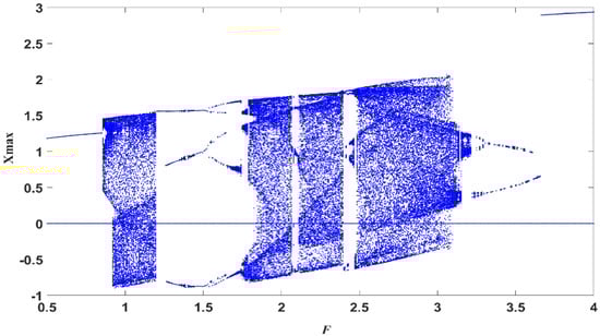
Figure 6. Bifurcation diagram of the HDO when R = 2.

We analyze the system properties using a bifurcation diagram. As shown in Figure 6, when $R=2$, the system exhibits rich dynamical behaviors and distinct phase transitions, which are sufficient to construct the detection criterion. An exhaustive analysis of the system dynamics for all possible $R$ values is a pure mathematical discussion that falls outside the scope of this paper, which focuses on the signal detection application. Therefore, in the revised manuscript, we have added a clarification stating that $R=2$ is chosen as a typical example to validate the method without loss of generality.

Figure 7 shows the phase plane trajectory and output time domain waveform of the HDO Equation (8) when it is in small- and large-scale periodic motion, respectively. When F ≤ F_c, the HDO will first transition to the vicinity of the outer orbit under the action of the internal driving force signal, and then transition back to the inner orbit due to insufficient driving force intensity. When F > F_c, driven by the internal dynamical signal, the HDO starts from the origin and finally makes a large-scale periodic motion on the outer orbit.

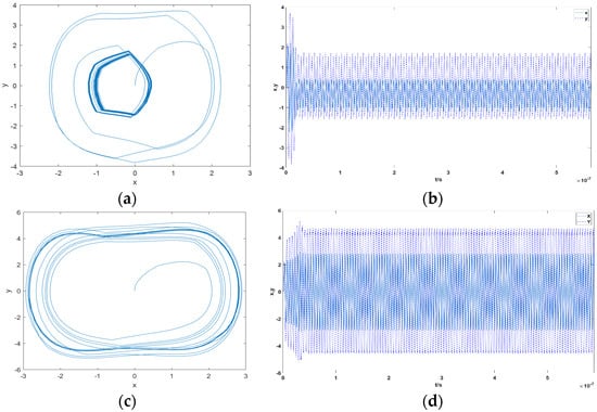
Figure 7. Output signals of HDO under different phase states: (a)$F=3.45$, phase plane trajectory; (b) $F=3.45,$ time domain waveform; (c) $F=3.54$, phase plane trajectory; (d) $F=3.54$, time domain waveform.

By substituting $\omega =2{\omega }_r$ into Equation (8), and then making $F=F_c$, and adding the weak periodic signal and noise to be measured to Equation (8), the damping term, nonlinear term, and internal driving force in Equation (9) become the same as those in Equation (8). The expression of the weak signal detection system based on the HDO can be obtained:

$$\ddot{x}+k{\omega }_r\dot{x}-{{\omega }_r}^{2}x+{{\omega }_r}^2{x}^3={{\omega }_r}^2\left(F_{\mathrm{c}}\cos (2{\omega }_{r}t)+A\cos ({\omega }_{0}t+{\phi }_0)+n(t)\right)$$

(9)

Here, $A\mathrm{c}\mathrm{o}\mathrm{s}\left({\omega }_{0}t+{\varphi }_0\right)$ represents the weak periodic signal to be detected, where $A$ and ${\varphi }_0$ denote its amplitude and initial phase, respectively, and $n\left(t\right)$ is the Gaussian white noise. The impact of these added components on the detection mechanism is visually demonstrated in Figure 8. As shown in Equation (9), the system is subjected to both the target signal and noise. In Figure 8a,b, when only the noise component $n\left(t\right)$ is present, its random nature fails to provide sufficient coherent energy to drive the system out of the critical state. Consequently, the phase trajectory remains confined within a small-scale chaotic attractor, demonstrating the system’s immunity to noise. In contrast, as shown in Figure 8c,d, the introduction of the specific periodic term $A\mathrm{c}\mathrm{o}\mathrm{s}\left({\omega }_{0}t+{\varphi }_0\right)$ acts as a resonant perturbation. Even with a weak amplitude, this coherent driving force disrupts the critical balance, triggering a phase transition from the small-cycle state to a large-scale periodic motion. This explicit transition confirms the feasibility of the proposed HDO system for weak signal detection.

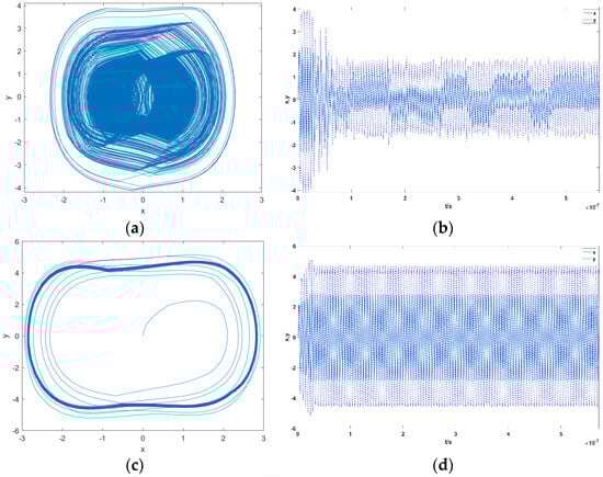
Figure 8. Output signal of small-cycle state HDO before and after inputting different signals: (a) input Gaussian white noise, phase plane trajectory; (b) input Gaussian white noise, time domain waveform; (c) input noisy target signal, phase plane trajectory; (d) input noisy target signal, time domain waveform.

In summary, the basic principle of using a HDO for weak signal detection is to take $F=F_c$, and set the system in a critical state. If a weak periodic signal with a specific frequency is added to the detection system, its state will transition from small periodic to large-scale periodic. Due to the significant difference between the phase trajectory and time sequence diagrams of the HDO in the small-cycle state and the large-scale periodic state, and the direct transition between the two states, there is no intermediate transition state. Therefore, even using the simplest amplitude judgment method can quickly and accurately distinguish the phase state of system (9) without generating detection errors caused by phase misjudgment.

4. Frequency Estimation Based on Heterodyne Duffing Oscillator

Due to the frequency difference between the internal driving force and the reference signal, when the input signal frequency ${\omega }_0$ is different, the HDO will exhibit different motion states. Table 1 shows the motion states of the proposed HDO under different periodic signal frequencies.

Table 1. Effect of input periodic signal frequency on the motion state of the Duffing oscillator.

Reference Frequency ${\mathit{f}}_{\mathit{r}}$/Hz	Input Cycle Signal Frequency Detection Ratio ${\mathit{f}}_0$/${\mathit{f}}_{\mathit{r}}$
	1	1.2	1.21	3	3.5	3.95	3.96	4
100 k	S	S	L	L	L	L	S	S
100 M	S	S	L	L	L	L	S	S
100 G	S	S	L	L	L	L	S	S

Note: The term “L” in the table refers to the large-scale periodic motion of the Duffing oscillator; “S” refers to the small periodic motion of the Duffing oscillator.

From Table 1, it can be seen that when the input periodic signal frequency ${\omega }_0$ is within $[1.21{\omega }_r,3.95{\omega }_r]$, the phase state of the multifrequency Duffing oscillator will change. To further determine ${\omega }_0$, the value of ${\omega }_0$ requires changing the reference frequency of the proposed detection system to intersect the frequency detection range of the two oscillators to a specific frequency value, ${\omega }_0$. However, for the HDO, when the reference frequency changes, its dynamic characteristics will also change accordingly. To ensure that the dynamic characteristics of the system are not affected, the input signal’s frequency can be controlled by setting a reference signal, and then setting the frequency to be estimated.

Therefore, the frequency estimation method based on the proposed HDO can be summarized as follows:

(1)

Construct a HDO for signal detection with reference frequency ${\omega }_r$; let $F=F_c$;

(2)

Mix and filter the measured signal with the reference signal, and then input it into the HDO signal detection system;

(3)

Adjust the reference signal’s frequency so that the HDO can realize the state transition from small periodic to large periodic and from large periodic to small periodic, respectively;

(4)

Record the frequency of the reference signal in the critical state of the system as ${\omega }_1$, ${\omega }_2$. Then, an estimate of the measured signal frequency ${\omega }_s$ can be obtained.

4.1. Frequency Resolution

To quantitatively study the frequency resolution of the HDO on periodic signals, we set the detection ratio thresholds of the HDO to be $c_1$ and $c_2$ respectively; that is, the HDOs all produce phase changes when the input signal frequency is ${\omega }_0\in$ [$c_1{\omega }_r$, $c_2{\omega }_r$]. At this point, the tested signal frequency ${\omega }_s$ meets $|{\omega }_1-{\omega }_s| = c_1{\omega }_r$ and $|{\omega }_2-{\omega }_s| = c_2{\omega }_r$.

In order to verify the effectiveness of our proposed method, the NRMSE of the frequency estimation accuracy is used for comparison between different typical methods under different signal-to-noise ratios, and the results are shown in Figure 9. The NRMSE (Normalized Root Mean Square Error) is defined as

$$\mathrm{NRMSE}={\displaystyle \frac{\sqrt{\frac{1}{N}{\displaystyle \sum _{k=1}^N{(x_k-x_0)}^2}}}{x_0}}$$

(10)

where $x_0$ stands for the true value of the parameter, $x_k$ is the parameter estimation, and $N$ is the estimated sequence length.

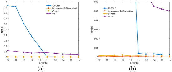
Figure 9. The frequency accuracy of the proposed method compared with the other literature and typical methods under different signal-to-noise ratios. (a) Overall performance. (b) Partial enlarged view.

Since ${\omega }_r$, ${\omega }_1$, and ${\omega }_2$ are all definite values, the frequency resolution $\Delta f$ is linearly dependent on the precision of the detection ratio $\delta c$ (where $\delta c=\left|\widehat{c}-c\right|$). The analytical expression is given by $\Delta f=\delta c\cdot f_r$, where $f_r={\omega }_r/2\pi$ represents the reference frequency of the Duffing oscillator system. This implies that the frequency resolution can be refined by increasing the precision of the critical threshold c₁ & c₂. Table 2 gives the simulation results of the critical frequency detection ratio threshold of HDO with different accuracies. During the experiment, the reference frequency of the detection system was fixed to $f_r=$100 MHz.

Table 2. Influence of the input periodic signals’ frequency on the motor state of the Duffing oscillator.

Critical Frequency Detection Ratio	Degree of Accuracy
	0.01	0.001	0.0001	0.00001	0.000001	0.0000001	0.00000001	0.000000001
c1	1.21	1.201	1.2001	1.20001	1.200001	1.2000001	1.20000001	1.200000001
c2	3.95	3.956	3.9567	3.95672	3.956720	3.9567207	3.95672076	3.956720766

While the frequency resolution $\Delta f$ is adjustable via the precision of the detection ratio $\delta c$, this adjustability comes with associated costs in computation time and hardware resources. The refinement of $\delta c$ relies on an iterative search process. As shown in Table 2, improving the resolution requires a smaller search step size, which directly increases the number of simulation cycles. In the proposed iterative architecture, the demand for logic resources does not scale significantly with resolution. To support a resolution of $\Delta f/f_r<{10}^{-6}$, a 64-bit double-precision unit is recommended.

From Table 2, the corresponding critical frequency detection ratio thresholds $c_1$, $c_2$ can be obtained at different accuracies, which can be selected according to the requirements of frequency resolution, and then adjusted for the reference signal frequency ${\omega }_1$, ${\omega }_2$, to meet the detection requirements. Compared with the frequency detection error of $0.03\omega$ of the weak signal detection method based on the extended-type Duffing oscillator, the signal detection method based on the HDO has adjustable frequency resolution, which greatly improves the frequency detection accuracy of the signal.

Figure 9 shows that the HDO method proposed in this paper has a significantly lower frequency estimation error NRMSE (−19 dB to −10 dB) compared to the other three methods. Especially when the signal-to-noise ratio is lower than −14 dB, the frequency estimation errors of other methods such as PCFCRD increase significantly, while the HDO method, due to its ability to adaptively adjust the frequency resolution, still maintains very low frequency estimation errors under low signal-to-noise ratios.

4.2. Real-Time Analysis

To further analyze the real-time performance of the weak signal detection method based on the HDO in this paper, we use an extended Duffing weak signal detection system and HDO weak signal detection system, and compare the time required for signal recognition with the same amount of data. Since the extended Duffing oscillators are prone to misjudgment when phase discrimination is made by the amplitude method, power spectroscopy and the STFT method are used, respectively, and the simulation results are shown in Figure 10.

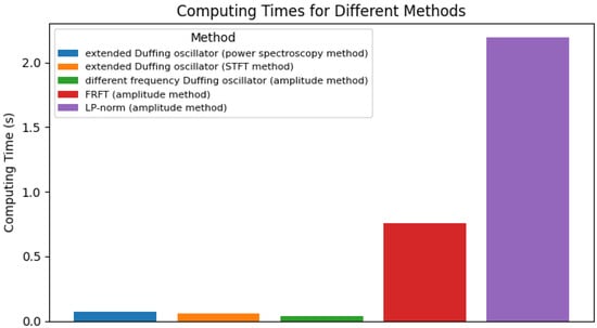
Figure 10. Computing times of the different methods.

The noise robustness and real-time performance are listed in Table 3. In the simulation, the signal length is set to 5 microseconds, the signal modulation period is 100 KHz, and the sampling frequency is 10 GHz. The computer CPU used for the simulation is an Intel Core i7 with a main frequency of 2.20 GHz and 16 GB of memory. As can be seen from Table 3 and Figure 10, the method presented in this paper demonstrates superior performance in terms of signal-to-noise ratio robustness and real-time capability. The proposed HDO method can complete the detection of weak signal parameters in just 0.038 s. Compared with other methods, even the STFT method, which is the fastest among the other methods, takes at least 0.058 s. This indicates that the phase state discrimination speed of the HDO method is at least 34.5% faster than those of other methods. The reason for this is that the HDO uses the amplitude judgment method to judge the phase state of the system, which improves the signal detection speed and can better meet the real-time requirements.

Table 3. Computing times of the different methods.

Method	Computing Time (s)	Computational Complexity	Noise Robustness (Min SNR)	Real-Time Performance
HDO	0.038	Low	<−25 dB	Excellent
Extended Duffing (STFT method)	0.058	Low	<−10 dB	High
Extended Duffing (power spectrum method)	0.069	Low	<−20 dB	High
FRFT	0.76	Medium	<−12 dB	Medium
PCFCRD	1.200	High	<−14 dB	Low
LP-norm	2.192	Very High	<−19 dB	Very Low

5. Parameter Estimation Method for Linear FM Sensor Signal

A continuous wave FM sensor sends a constant amplitude frequency-modulated continuous wave (FMCW) signal; the transmitted signal’s frequency will change according to the modulated signal. The linear FM sensor mainly includes two kinds: one is a triangular wave FM sensor, and the other is a sawtooth wave FM sensor. As one of the most widely used radio sensor systems on the battlefield, the FM sensor causes great difficulties with sensor interference due to its good anti-interception and anti-interference performance. In order to realize effective jamming of the LFM sensor, it is very important to intercept the sensor signal efficiently and estimate its working parameters accurately. Based on the correspondence between the input and output of the Duffing oscillator analyzed in the previous chapter, a signal parameter estimation method is proposed. Because of the high sensitivity to periodic or quasi-periodic signals and strong immunity to noise inherited from the typical Duffing oscillator, the proposed method is more suitable than other LFM signal parameter estimation methods, especially due to its great advantage in a low-SNR environment.

5.1. The Detection System’s Output Characteristics Excited by the Linear FM Sensor Signal

When excited by the linear FM sensor signal, if the influence of noise is ignored, the detection system can be expressed as

$$\left\{\begin{array}{l}\dot{x}=\omega y,\\ \dot{y}=\omega (-ky+x-x^3+F\cos (\omega t+\phi )+u(t)),\end{array}\right.$$

(11)

$u\left(t\right)$ acts as the input linear FM sensor signal, and the frequency at the initial time is the carrier frequency, that is, the central frequency $f_0$ of the signal. Taking the triangular wave-modulated linear FM sensor as an example, its instantaneous frequency can be expressed as

$$f\left(t\right)=\left\{\begin{array}{l}{f}_0+k_{f}t, n{T}_M-T_M/4<t\le n{T}_M+T_M/4\\ f_0-k_f\left(t-T_M/2\right), n{T}_M+T_M/4<t\le n{T}_M+3T_M/4\end{array}\right.$$

(12)

The starting frequency of the linear FM sensor signal f_start = f₀ − ΔFM/2 and the termination frequency f_end = f₀ + ΔFM/2 can be obtained.

At this time, the frequency difference is |Δω(t)| = |ω(t) − ω₀(t)| = 2π|f − (f₀ + k_f t)|. Because the LFM sensor signal’s frequency changes rapidly with time and the change range is usually greater than 0.03ω₀, it is difficult to directly measure its frequency using the phase transition from chaotic to large-scale periodic. For the linear FM sensor signal, its instantaneous frequency changes periodically with time, and the frequency difference between the internal power signals also changes periodically with time. Therefore, based on this kind of one-to-one correspondence between the frequency difference and the Duffing oscillator output signal obtained by analysis in Section 4, the modulation period can be estimated by the periodic variation characteristics of the linear FM sensor signal frequency.

The starting frequency of the linear FM sensor signal is ω_start = 2πf_start, and the termination frequency is ω_end = 2πf_end. According to the frequency relationship between the Duffing internal driving signal ω and the linear FM sensor signal, the following five cases, shown in Figure 11, are the corresponding Duffing oscillator outputs under different frequency relations. When fixed at k = 0.5, F_c = 0.8259, the internal signal frequency is changed: f = 75 MHz, 100 MHz, 125 MHz, 150 MHz, 175 MHz, respectively. In order to facilitate observation, the change in the temporal waveform of the Duffing oscillator output signal is clearer and intuitive. The input linear FM sensor signal’s amplitude is A = 1 V, and the other parameters are set to f_M = 100 kHz, f_start = 100 MHz, and f_end = 150 MHz.

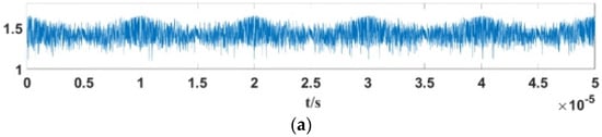
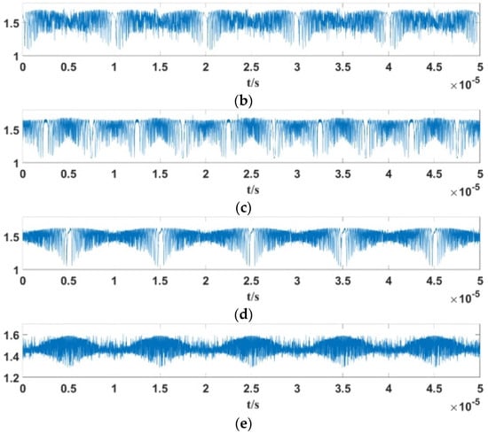
Figure 11. The corresponding Duffing oscillator output signal envelopes under different frequency relations: (a)$\omega <{\omega }_{start}$; (b) $\omega ={\omega }_{start}$; (c) ${\omega }_{start}<\omega <{\omega }_{end}$; (d) $\omega ={\omega }_{end}$; (e) $\omega >{\omega }_{end}$.

The following can be found from Figure 10: (1) When ω < ω_start or ω > ω_end, the linear FM sensor signal’s frequency varies between [ω_start, ω_end], while the Duffing oscillator’s internal policy power signal frequency ω is not in the frequency range of the linear FM sensor signal, which cannot meet the phase state jump conditions of the Duffing oscillator from chaotic to periodic. Thus, the system state is always chaotic. (2) When ω = ω_start or ω = ω_end, the Duffing oscillator’s internal signal frequency will equal that of the linear FM signal. Thus, there exists a period Δt such that the frequency difference |Δω| ≤ 0.03ω, at which point the system state will undergo large-scale periodicity. For the case of ω = ω_start, the periodic motion is present during every two modulation cycles, while for ω = ω_end, the periodic motion is present in the middle of each modulation cycle. (3) When ω_start < ω < ω_end, in each modulation cycle, with the increase and decrease in the linear modulation sensor signal frequency, the Duffing oscillator and linear modulation internal driving force signal frequencies appear twice in the alignment. Therefore, the modulation period estimation can be performed using the periodic variation in the system’s output signal.

By autocorrelation of the Duffing oscillator output signal, three results may occur, as shown in Figure 12.

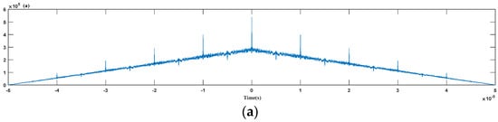
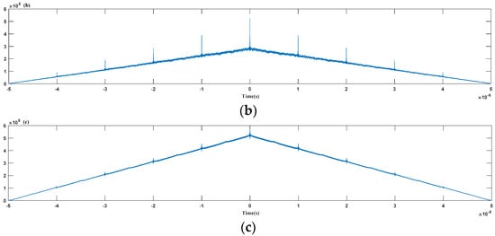
Figure 12. Autocorrelation function of the Duffing oscillator output signal in different cases: (a) half-periodic characteristic; (b) periodic characteristic; (c) non-periodic characteristic.

(1)

With carrier frequency ω₀ = (ω_start + ω_end)/2, when 0.9 ω₀ ≤ ω ≤ 1.1 ω₀, after the alignment, the autocorrelation function has a half-periodic characteristic; i.e., the average of two adjacent local maxima is about 0.5 times the modulation period, which can be seen in Figure 12a. When the input signal amplitude decreases, the half-periodic characteristic disappears quickly, as shown in Figure 12b. Furthermore, the periodic characteristics gradually disappear as the signal-to-noise ratio decreases, as shown in Figure 12c.

(2)

When ω_start ≤ ω < 0.9 ω₀ or 1.1 ω₀ < ω ≤ ω_end, the signal shows good periodic characteristics, and the average of the two local maxima adjacent to the autocorrelation function is equal to the modulation period as shown in Figure 12b. With the decreasing signal-to-noise ratio, the periodic characteristics disappear, as shown in Figure 12c.

(3)

When ω < ω_start or ω > ω_end, although the oscillator state always remains chaotic, the relationship between the amplitude of the system output and the frequency difference remains unchanged, decreasing with the increase in the difference frequency, and the confusion of the system still exhibits a periodic change characteristic. The modulation period after treatment using self-correlation is clearly shown in Figure 12b. But we should know that this periodic characteristic shows great correlation with the input signal’s amplitude; if the input signal amplitude is too weak, the periodic characteristics will no longer exist, and if the signal-to-noise ratio decreases, the periodic characteristics will gradually disappear, as shown in Figure 12c.

According to the definition of the autocorrelation function, for the periodic characteristic, the position of the local maximum point of the autocorrelation function corresponds to a case of signal delay in a modulation period, while for the half-periodic characteristic, the position of the local maximum point of the autocorrelation function corresponds to the half-modulation period of signal delay. The frequency change in the half-modulation cycle of the triangular wave is different, and the frequency difference change in the internal power signal is also different. In addition, the size of the difference frequency and the positive and negative values will affect the oscillator’s output signal. Therefore, when the signal’s self-correlation is sought, if only half is delayed rather than the whole modulation period, then the difference frequency of the oscillator’s output signal is not completely different, except when the difference frequency of the output signal is zero, in which case the oscillator’s output signal is also different. Therefore, only when the system’s internal power signal frequency is exactly equal to the carrier frequency or is located in a small frequency range, when 0.9ω₀ ≤ ω ≤ 1.1ω₀, the change in the relative amplitude of the calculated autocorrelation function will be significantly smaller than the signal delay for a complete modulation period. The period and half-period properties can therefore be distinguished by the relative amplitude magnitude of the local maximum point of the autocorrelation.

5.2. Parameter Estimation of Linear FM Sensor Signal by Duffing Oscillator and Frequency Periodicity

Constructed from the frequency periodicity obtained by the analysis in Section 5.1, the modulation period of the linear FM sensor signal can then be determined by the autocorrelation function of the oscillator’s output signal. Because the half-cycle characteristic of the output signal autocorrelation function has high requirements on the amplitude strength of the input linear FM sensor signal, it cannot fully cover the linear FM sensor signal’s frequency range, resulting in large restrictions. Therefore, here in this paper, we primarily use the parameter estimation of the weak linear FM sensor signal by analyzing the oscillator’s output signal autocorrelation feature; i.e., the signal modulation period T_M is obtained by averaging adjacent local maxima of the autocorrelation.

Combined with the analysis in Section 5.1, when the frequency of the oscillator’s driving force signal is in the range of the linear FM sensor signal’s frequency, that is, ω_start ≤ ω ≤ ω_end, in each modulation period, the signal has a period Δt; i.e., the frequency difference |Δω| ≤ 0.03ω, and the oscillator makes a periodic motion. In general, the power spectrum feature of chaotic signals shows that they have widely and continuously distributed small peaks, while the power spectrum feature of periodic signals shows that they tend to contain fewer peaks than the chaotic state; the latter is a more concentrated distribution with higher peaks. From these analyses, we can obtain that the state of the signal can be determined by power spectroscopy. We can divide the output signal into several finite-length signals and then calculate the maximum estimation of the power spectrum for each finite-length signal. The power spectrum estimate must satisfy a quantitative criterion. Specifically, we adopt an adaptive threshold strategy based on the 3 dB principle. First, the global maximum power spectrum value $P_{max}$ among all finite-length signals is identified. The detection threshold $P_{th}$ is then defined as 3 dB lower than $P_{max}$. If the power spectrum estimate of a signal segment exceeds $P_{th}$, it is determined to be in a periodic state; otherwise, it is classified as in a chaotic or transition state. Of course, larger peaks may also occur, but they are usually irregular, not only with peaks much smaller than the periodic signal, but possibly at any location in the modulation cycle. Therefore, the secondary discrimination of chaotic and periodic states by estimating the maximum value of the power spectrum interval can effectively reduce the probability of miscalculation.

When ω_start ≤ ω ≤ ω_end, the linear FM sensor signal of the triangular wave and sawtooth wave is used as the oscillation system’s input in different frequency relations. Figure 12 and Figure 13 are the plots of the maximum estimation of the system output’s power spectral density function over time. Specifically, the modulation signal has a modulation frequency of f_M = 100 kHz, and the modulated sensor signal is f_start = 100 MHz, f_end = 150 MHz, A = 1 V. The basic parameters of the Duffing oscillator signal detection system were set to k = 0.5, F_c = 0.8259, and the internal power signal frequency was f = 100 MHz, 125 MHz, and 150 MHz.

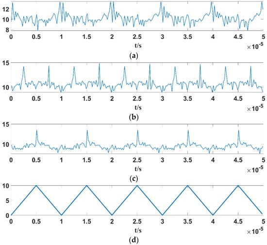
Figure 13. Variation curves of the maximum value of the power spectral density function of the Duffing oscillator output signal with different conditions: (a) triangular wave linear frequency modulation sensor signal, ω = ω_start; (b) triangular wave linear frequency modulation sensor signal, ω_start < ω < ω_end; (c) triangular wave linear frequency modulation sensor signal, ω = ω_end; (d) time domain waveform of the triangle wave linear modulation sensor signal.

By comparing the maximum time-varying curve of the oscillator’s output signal’s power spectral density function with the original waveform, the following is obtained:

(1)

If ω = ω_start, for the triangular wave linear FM sensor signal excitation, the periodically maximum power spectrum estimate will appear between two adjacent modulation cycles, as shown in Figure 13a. But for sawtooth wave linear FM sensor signal excitation, the periodically maximum power spectrum estimate will appear at the beginning point of each modulation cycle, as shown in Figure 14a.

Figure 14. Variation curves of the maximum value of the power spectral density function of the Duffing oscillator output signal with different conditions: (a) sawtooth wave linear frequency modulation sensor signal, ω = ω_start; (b) sawtooth wave linear frequency modulation sensor signal, ω_start < ω < ω_end; (c) sawtooth wave linear frequency modulation sensor signal, ω = ω_end; (d) time domain waveform of the sawtooth wave linear modulation sensor signal.

(2)

If ω = ω_end, for the triangular wave linear FM sensor signal excitation Duffing output signal, the periodically maximum power spectrum estimation will appear in the middle of each modulation cycle, as shown in Figure 13c. But for sawtooth wave linear FM sensor signal excitation, the periodically maximum power spectrum estimation is generated at the end position of each modulation cycle, as shown in Figure 14c.

(3)

If ω_start < ω < ω_end, whether the oscillator is excited by either a triangular wave or zigzag wave, the periodically maximum power spectrum will appear between the positions described in (1) and (2), and the specific position is related to the relative position of ω in the [ω_start, ω_end] interval. In particular, in the case of triangular wave linear FM sensor signal excitation, two local maximum power spectrum estimates appear in each modulation period, and the periodically maximum power spectrum estimate may appear in either of them, as shown in Figure 13b and Figure 14b.

The core idea of Figure 13 and Figure 14 lies in whether the internal frequency is equal to the frequency to be measured. Since equality in frequency will cause a phase transition, if we divide the output signal into several finite-length signals and use the power spectrum method to determine the maximum power spectrum value of each finite-length signal, then in the curve diagram of the maximum estimated value of the power spectrum density function of the output signal as a function of time, a peak will form at the location where the frequencies are equal, corresponding to the modulation method of the signal to be measured.

Therefore, through the position and interval of the estimated maximum power spectrum of the oscillator’s output signal period, the oscillator aligned with the frequency of the linear FM sensor signal can be found, the start and stop frequencies of the linear FM sensor signal are determined, and the linear FM sensor signal parameter estimation is completed.

In conclusion, a parameter estimation method for linear FM sensor signals based on the frequency periodicity of Duffing oscillators under low-SNR scenarios is summarized as follows:

(1)

Set different internal driving signal frequencies for the oscillator array, and make F = F_c.

(2)

Take the weak linear frequency modulation sensor signal to be tested as a system input, conduct autocorrelation with the output signal x(t) of each oscillator, and take the envelope to obtain Rx(t).

(3)

Find the autocorrelation Rx(t)’s local maximum point. If the local maximum points’ total number is more than one, the internal policy dynamic signal frequency of the oscillator is considered to meet ω_start ≤ ω ≤ ω_end. The linear FM sensor signal’s modulation period T_M can be estimated from intervals of adjacent local maximum points.

(4)

The maximum estimate of the power spectral density function P_max(t) is obtained after dividing the Duffing oscillator output signal x(t).

(5)

Match the local maximum point of autocorrelation Rx(t) to P_max(t) to obtain the monotonous periodic T_M of P_maxj(t).

(6)

Find the maximum value of P_j and the positions of each P_maxj(t). If the adjacent P_j interval equals the modulation period T_M, the oscillator’s internal driving signal frequency is considered to meet ω_start ≤ ω ≤ ω_end.

(7)

Combine the results of steps 3 and 6. Comprehensively judge the Duffing oscillator for all frequency alignments. The location of P_j with the smallest frequency of the internal signal is used as the modulation period starting point.

(8)

Further determine the maximum value position of P_maxj(t) of the oscillator aligned with the remaining frequencies. If the start and stop frequency determination conditions are satisfied, the linear frequency modulation sensor signal’s carrier frequency (center frequency), frequency deviation, and frequency modulation slope can be obtained, thus completing the signal parameter estimation. On the contrary, the internal driving signal frequency of the Duffing oscillator array should be adjusted according to the result of step 7 and the method should be re-executed starting back at step 1.

The specific processing flow is plotted in Figure 15.

Figure 15. Flowchart of parameter estimation of linear FM sensor signal by Duffing oscillator based on frequency periodicity under low SNRs.

5.3. Simulation Analysis of the Linear FM-Induced Signal Parameter Estimation Algorithm Under Different SNRs

An oscillator array consisting of five Duffing oscillators with different internal force signal frequencies is constructed, and the internal force signal’s initial frequencies are set to f = 75 MHz, 100 MHz, 125 MHz, 150 MHz, and 175 MHz, respectively. The to-be-estimated LFM sensor signal’s working parameters are set as follows: A = 0.05 V kHz, f_M = 100 V, f₀ =125 MHz, the triangular wave’s frequency modulation slope k_f = 10⁴ GHz·s⁻¹, and k_f = 5000 GHz·s⁻¹ for the sawtooth wave. In all, the sampling frequency f_s = 10 GHz.

In the experiment, adjusting the noise intensity was used to get the lowest detection threshold of the input signal-to-noise ratio. When amplitude A is 0.05 V, the signal-to-noise ratios corresponding to 0 dB, −10 dB, −20 dB, −25 dB, −26 dB, and −27 dB can be obtained by taking the noise intensity values σ² = 0.00125, 0.0125, 0.125, 0.395, 0.5, and 0.6265, respectively. Simulation experiments were conducted under different SNRs according to the steps in Section 5.2. The estimation results for linear FM sensor signal parameters can be seen in Table 4.

Table 4. Simulation of the LFM sensor signal parameter estimation results under different SNRs. Adapted from Ref. [6].

SNR/dB	Triangular Wave					Sawtooth Wave
	TM/μs	fM/kHz	f0/MHz	kf		TM/μs	fM/kHz	f0/MHz	kf
				GHz·s−1	Relative Error/%				GHz·s−1	Relative Error/%
−10	9.9999	100	125	10,000	0	10.001	99.99	125	4999.60	0.008
−15	9.9999	100	125	10,000	0	10.0005	100	125	4999.90	0.005
−20	9.9999	100	125	10,000	0	9.9999	100	125	5000.10	0.002
−23	9.9988	100.01	125	10,001.20	0.012	9.9999	100	125	5000.10	0.002
−25	9.998	100.02	125	10,002	0.02	9.9999	100	125	5000.10	0.002
−27	9.69	103.2	None	None	None	9.6466	103.66	None	None	None

The experimental results show that the parameter estimation method of the Duffing oscillator LFM sensor based on frequency periodicity proposed here can obtain effective estimation of the carrier frequency, modulation frequency, and FM slope of LFM sensor signals under different signal-to-noise ratios, and the lowest detection threshold of the input signal-to-noise ratio can reach −25 dB, and some parameter estimations may fail at −26 dB or even lower SNRs. Future work will further study how to effectively solve the problem when the signal-to-noise ratio is even lower. Taking the triangular wave LFM sensor signal as a comparison, the sawtooth LFM sensor signal contains an abrupt change from the cutoff frequency to the starting frequency between two adjacent modulation periods, which leads to a rapid change in the oscillator’s motion state in a very short time. At this time, there may be a large error in the sawtooth LFM sensor signal frequency estimation if the power spectrum method is still used to distinguish the oscillator’s motion state. Due to the fact that this method uses the estimated value of the average power spectrum over time as the basis for judgment, when the time is not selected properly, even when including the periodic motion and chaotic motion of the oscillator, the estimated value of the power spectrum after reaching the average may be much lower than those of other periods; the estimated frequency could then produce a large error, or even be difficult to measure. Therefore, the triangular LFM sensor signal’s parameter estimation performance is better than that of the sawtooth type. As can be seen from Table 4, although the detection accuracy of the triangular wave LFM sensor signal decreases under the environment of −26 dB, the relative error of its FM slope estimation is as small as 0.168%; thus, it still obtains high-precision estimation results.

To further clarify the applicable range of the proposed method, we evaluated the estimation performance under different LFM parameters. Figure 16a shows the impact of the frequency modulation slope; the relative error exhibits a slight upward trend but remains consistently below 0.5%. This indicates that while extremely fast modulation slopes may slightly reduce the interaction time between the signal and the oscillator, the method maintains high accuracy within a practical range. Figure 16b depicts the error curve with respect to the signal bandwidth. The estimation error remains stable and less than 0.4%, demonstrating that the method effectively adapts to different bandwidth configurations. These results verify that the proposed HDO-based method is robust not only to noise but also to variations in signal parameters.

Figure 16. The estimation error curves for varying modulation slopes and bandwidths at an SNR of −20 dB. (a) The impact of the frequency modulation slope; (b) the impact of the signal bandwidth.

To strictly evaluate the proposed method, we compared the HDO with the traditional extended Duffing oscillator which relies on intermittent chaos. The results are shown in Table 5.

Table 5. Comprehensive comparison between traditional Duffing methods and the proposed HDO in the intermittent chaos state.

	Extended Duffing	HDO
Threshold Stability	Sensitive: the boundary between intermittent chaos and pure chaos is fuzzy and sensitive to noise variance.	Stable: the transition is a sharp binary jump; the critical threshold is adaptively adjusted.
Frequency Detection Range	Narrow: requires strict frequency matching, ω ≈ ω0.	Adjustable: utilizes the heterodyne principle, and can be flexibly covered across different frequency bands by adjusting ωr.
Computing Time	Slow, 0.058 s for STFT.	Fast, 0.038 s, real-time performance improved by >34.5%.

To further validate the stability and efficiency of the proposed method, we analyzed the algorithm’s numerical convergence regarding iteration counts and initial condition sensitivity. Unlike traditional iterative optimization algorithms that may require hundreds of iterations, our method employs a “Coarse-to-Fine” strategy. The oscillator array provides an initial coarse frequency range, and the power spectrum estimation directly locates the dominant frequency component. Simulation results indicate that the frequency estimation loop typically converges within two to three iterations, as shown in Figure 17a, which can also explain the high real-time performance reported in Table 3. For sensitivity to initial conditions, we tested the detection performance under randomized initial values $\left(x_0,{\dot{x}}_0\right)$. The results demonstrate that while the chaotic state is sensitive to initial values, as shown in Figure 17b the target large-scale periodic state acts as a stable global attractor. Therefore, the phase state discrimination result is robust to initial conditions within a wide range, ensuring reliable detection in practical engineering.

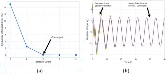
Figure 17. The algorithm’s numerical convergence regarding iteration counts and its sensitivity to the oscillator’s initial conditions. (a) Iteration counts; (b) initial condition sensitivity.

6. Conclusions

This article studies weak signal detection and parameter estimation methods applicable to millimeter-wave signals. At present, the detection and parameter estimation methods for weak signals in Duffing oscillators based on critical thresholds have difficulty bypassing intermittent chaotic states, which requires accurate determination of which segments are periodic and which are chaotic in the output timing, and requires high accuracy in phase discrimination. However, existing chaotic phase discrimination methods often use the average motion state of the system over a period of time to determine the phase state, which easily confuses intermittent chaotic states with periodic states, directly leading to low accuracy and efficiency in phase discrimination and critical threshold determination in existing chaotic phase discrimination methods. To this end, this article proposes a weak signal detection model for the Duffing oscillator with different frequencies. The proposed system can avoid intermittent chaotic states, making the phase discrimination of the system simpler, faster, and more accurate. At the same time, not only can the parameter settings be adjusted according to the need to adapt to different frequency resolutions, but the real-time performance is also significantly better than that of methods based on traditional Duffing equations.

In the future, we will consider two aspects. Firstly, we will further develop the performance of the cross-frequency Duffing oscillator to enable it to estimate more signal parameters, including modulation frequency, center frequency, and bandwidth. Secondly, future work will concentrate on the implementation of the HDO algorithm on an FPGA-based hardware platform and verify its effectiveness in real-world millimeter-wave sensor detection scenarios to further complement the theoretical results presented here.

References

- Yang, B.; Guo, Z.; Wu, K.; Huang, Z. Study of Millimeter-Wave Sensor Echo Characteristics under Rainfall Conditions Using the Monte Carlo Method. Appl. Sci. 2024, 14, 8352. [Google Scholar] [CrossRef]
- Shastri, A.; Valecha, N.; Bashirov, E.; Tataria, H.; Lentmaier, M.; Tufvesson, F.; Rossi, M.; Casari, P. A review of millimeter wave device-based localization and device-free sensing technologies and applications. IEEE Commun. Surv. Tutor. 2022, 24, 1708–1749. [Google Scholar] [CrossRef]
- Birx, D.L.; Pipenberg, S.J. Chaotic oscillators and complex mapping feed forward networks (CMFFNS) for signal detection in noisy environments. In Proceedings of the IJCNN International Joint Conference on Neural Networks, Baltimore, MD, USA, 7–11 June 1992; IEEE: Piscataway, NJ, USA, 1992; pp. 881–888. [Google Scholar]
- Wang, G.Y.; Chen, D.J.; Lin, J.Y.; Chen, X. The Application of Chaotic Oscillators to Weak Signal Detection. IEEE Trans. Ind. Electron. 1999, 46, 440–444. [Google Scholar] [CrossRef]
- Wang, G.Y.; He, S.L. A quantitative study on detection and estimation of weak signals by using chaotic Duffing oscillators. IEEE Trans. Circuits Syst. Fundam. Theory Appl. 2003, 50, 945–953. [Google Scholar] [CrossRef]
- Zhang, N.; Yan, X.; Lv, M.; Chen, X.; Huang, D. Parameter estimation method for a linear frequency modulation signal with a Duffing oscillator based on frequency periodicity. Chin. Phys. B 2023, 32, 080701–080711. [Google Scholar] [CrossRef]
- Yuan, Y.; Li, Y.; Mandic, D.P.; Bao-Jun, Y. Regular nonlinear response of the driven Duffing oscillator to chaotic time series. Chin. Phys. B 2009, 18, 958–968. [Google Scholar] [CrossRef]
- Hou, J.; Yan, X.P.; Li, P.; Hao, X.-H. Weak wide-band signal detection method based on small-scale periodic state of Duffing oscillator. Chin. Phys. B 2018, 27, 209–219. [Google Scholar] [CrossRef]
- Cheng, M.F.; Zhang, W.W.; Wu, J.; Ma, H. Analysis and application of weak guided wave signal detection based on double Duffing oscillators. Mech. Syst. Signal Process. 2023, 191, 110196. [Google Scholar] [CrossRef]
- Dou, Y.; Li, S.; Lin, B. The parameter estimation of LFM signal using the generalized Versoria Wigner-Ville distribution in impulsive noise. In Proceedings of the 2023 IEEE/CIC International Conference on Communications in China (ICCC), Dalian, China, 10–12 August 2023; IEEE: Piscataway, NJ, USA, 2023; pp. 1–6. [Google Scholar]
- Li, W.; Xiong, Y.; Wei, C.; Chen, P.; Liang, D.; Peng, Z. Near-field micro-Doppler effect and spectrum characteristics of rotating targets: Theoretical analysis and parameter estimation method. IEEE Trans. Instrum. Meas. 2023, 72, 8006212. [Google Scholar] [CrossRef]
- Cai, J.-H.; Xiao, Y.-L.; Fu, L.-Y. Fault diagnosis of rolling bearing based on fractional Fourier instantaneous spectrum. Exp. Tech. 2022, 46, 249–256. [Google Scholar] [CrossRef]
- Xu, F.; Bao, Q.; Chen, Z.; Pan, S.; Lin, C. Parameter Estimation of Multi-Component LFM Signals Based on STFT Hough Transform and Fractional Fourier Transform. In Proceedings of the 2018 2nd IEEE Advanced Information Management, Communications, Electronic and Automation Control Conference (IMCEC), Xi’an, China, 25–27 May 2018; IEEE: Piscataway, NJ, USA, 2018; pp. 839–842. [Google Scholar]
- Zheng, J.; Liu, H.; Liu, Q.H. Parameterized Centroid Frequency-Chirp Rate Distribution for LFM Signal Analysis and Mechanisms of Constant Delay Introduction. IEEE Trans. Signal Process. 2017, 65, 6435–6447. [Google Scholar] [CrossRef]
- Koç, E.; Koç, A. Fractional Fourier transform in time series prediction. IEEE Signal Process. Lett. 2022, 29, 2542–2546. [Google Scholar] [CrossRef]
- Şahinuç, F.; Koç, A. Fractional Fourier transform meets transformer encoder. IEEE Signal Process. Lett. 2022, 29, 2258–2262. [Google Scholar] [CrossRef]
- Alikaşifoğlu, T.; Kartal, B.; Koç, A. Graph fractional Fourier transform: A unified theory. IEEE Trans. Signal Process. 2024, 72, 1325–1336. [Google Scholar] [CrossRef]
- Chen, X.; Guan, J.; Bao, Z.; He, Y. Detection and extraction of target with micromotion in spiky sea clutter via short-time fractional fourier transform. IEEE Trans. Geosci. Remote Sens. 2014, 52, 1002–1018. [Google Scholar] [CrossRef]
- Yang, Y.; Peng, Z.; Zhang, W.; Meng, G. Parameterized time-frequency analysis methods and their engineering applications: A review of recent advances. Mech. Syst. Signal Process. 2019, 119, 182–221. [Google Scholar] [CrossRef]
- Zhao, D.; Wang, H.; Cui, L. Frequency-chirp-rate synchrosqueezing-based scaling chirplet transform for wind turbine nonstationary fault feature time–frequency representation. Mech. Syst. Signal Process. 2024, 209, 111–122. [Google Scholar] [CrossRef]
- Guan, Y.; Feng, Z. Adaptive linear chirplet transform for analyzing signals with crossing frequency trajectories. IEEE Trans. Ind. Electron. 2021, 69, 8396–8410. [Google Scholar] [CrossRef]
- Hatano, N.; Kawasumi, R.; Sawano, Y. Sparse non-smooth atomic decomposition of quasi-Banach lattices. J. Fourier Anal. Appl. 2022, 28, 61–74. [Google Scholar] [CrossRef]
- Wang, W.; Yan, S.; Mao, L.; Sui, Z.; Yang, J. Ambiguity-Free Broadband DOA Estimation Relying on Parameterized Time-Frequency Transform. IEEE Signal Process. Lett. 2025, 32, 1211–1215. [Google Scholar] [CrossRef]
- Chen, L.; Wang, Z.; Xu, L. A general parameterized time-frequency analysis based on multiple squeezing mechanism. In Proceedings of the 2023 6th International Conference on Information Communication and Signal Processing (ICICSP), Xi’an, China, 23–25 September 2023; IEEE: Piscataway, NJ, USA, 2023; pp. 348–352. [Google Scholar]
- Hu, Z.; Ma, H. Blind modal estimation using smoothed pseudo Wigner–Ville distribution and density peaks clustering. Meas. Sci. Technol. 2020, 31, 105004–105013. [Google Scholar] [CrossRef]
- Li, X.; Sun, Z.; Zhang, T.; Yi, W.; Cui, G.; Kong, L. WRFRFT-based coherent detection and parameter estimation of radar moving target with unknown entry/departure time. Signal Process. 2022, 166, 107228. [Google Scholar] [CrossRef]
- Barkat, B.; Boashash, B. Instantaneous frequency estimation of polynomial FM signals using the peak of the PWVD: Statistical performance in the presence of additive gaussian noise. IEEE Trans. Signal Process. 2002, 47, 2480–2490. [Google Scholar] [CrossRef]
- Akilli, M.; Yilmaz, N. Study of weak periodic signals in the EEG signals and their relationship with postsynaptic potentials. IEEE Trans. Neural Syst. Rehabil. Eng. 2018, 26, 1918–1925. [Google Scholar] [CrossRef] [PubMed]
- Zhang, K.; Xu, G.; Du, C.; Wu, Y.; Zheng, X.; Zhang, S.; Han, C.; Liang, R.; Chen, R. Weak feature extraction and strong noise suppression for SSVEP-EEG based on chaotic detection technology. IEEE Trans. Neural Syst. Rehabil. Eng. 2021, 29, 862–871. [Google Scholar] [CrossRef]
Disclaimer/Publisher’s Note: The statements, opinions and data contained in all publications are solely those of the individual author(s) and contributor(s) and not of MDPI and/or the editor(s). MDPI and/or the editor(s) disclaim responsibility for any injury to people or property resulting from any ideas, methods, instructions or products referred to in the content. |
© 2026 by the authors. Licensee MDPI, Basel, Switzerland. This article is an open access article distributed under the terms and conditions of the Creative Commons Attribution (CC BY) license.