


Abstract
This work proposes a novel autoregressive (AR) modeling framework in which the model structure and coefficients are induced from the analytical properties of Butterworth filters. By exploiting the equivalence between AR models and all-pole discrete-time filters, the proposed approach derives the AR coefficients directly from the pole locations of a continuous-time Butterworth prototype mapped to the discrete-time domain. In this formulation, the filter order and stopband attenuation act as hyperparameters controlling the complexity and frequency-selective behavior of the resulting predictor, while a scalar gain parameter is estimated from data using a maximum likelihood criterion. Model selection is carried out through a nested cross-validation strategy tailored to time series data, employing a rolling-origin scheme to prevent look-ahead bias. The predictive performance of the resulting Butterworth-induced AR models is evaluated using one-step-ahead forecasts and compared against classical ARIMA models on simulated data. Experimental results show that the proposed approach achieves competitive predictive accuracy, while offering a structured and interpretable link between frequency-domain filter design and time-domain autoregressive modeling.
Keywords:
autoregressive model; Butterworth filter; matched Z-transform all-pole filter; filter order MSC:
62M10; 62M15; 62M20
1. Introduction
Autoregressive (AR) processes are a fundamental class of discrete-time stochastic models widely applied in econometrics, control theory, and signal analysis, see for example [1]. This type of process can be rigorously interpreted as a linear time-invariant (LTI) system, providing a unified mathematical framework for analyzing its structure, stability, and spectral properties, see [2,3]. Formally, an AR process of order p, denoted by AR(p), is defined by the recursive relation,
where are the real-valued coefficients of the model, and is a white noise sequence with zero mean and variance . In this work, the process is assumed to be mean-centered, so that the intercept term is zero. In this formulation, the process can be interpreted as consisting of two components: a deterministic part, given by the linear combination of past values , responsible for predicting the current sample from its history, and a stochastic part, given by , which represents the innovation or unpredictable component of the signal.
The AR coefficients are typically estimated from observed data using standard statistical methods. The Yule–Walker equations exploit the autocorrelation structure of the process to analytically solve for the coefficients, see [1]. The method of moments relies on matching theoretical moments with their sample counterparts, such as autocovariances, to estimate the model parameters, see [4]. Alternatively, least-squares estimation determines the coefficients by minimizing the sum of squared prediction errors over the observed data, see [5]. All these approaches aim to capture the linear dependence of the current observation on past values, thereby identifying the deterministic predictive structure embedded in the stochastic process.
Recent large-scale surveys and comparative studies show that the current state of the art in time series forecasting is largely driven by hybrid and deep learning–based approaches, which combine traditional statistical models with machine learning architectures to maximize predictive accuracy, often at the expense of model interpretability, see [6,7,8]. This trend has led to highly accurate yet largely opaque forecasting systems, limiting their usefulness in applications where understanding the underlying dynamics is as important as prediction accuracy. In contrast to this prevailing black-box paradigm, the present work seeks to exploit the intrinsic structural properties of autoregressive processes. Unlike conventional autoregressive modeling, in which the coefficients are directly estimated from data, and unlike frequency-domain constrained AR methods such as maximum entropy or Burg spectral estimation, which determine the AR coefficients by fitting a spectrum that maximizes entropy or minimizes forward and backward prediction errors under spectral constraints, the proposed framework analytically specifies a Butterworth spectral prototype and induces the corresponding autoregressive coefficients from its pole distribution.
From a broader perspective, existing time series forecasting approaches can be roughly grouped into three classes: data-driven autoregressive models, spectral fitting methods, and black-box machine learning models. Data-driven AR and ARIMA models estimate coefficients directly from finite and noisy data, which often leads to unstable pole locations, spurious spectral peaks, and limited physical interpretability, see [9,10]. Spectral fitting methods such as maximum entropy or Burg estimation impose a desired spectral profile indirectly through optimization, but the resulting pole configurations are highly sensitive to noise and model order and remain difficult to interpret in terms of system dynamics, see for example [3,10]. Modern deep learning and hybrid approaches further maximize predictive accuracy at the cost of transparency and physical meaning, see [11]. These limitations highlight the absence of a principled autoregressive modeling framework that allows the spectral structure to be prescribed analytically, while simultaneously ensuring stability, smooth spectral behavior, and physical interpretability of the resulting model. Thus, the aim of this work is to develop a filter-based methodology for constructing autoregressive models by inducing their coefficients from the poles of a Butterworth filter, thereby combining analytical spectral control with the interpretability of all-pole AR representations.
The proposed Butterworth-induced AR model (BTW-AR) addresses a structural limitation shared by all these approaches: none provides a principled way to prescribe, in closed form, a smooth, stable, and physically interpretable spectral envelope while retaining the parsimonious all-pole structure of an AR model. By specifying a Butterworth prototype, the desired low-pass spectral shape is analytically fixed through its maximally flat magnitude response and monotonic roll-off, see [2,12], and the corresponding autoregressive representation is induced directly from the resulting pole distribution. This yields AR models whose spectral properties, stability, and dominant time constants are controlled a priori, rather than being inferred from noisy data or opaque optimization procedures, see [13].
The BTW–AR model is particularly well suited for applications involving band-limited feedback systems, in which accurate prediction must be achieved without sacrificing the interpretability of the underlying dynamics. Typical examples include physiological control mechanisms such as heart rate and blood pressure regulation, see [14,15,16], as well as mechanical and thermal control systems, and low-frequency economic or environmental processes. In these contexts, the poles of the induced AR model admit a direct physical interpretation in terms of dominant time constants, see [17], damping, and stability properties, an interpretation that is generally unavailable in purely data-driven or black-box forecasting approaches, see [18]. Motivated by this observation, the proposed framework determines both the autoregressive coefficients and the model order p by exploiting the structural equivalence between autoregressive models and all-pole filter representations. Rather than estimating the AR parameters directly from the data, they are induced from the pole locations of a Butterworth low-pass filter, whose poles are optimally distributed to produce a maximally flat magnitude response.
This approach contrasts with the classical direction, in which a spectral representation is constructed from an estimated autoregressive (AR) model, see [5,19]. Instead, it exploits the well-defined analytical structure of the Butterworth frequency response to guide the selection of the model order p and to induce the corresponding autoregressive coefficients.
It is worth noting that the relationship between autoregressive models and analog filter prototypes has been explored in previous studies. Early work has shown that AR spectra can be interpreted or approximated using classical all-pole filter families, including Butterworth structures, see for example [9,20]. Moreover, Butterworth filters and related analog prototypes have been employed in some studies as preprocessing stages prior to conventional AR parameter estimation or spectral analysis, see [19,21]. These contributions, however, primarily focus on spectral interpretation or preprocessing, whereas the present work leverages the analytical properties of the Butterworth filter to directly induce the structure and parameters of the AR model.
The structure of this paper is as follows. Section 2 will be devoted to the study of a direct relationship between the recursive structure of the autoregressive models of order p and the convolution representation as causal linear time-invariant (LTI) systems. The approach of infinite impulse response filters and design based on the Butterworth approximation is presented in Section 3. In particular, a Butterworth filter approximation is explored, considering some specific characteristics and properties. The matched Z-transform process is employed to directly map each analogue pole to a corresponding digital pole. In this context, a correspondence between the direct pole mapping process and an autoregressive model of order p is proven. In Section 4, the determination of the Butterworth filter order is analyzed, for arbitrary gain and frequency specifications. Additionally, the parameters of the Butterworth filter were adjusted in the calculation of that filter order. Consequently, we can conclude that the filter order also determines the minimum number of lags in the corresponding autoregressive model used to represent the signal. In this context, the principal outcome of this study is established, presenting the conditions under which a Butterworth-induced autoregressive model is defined.
Section 5 demonstrates the main result of this work, which is also supported by the results presented in the preceding sections, in which the conditions for defining theoretically a Butterworth-induced autoregressive model are established. On the other hand, Section 6 is devoted to the explanation and exposition of two algorithms for constructing the Butterworth-induced autoregressive models. In Section 7, a case study is presented that enables the numerical application and validation of the models under study. In Section 9, we discuss the results presented, with an emphasis on the advantages and limitations of the proposed methodology. In conclusion, the final section of this text, Section 10, presents a synthesis of the conclusions and future directions for the continuation of this work.
2. Autoregressive Processes as Causal LTI Systems
The autoregressive models of order p, denoted by AR(p), are commonly introduced from a statistical perspective. However, these types of processes can also be interpreted as linear time-invariant (LTI) systems driven by white noise. This interpretation provides an elegant connection between stochastic modeling and deterministic system theory: the recursive structure of the AR(p) model corresponds directly to the difference equation of a causal LTI system. In this section, we establish this equivalence explicitly by recalling the basic properties of discrete-time LTI systems, their convolution representation, and the associated Z-transform. In this sense, we show that the AR(p) process admits an equivalent LTI representation with transfer function.
It is well known that a discrete-time LTI system with input signal and output signal can be completely characterized by its impulse response , with , see [2,3]. Any discrete-time signal can be expressed as a linear combination of shifted unit impulses given by
where is the discrete-time unit impulse, also known as the Kronecker delta, defined by
and the summation index represents the discrete time shift of each impulse in the decomposition.
The impulse response of the system is defined as the output produced when the input is the unit impulse . Due to linearity and time-invariance, the impulse response fully characterizes the system, allowing the output for any input to be expressed as the discrete convolution, which is given by
Considering the commutative property, we can write (4) as follows:
Note that, Equation (5) can be decomposed into three distinct components:
Thus, a discrete-time LTI system is said to be causal if its output at any time n depends only on the present and past input values, i.e.,
whatever the signal considered in Equation (6). Causality ensures that the system does not anticipate future inputs, see [2,3]. So, for causal LTI systems, the convolution sum, given by Equation (6), can be simplified as follows:
where the sum extends only over non-negative shifts of the impulse response.
While the convolution representation in Equation (8) characterizes causal discrete-time LTI systems in the time domain, it does not explicitly reveal how structural properties such as stability, spectral behavior, and dominant dynamics are encoded in the system. To make these properties explicit and to enable a compact analytical characterization, the unilateral Z-transform is introduced at this stage as a natural analytical tool for studying discrete-time autoregressive processes within a linear time-invariant framework. For a causal discrete-time sequence , its Z-transform is defined as
under the usual assumptions of boundedness and convergence in a suitable region of the complex plane. This transformation maps the recursive time-domain representation of an AR model into an algebraic form in the complex variable z, allowing autoregressive processes to be interpreted as all-pole discrete-time LTI systems whose stability and spectral characteristics are directly determined by their pole locations.
Consequently, the Z-domain representation establishes an explicit equivalence between autoregressive models and all-pole LTI systems and provides the mathematical foundation required to relate discrete-time AR representations to the pole structure of classical analog filter prototypes, which is central to the subsequent Butterworth-based construction.
Let us now consider an AR model of order p, given by Equation (1), and applying the unilateral Z-transform to both sides gives
where
Assuming the causality property, and considering the substitution in Equation (9), we obtain
Since is assumed to be causal (i.e., for all ), the second summation term becomes null, leading to the following simplified expression:
where denotes the one-sided Z-transform of . This fundamental signal processing concept is called the rightward shift property, also known as the time delay.
Equivalently, we can write Equation (14) as follows:
Note that the function in Equation (15) represents the transfer function of an LTI system that maps the white noise input (also referred as innovation) to the output .
The aforementioned deduction enables the subsequent result to be established.
Proposition 1.
Proof.
Considering the inverse Z-transform applied to Equation (14), the system can be expressed in the time domain as a causal convolution given by Equation (16), where is the impulse response corresponding to the transfer function , given by Equation (15). In addition, taking into account the principle of causality, the impulse response satisfies , for .
In this way, Equation (16) shows that each output value is a linear combination of past and present input values weighted by the impulse response . Therefore, the input–output relationship of any linear and causal system can always be represented as a discrete convolution of the input with the system’s impulse response. This completes the proof of the proposition. □
Thus, we can conclude that Equation (16) establishes a direct relationship between the recursive structure of the AR(p) process and the convolution representation of causal LTI systems given by Equation (8). Consequently, the AR(p) process can be fully interpreted as a causal discrete-time LTI system, where the current output is a linear combination of past outputs (through the system recurrence) and the current and the past innovations (through convolution with ).
3. Infinite Impulse Response Filters and Design Based on Butterworth Approximation
The Infinite Impulse Response (IIR) digital filters are a class of LTI systems whose impulse response extends indefinitely in time, see for example [2,3]. This characteristic results from the presence of feedback within the system, implying that each output sample depends not only on the current and past input samples but also on previous output samples. The general difference equation describing an IIR filter is expressed as follows:
where are the coefficients for the present and past input values, and are the coefficients for feedback (past outputs). In the z-domain, the corresponding transfer function of an IIR filter takes the next rational form:
The design of IIR digital filters often begins with a continuous-time filter, whose approximation problem has already been solved, yielding a transfer function . The goal is to design a digital filter that closely replicates the behavior of this continuous-time system. Assuming an ideal sampler generates the discrete-time sequence from the continuous input, the task is to determine a digital filter that converts the sampled input into an output such that the overall system accurately models the original continuous-time response, see [2,3,20]. In this work, an all-pole filter should be employed, as it closely corresponds to an AR(p) model. Such filters are particularly attractive because their structure simplifies both the analysis and implementation of IIR systems while still providing a wide range of frequency-selective behaviors. Among the various all-pole approximations available, one of the most widely adopted is the Butterworth design. This class of filters offers a well-behaved and mathematically tractable prototype from which discrete-time IIR filters can be derived. Its smooth passband and monotonic magnitude response make it especially suitable, when stability and the absence of ripple are desired.
3.1. Butterworth Filter Approximation
The Butterworth filter is an all-pole approximation, characterized by a maximally flat and monotonic magnitude response in the passband. The continuous-time Butterworth filter of order N, with arbitrary gain , is described by the following transfer function:
where the poles are located on a semicircle of radius in the left half of the complex s-plane, ensuring stability, i.e.,
see for example [2,3,22].
Note that, as an all-pole filter, the Butterworth filter has zeros at infinity, and each pole contributes a factor in the denominator, for . The gain is typically selected to achieve a desired scaling, for instance, to obtain unity gain at zero frequency (). However, in this work, an arbitrary gain is retained to preserve flexibility in the design of the corresponding digital filter.
Likewise, Equation (19) implicitly accommodates an arbitrary cutoff frequency through a parameter, which will be denoted by . Consequently, the magnitude response of a Butterworth filter of order N, with arbitrary gain , can be expressed as follows:
where , N denotes the filter order, and is a scaling parameter that positions the cutoff frequency according to the prescribed passband specifications, see [22]. Note that, by construction, Equation (21) satisfies the following condition:
ensuring that the maximum magnitude occurs at zero frequency. The parameters N and are determined based on the passband and stopband requirements, yielding a smooth and a monotonic transition from passband to stopband, while preserving the maximally flat characteristic of the Butterworth approximation, see [22].
The Butterworth filter exhibits a maximally flat passband, such that all derivatives of the magnitude response up to order vanish at , thereby ensuring a smooth ripple-free passband characteristic expressed by
see [22]. Moreover, the magnitude response in Equation (21) is strictly monotonic decreasing for , which corresponds to the following condition:
with the maximum magnitude occurring at , i.e., .
In the passband, the magnitude remains above a prescribed minimum level for , where denotes the normalized cutoff frequency of the filter. Imposing the condition yields a closed-form expression for given by
and consequently, we obtain
So, the filter order N is subsequently chosen as the smallest integer that satisfies the stopband attenuation specification at the normalized stopband frequency , i.e.,
Note that the quantity is the maximum gain of the stopband, which occurs at the beginning (edge) of the stopband.
3.2. Matched Z-Transform Process from Analog to Digital All-Pole Filters
Critical step in designing IIR digital filters is the conversion from the continuous-time (analog) domain to the discrete-time (digital) domain, which is typically achieved using transformation techniques. Commonly employed methods include the bilinear transform and the impulse invariance method, see [2,3]. While both approaches preserve stability, they modify the spectral and phase characteristics of the original analog prototype. In particular, the bilinear transform introduces a nonlinear frequency warping that distorts the relative spacing of poles along the frequency axis, whereas impulse invariance preserves the impulse response but leads to spectral aliasing when applied to low-pass filters. In addition, both transformations generally introduce zeros in the discrete-time transfer function that are not present in the analog all-pole prototype, thereby breaking the strict all-pole structure required by an AR(p) model.
An alternative approach is the matched Z-transform (MZT), also known as the matched pole–zero method, which directly maps each analog pole to its discrete-time counterpart , see [20,21]. This mapping preserves stability, avoids frequency warping and aliasing, and retains the all-pole structure of the original filter. Since the proposed Butterworth-induced autoregressive model is entirely determined by the digital pole locations, preserving these poles is essential, making the MZT the most appropriate discretization method for the present framework.
In this work, a Butterworth analog filter is used as the prototype to ensure that the resulting digital filter preserves the essential frequency characteristics of the original design.
The procedure for obtaining a digital all-pole filter from an analog prototype using the matched Z-transform is as follows. Consider the analog poles of the Butterworth filter denoted by , with , given by Equation (20). So, the analog denominator of the filter is given by
and each analog pole is mapped to a discrete-time pole according to
where is the sampling period.
Conceptually, the impulse response of the analog first-order system with pole is , whose Laplace transform is . Sampling this impulse response at yields the discrete-time sequence . Consequently, each analog pole maps to a discrete-time pole inside the unit circle (), preserving stability. The analog denominator , given in Equation (19), is mapped to the discrete-time denominator via the matched Z-transform (MZT). In the general case, considering both poles and zeros of the analog filter, the discrete-time transfer function is obtained by mapping each pole and zero as and , respectively, obtaining the following expression:
where is the gain of the analog prototype filter, N is the number of poles, and M is the number of zeros.
In the special case of an all-pole filter such as the Butterworth, there are no finite zeros (); it can thus be concluded that the numerator in Equation (28) reduces to unity, and we obtain
This formulation ensures that the resulting digital filter remains all-pole, preserving the spectral characteristics of the analog design, see [20].
In this work, we set the numerator of the digital filter to unity () to preserve the spectral shape of the filter and to enable a straightforward comparison with the autoregressive (AR) model in the z-domain, see Equation (15). This choice ensures that the relative frequency response of the digital filter remains identical to that of the analog prototype, while also simplifying the interpretation of the filter coefficients in the context of AR modeling. Since the gain of the analog Butterworth filter is arbitrary, setting does not alter the essential spectral characteristics; it merely provides a convenient normalization for the digital implementation. In other words, by selecting before applying the matched Z-transform, the resulting digital all-pole filter naturally has a numerator equal to unity, establishing a clear and consistent link between the analog prototype and its digital counterpart.
3.3. Matched Z-Transform All-Pole Filter and Correspondence with AR Modeling
Considering the matched Z-transform process and , the discrete-time transfer function , given by Equation (29), is written as follows:
Thus, the denominator of Equation (30) can be expanded as a polynomial in , given by
where the coefficients are computed using the Viète formulas, which are defined as follows:
for , and the indices are sorted in increasing order to ensure that each product of m roots is used exactly once, see [23,24]. Thus, we obtain the digital all-pole filter entirely in terms of the mapped poles, completing the direct pole mapping process.
In light of the findings presented, it is possible to formulate the following conclusion, which relates the correspondence between the direct pole mapping process and an autoregressive model of order p.
Proposition 2.
Let be the transfer function, given by Equation (15), of an autoregressive model of order p, given by Equation (1). has precisely lags, where N is the number of the discrete-time poles , with , given by Equation (27). In addition, the coefficients of satisfy , where the coefficients are given by Equation (32), with .
Proof.
Considering the expanded denominator of the previous all-pole filter, given by Equation (31), the discrete-time transfer function, given by Equation (30), is written as follows:
where the determination of the coefficients , with , is achieved through the utilization of the Viète formulas, given by Equation (32).
On the other hand, to express the system in the standard autoregressive form of order p, from Equation (15) we have that the transfer function is given by
Since the digital filter obtained via the direct pole mapping process is an all-pole system of order N, its transfer function contains exactly N poles. Thus, when expressed in autoregressive form, the corresponding model has lags, that is, one lag for each pole of the system. Consequently, based on the analysis of Equations (33) and (34), we can conclude that
Substituting these coefficients into Equation (34), the desired result is obtained, i.e.,
□
4. Determination of the Butterworth Filter Order
As previously discussed, the order N of the Butterworth filter directly determines the number of poles in the resulting all-pole digital filter. Since an autoregressive (AR) model is inherently an all-pole structure, from Proposition 2, the number of digital filter poles corresponds directly to the number of lags (or coefficients) in the AR model. Therefore, the choice of N not only controls the frequency selectivity and smoothness of the filter’s response but also establishes the model order of the AR process used to represent the signal.
Accordingly, determining the minimum filter order required to meet the passband and stopband specifications is equivalent to selecting the minimum number of lags in the corresponding AR model. The following derivation presents the standard procedure for computing N based on classical Butterworth design criteria, considering the passband and stopband gains as well as the cutoff and stopband frequencies.
4.1. Butterworth Filter Order Determination for Arbitrary Gain and Frequency Specifications
Starting from the stopband requirement from Equation (25), we obtain the equivalent inequality
Substituting the passband-determined value of , given by Equation (24), into Equation (37) yields
which simplifies to
Assuming , which corresponds to the usual case, i.e., the stopband edge lies above the cutoff frequency, we may take logarithms and solve for N, obtaining the following inequality,
Thus, the minimum required order N is given by
Consequently, the design integer order N is then chosen as the smallest integer satisfying Equation (41), i.e.,
It should be noted that the quantities and must be strictly positive for Equation (42) to be well-defined. This condition is naturally satisfied in the practical low-pass filter design, since the passband and stopband gains must satisfy the following conditions , ensuring that the stopband lies below the passband, and the passband lies below the gain at . The following result is proven after the results presented in this section.
Property 1.
Let a signal be represented by an autoregressive (AR) model given by Equation (1), the Butterworth filter be used to model its all-pole structure, given by Equation (19), and , and be the gains defined by Equations (22), (23), and (25), respectively. If the gains , and satisfy the following inequalities:
then the order N of the corresponding Butterworth filter is determined by Equation (42). In addition, the Butterworth filter order N is chosen as the smallest integer satisfying Equation (43).
4.2. Adjustment of the Butterworth Filter Parameters to Compute the Filter Order
A particularly relevant case occurs when the passband gain is specified at the cutoff point. In this case, the passband gain can be set as
which corresponds to the classical Butterworth definition of the cutoff frequency. As discussed in Section 3.3, we have chosen to facilitate a direct comparison between the digital all-pole filter and the corresponding autoregressive (AR) model.
Under these conditions, if Equation (44) is verified, then the passband term in Equation (42) simplifies, because we have
Therefore, the required filter order becomes
which demonstrates that, for the classical cutoff definition, the filter order depends only on the desired stopband attenuation and on the geometric separation between the stopband and cutoff frequencies. This provides a convenient and intuitive design rule when the cutoff is set directly from the signal’s effective bandwidth. The stopband edge may be chosen to correspond to the Nyquist frequency, given by .
Since the signal to be modeled by the AR process is bandwidth-limited, its effective upper frequency limit is denoted by . The cutoff angular frequency is therefore naturally chosen to match this limit, i.e.,
The stopband edge is chosen at the Nyquist frequency
which represents the maximum frequency supported by the sampled signal, and Equation (45) becomes
In this particular context, and following the result presented in Property 1, we are in a position to establish the following result on the Butterworth filter order.
Proposition 3.
Let a signal be represented by an autoregressive (AR) model given by Equation (1), the Butterworth filter be used to model its all-pole structure, given by Equation (19), and and be the gains defined by Equations (22) and (23), respectively. If the gains and satisfy the following equality:
then the minimum filter order N required to satisfy the stopband specification is defined by
where is the cutoff frequency, and is the Nyquist frequency.
As a consequence of Propositions 2 and 3, we can establish that the Butterworth filter order N, given by Equation (49), also determines the minimum number of lags in the corresponding AR model used to represent the signal under study.
5. Butterworth-Induced Autoregressive Model
Let us now consider A denoting the attenuation in decibels at the Nyquist frequency, defined as follows:
Consequently, this yields . So, substituting this expression into Equation (49), one obtains , and the filter order can be written as
Equation (51) shows that the required filter order N increases with the desired attenuation at the Nyquist frequency and decreases with the spectral separation between the cutoff frequency and the Nyquist frequency.
Conversely, given the filter order N, the Nyquist frequency , and the desired attenuation A at , the cutoff frequency can be obtained solving Equation (51). Neglecting the ceiling operator for design purposes, one obtains
In equivalent form, we can write
and therefore, the cutoff frequency is given by
Thus, Equation (52) provides a direct expression for selecting the cutoff frequency such that a Butterworth filter of order N achieves an attenuation of A decibels at the Nyquist frequency.
Given N, A, and , the cutoff frequency is first obtained from Equation (20). This, in turn, enables the computation of the analog Butterworth poles and their discrete-time counterparts , via Equation (27). Subsequently, according to Proposition 2, the number lags and the corresponding AR coefficients , with , can be determined. In this way, the entire procedure can be represented by the operator mapping , which can be defined as follows:
which summarizes the sequence of steps required to derive the AR model parameters, hereinafter denoted by , from the Butterworth filter specifications.
Thus, given the coefficients obtained via , the resulting time-domain model for the signal can be expressed as follows:
where denotes the predicted value of the signal at time index n, obtained from its past observed samples .
Since the AR coefficients are derived from a filter whose specifications are independent of the observed data, a scaling factor is introduced to compensate for amplitude mismatches in the time-domain prediction. Accordingly, the complete model, denoted by , can be written as
Note that, the scaling factor is estimated by assuming that the resulting residuals, given by
are realizations of an independent and identically distributed zero-mean Gaussian random process with variance . Under this assumption, the estimation of can be carried out using standard techniques such as maximum likelihood, which in this case is equivalent to a least-squares solution.
Therefore, under this assumption, if we consider
then the conditional probability density function of each observation , given , is defined by
Since the observations are assumed be independent, the likelihood function of is given by the product of the individual densities, i.e.,
Taking the natural logarithm of the likelihood yields the log-likelihood function, which is written as follows:
Since the first term does not depend on , the log-likelihood function can be written, up to an additive constant, as follows:
Maximizing with respect to is, therefore, equivalent to minimizing the sum of squared residuals, i.e.,
Taking the derivative of with respect to yields
Setting this derivative equal to zero leads to the normal equation, written as follows:
Solving for , the previous equality gives the maximum likelihood estimator, denoted by , i.e.,
Note that, this estimator coincides with the ordinary least-squares solution for a scalar linear regression without intercept. This follows from the fact that the model is linear in the gain parameter and that, under the assumption of Gaussian residuals, maximizing the likelihood is equivalent to minimizing the sum of squared errors, see [9,25].
In the final formulation, the filter order N and the stopband attenuation A are treated as hyperparameters, as they are fixed prior to parameter estimation and govern the structural and spectral characteristics of the induced autoregressive model, see [20,22,25]. By contrast, the gain parameter is directly estimated from the data following standard practice in autoregressive modeling, see [1,5].
The principal outcome of this study is thus demonstrated in the previous sections, using, in particular, the results of Propositions 1, 2, and 3 and Property 1, in which the Butterworth-induced autoregressive model is defined.
Theorem 1.
Let a signal be represented by an autoregressive (AR) model given by Equation (1), the Butterworth filter be used to model its all-pole structure, given by Equation (19), be its coefficients, given by Equation (32), with , where N is the minimum filter order required to satisfy the stopband specification, given by Equation (49), and A be the attenuation in decibels, given by Equation (50), at the Nyquist frequency . If a scaling factor α estimated from Equation (58) satisfies , then the Butterworth-induced autoregressive model is defined by
It is important to emphasize that Theorem 1 establishes an equivalence between autoregressive models and Butterworth all-pole filters under the standard assumptions of linearity, time invariance, and local stationarity. In practical applications, real-world signals may exhibit nonstationary behavior, slow trends, or nonlinear effects that violate these assumptions. In such cases, the Butterworth-induced autoregressive representation in Equation (59) should be interpreted as a locally valid approximation within a finite analysis window rather than as a global description of the entire process. Slowly varying trends can be accommodated through windowed analysis or detrending, while nonlinearities are expected to manifest as structured residuals not captured by the linear AR framework. Therefore, Theorem 1 provides a principled theoretical foundation for modeling band-limited linear dynamics, whose applicability is bounded by these clearly defined conditions.
Additionally, the least-squares objective function defined in Equation (57) is optimal only under the Gaussian noise assumption and may become inadequate in the presence of heavy-tailed noise, outliers, or heteroscedastic residuals, see [26,27]. In such cases, the gain parameter can instead be estimated by minimizing a more general objective function of the form
where is a suitable loss function chosen to provide robustness against deviations from Gaussian distribution. Least-absolute-deviation estimation corresponds to , see [28,29,30,31], Huber-type M-estimators use a piecewise quadratic–linear , see [26,27,32,33,34,35], and weighted least squares introduce observation-dependent weights, see [36], allowing to be robustly estimated without altering the structural form of the BTW-AR model.
6. Framework for Constructing the Butterworth-Induced Autoregressive Models
In this section, we describe a systematic procedure for constructing the proposed BTW-AR model, given by Equation (59) in Theorem 1, wherein the design specifications of the Butterworth filter are used to induce the parameters of the corresponding autoregressive (AR) representation. From an intuitive perspective, the proposed construction can be understood as a two-stage procedure. In the first stage, prior information about the spectral content of the signal is encoded through a Butterworth low-pass prototype, which fixes the smoothness, bandwidth, and stability of the model in the frequency domain.
The procedure starts from the sampling characteristics of the signal, from which the Nyquist frequency, given by , is naturally defined. Given a desired stopband attenuation A at the Nyquist frequency and a selected filter order N, the cutoff frequency of the Butterworth prototype is determined so as to satisfy the corresponding magnitude constraint. These quantities fully specify the analog Butterworth low-pass prototype and define the spectral smoothness imposed by the model.
Once the filter order N and cutoff frequency are established, the poles of the analog Butterworth prototype are computed in the s-plane according to the classical Butterworth pole distribution. Each analog pole is then mapped into the discrete-time domain via the matched Z-transform, yielding a set of stable poles in the z-plane that preserve the spectral characteristics of the analog prototype. The resulting z-plane poles are subsequently used to derive the coefficients of an all-pole digital filter through Viète’s formulas, following the standard sign convention. These coefficients define the deterministic structure of the AR component of the model and are entirely determined by the Butterworth design parameters .
Finally, a scalar gain factor is estimated from the data to adjust the amplitude of the time-domain prediction, completing the formulation of the BTW-AR model. This construction yields an AR representation whose coefficients are structurally constrained by frequency-domain specifications, while retaining a simple and well-defined statistical estimation step.
Algorithms 1 and 2 summarize the complete procedure in a structured and implementable form.
The role of the design parameters can be summarized as follows. The filter order N directly determines the autoregressive model order p and controls the sharpness of the spectral roll-off, with higher values leading to longer memory and increased model complexity. The stopband attenuation A specifies the degree of suppression at the Nyquist frequency and, therefore, governs the overall smoothness of the induced spectrum. Finally, the sampling frequency fixes the frequency scale of the model and ensures consistency between the continuous-time prototype and its discrete-time realization. Together, these parameters provide an interpretable and physically meaningful way of controlling the structure of the autoregressive model.
| Algorithm 1 BTW-AR Model Coefficient Construction |
| Require: N: Butterworth filter order Require: A: stopband attenuation at (dB) Require: : sampling frequency (Hz) Ensure: : BTW-AR model coefficients 1: ▹ Nyquist frequency 2: ▹ Stopband magnitude from attenuation 3: ▹ Cutoff frequency 4: ▹ Cutoff angular frequency 5: for to N do 6: ▹ Analog Butterworth poles 7: ▹ Matched Z-transform mapping () 8: end for ▹ Compute denominator polynomial coefficients using Viète identities (32) 9: Initialize 10: for to N do 11: Compute the elementary symmetric sum 13: end for ▹ Convert polynomial coefficients to AR coefficients 14: for to N do 15: 16: end for 17: return |
| Algorithm 2 Estimation of the BTW-AR Model with Gain Scaling |
| Require: : observed training signal, Require: : BTW-AR model coefficients Ensure: : predicted signal Ensure: : estimated scaling factor Ensure: : residuals ▹ Step 1: Construct linear predictor 1: for to do 2: 3: end for ▹ Step 2: Estimate scaling factor via maximum likelihood 4: ▹ Step 3: Compute final prediction 5: for to do 6: 7: end for ▹ Step 4: Compute residuals 8: for to do 9: 10: end for 11: return |
The estimation of corresponds to the maximum-likelihood solution under the assumption of Gaussian residuals and is, therefore, equivalent to ordinary least squares. As discussed previously, when this assumption is violated, can instead be estimated by minimizing the robust objective function in Equation (60).
The combined effect of the design parameters N and A on the resulting autoregressive structure can be qualitatively understood by considering their impact on the induced spectral smoothness and temporal memory of the model. For example, selecting a low filter order N together with a moderate attenuation A yields a low-order AR model with smooth spectral behavior, appropriate for slowly varying or strongly band-limited signals. Increasing N produces models with sharper transitions and longer temporal dependencies, at the cost of increased sensitivity to modeling errors. This trade-off mirrors the classical balance between bias and variance in time-series modeling, but here, it is controlled explicitly through frequency-domain design choices.
7. Data Simulation and Validation
This section presents the experimental framework adopted to assess the performance of the proposed Butterworth-induced autoregressive (BTW–AR) model in comparison with a conventional autoregressive baseline. To ensure full control over the data-generating mechanism and to enable an unambiguous interpretation of the results, the analysis is conducted using synthetically generated stationary autoregressive processes of known order and coefficients.
A single time series is generated and subsequently partitioned into two temporally ordered and non-overlapping subsets: a training set and a hold-out test set. The training set is used exclusively for model identification, parameter estimation, and hyperparameter selection, whereas the test set is reserved for out-of-sample performance evaluation. This separation reflects standard practice in time series forecasting and is essential to obtain an unbiased assessment of the generalization performance.
7.1. Data Generation and Experimental Design
The experimental analysis is based on synthetically generated AR processes of order p. For each experiment, a vector of true AR coefficients, given by
is specified, and a realization of the corresponding stationary AR(p) process is simulated. To mitigate transient effects, an initial burn-in period is discarded. Thus, the resulting time series is then divided into two disjoint subsets: a training set, used for model estimation and parameter selection, and a test set, used exclusively for out-of-sample performance evaluation.
The time series was generated through numerical simulation of the underlying AR data-generating process using the arima.sim function from the stats package in R (version 4.2.1), see [37,38], based on the coefficient vector
Figure 1 illustrates the simulated signal, which is partitioned into a training set comprising the first four-fifths of the observations. This signal is used to construct the BTW–AR model, and a temporally separated hold-out test set consisting of the remaining one-fifth of the data is used for performance evaluation. The sampling frequency is , and the number of simulated observations is . This signal is hereafter referred to as the true signal. The frequency-domain representation of the training set and test set are shown in Figure 2 and Figure 3, respectively.
Figure 1.
True signal (simulated) partitioned into training (blue) and hold-out test (red) segments.
Figure 2.
Frequency-domain representation of the true training signal.
Figure 3.
Frequency-domain representation of the true test signal.
7.2. The ARIMA Model
As a baseline statistical model, we employ the arima function from the forecast package (version 9.0.0) in R, see [1,4,5,37,39,40,41]. In contrast to automated approaches such as auto.arima, the order of the ARIMA model is not selected using information criteria. Instead, the autoregressive order is determined through a heuristic based on the analysis of the Partial Autocorrelation Function (PACF), see for example [5,42]. All remaining parameters are set to zero, yielding a pure AR model.
This choice is motivated by the need to ensure methodological consistency and a fair comparison with the BTW-AR model. In particular, the same PACF-based heuristic used to determine the autoregressive order of the ARIMA model is also employed to define the order of the Butterworth filter in the BTW-AR framework. By adopting a common order-selection strategy, both models operate under comparable structural constraints, allowing differences in predictive performance to be attributed to the modeling approach rather than to disparities in model complexity or selection criteria. Once the model order is fixed, the ARIMA parameters are estimated under a Gaussian likelihood assumption. The estimated autoregressive coefficients are then extracted and used to generate one-step-ahead forecasts over both the training and test sets. These predictions rely on a common linear autoregressive structure, thereby ensuring a fair comparison at the prediction level across all considered models.
7.3. Butterworth-Induced Autoregressive Model Coefficients
In this work, a family of autoregressive model coefficients induced by Butterworth filters is considered. These coefficients are obtained by exploiting the structural relationship between continuous-time Butterworth filter prototypes and their discrete-time realizations, see for example [2,3,12], which admit an equivalent AR representation, see also [5,9,19]. As established in Theorem 1, the resulting Butterworth-induced autoregressive (BTW–AR) coefficients , with , are uniquely determined by the filter order N, the stopband attenuation A, and the Nyquist frequency associated with the sampling process, see also [20,22].
The Nyquist frequency is fully determined by the sampling characteristics of the observed discrete-time signal and is, therefore, not a free design parameter, see [2,3]. In contrast, the parameters N and A are not fixed a priori and can be regarded as hyperparameters controlling the complexity and frequency-selective behavior of the resulting predictor. In the absence of analytical rules capable of uniquely determining suitable values for these hyperparameters, it becomes necessary to explore the admissible space of parameter pairs using data-driven model selection techniques, see for example [43,44].
For each admissible configuration , Algorithm 1 is executed. In this procedure, the continuous-time Butterworth prototype is mapped to the discrete-time domain, yielding a corresponding set of poles in the z-plane. These poles uniquely determine the coefficients of the equivalent autoregressive model. This model is then used to construct the proposed model described in Algorithm 2, which is subsequently employed for prediction and evaluation, see also [5,42].
In the proposed framework, model complexity is primarily controlled through the configuration , which jointly determines the number and location of the poles of the induced autoregressive model. This constitutes a form of structural regularization, since only models consistent with a Butterworth low-pass prototype are admissible, thereby constraining the parameter space and preventing overfitting. While the autoregressive coefficients themselves are fixed once is specified, these hyperparameters define the overall model class and are, therefore, selected by cross-validation. The optimization of is thus not a free unconstrained search over arbitrary autoregressive models, but is restricted to a physically meaningful family of low-pass dynamical systems.
To jointly select the hyperparameters , a nested cross-validation strategy tailored to time series data is employed, as summarized in Algorithm 3. Model performance within the inner validation loop is quantified using the root mean squared error (RMSE), a standard accuracy metric in time series forecasting that is particularly suited for one-step-ahead prediction assessment, see [42,45,46]. This approach is adopted to ensure an unbiased estimation of the generalization performance while accounting for the temporal dependence inherent to time series data and preventing information leakage across validation folds, see [47].
The available sample is first partitioned into a training set and a temporally separated hold-out test set, see [5,42], as previously mentioned. Hyperparameter selection is then performed exclusively on the training sample by means of a rolling-origin (expanding window) cross-validation scheme, see [42,45,46], which preserves the temporal ordering of the observations and prevents look-ahead bias. The hyperparameter configuration that minimizes the average out-of-sample prediction error within the training set is then selected, see for example [25,43]. Once the optimal values of are determined, they are fixed, and the corresponding model is evaluated on the hold-out test set, which is not used at any stage of the tuning procedure.
| Algorithm 3 Nested Cross-Validation for the Joint Selection of |
| Require: Training time series Require: Candidate filter orders Require: Candidate attenuation levels Require: Minimum training size Ensure: Optimal hyperparameter pair 1: for do 2: for do 3: Compute Butterworth-induced AR coefficients 4: Initialize residual set 5: for to do 6: Define expanding training window 7: Compute scaled AR prediction using training data 8: Compute out-of-sample residual: 10: end for 11: Compute validation score: 13: end for 14: Select optimal hyperparameter pair: |
In this study, the autoregressive order p and, consequently, the filter order N, in accordance with Proposition 2, is first fixed using the partial autocorrelation function (PACF) as a heuristic tool for identifying a suitable model order, see [5,42]. The remaining hyperparameter, namely the stopband attenuation A, is then selected by the nested cross-validation procedure described by Algorithm 3. An inspection of the PACF of the true training signal, depicted in Figure 4, suggests that an AR model with lags provides an adequate representation.
Figure 4.
Partial autocorrelation function (PACF) of the true training signal.
The remaining hyperparameter, namely the stopband attenuation A, is selected from an enlarged set of values commonly adopted in Butterworth filter design, see [12,20,22]. In this work, candidate values ranging from to , in increments of , are considered. Each attenuation level corresponds to a different transition-band slope in the frequency domain and, consequently, induces distinct dynamic characteristics in the associated time-domain predictor, see [2,3].
As shown in Figure 5, for each value of A, the model yields a pair of complex-conjugate poles and a single real pole (as expected), located at different distances from the origin (shades of blue). The poles highlighted in green correspond to the optimal choice of A (25 dB), as determined by minimizing the RMSE between the estimated signal and the true signal. In our case, the poles corresponding to the autoregressive model from which the true signal was generated (real z-poles) are highlighted by dark green triangles, while the ARIMA z-poles (ARIMA poles) are highlighted in red.
Figure 5.
Comparison of the z-plane poles of the BTW–AR models (shown in shades of blue, for different values of A) with those of the true signal (green triangles) and the ARIMA model (red circles). The green circles indicate the poles corresponding to the optimal value of A.
For the analog Butterworth filter, the optimal parameter A corresponds to a cutoff frequency of , given by Equation (52), yielding the Bode diagram as shown in Figure 6, which depicts the magnitude of (in dB) as a function of frequency on a logarithmic scale, see [2,48].
Figure 6.
Bode diagram of the transfer function of the analog Butterworth filter corresponding to the optimal parameters (, dB).
As shown in Figure 6, the passband exhibits a flat magnitude response up to frequencies close to the cutoff frequency (orange vertical line). The transition band—whose width depends on the optimal parameter configuration —extends from to the Nyquist frequency (red vertical line).
The cutoff magnitude , expressed in decibels (dB), is identified by the orange horizontal line, while the magnitude at the Nyquist frequency, (dB), is indicated by the red horizontal line. The poles resulting from the filter with these specifications are subsequently converted into an equivalent autoregressive (AR) representation, yielding a deterministic AR-like model (whose coefficients are fully determined by the filter structure).
7.4. Gain Estimation and Prediction
Given the deterministic predictor associated with each Butterworth filter configuration, a single scalar gain parameter is estimated using the training data. This gain is obtained by minimizing the mean squared error between the observed signal and the deterministic prediction, given by Equation (58), which is equivalent to maximum likelihood estimation under the assumption of Gaussian residuals with constant variance. In this case, the estimated signals obtained from the training sample, together with the corresponding true signal, are shown in Figure 7.
Figure 7.
Comparison between the true training signal (yellow), the ARIMA estimated signal, and the BTW-AR model estimated signal (obtained from training sample).
7.5. Performance Evaluation
The final comparison between the statistical AR model and the deterministic Butterworth-based model is carried out using out-of-sample performance. For both models, the root mean squared error (RMSE) is computed on the hold-out test set, providing an unbiased assessment of the predictive accuracy. Figure 8 illustrates the one-step-ahead predictions obtained from the test sample for both models, together with the corresponding true signal.
Figure 8.
Comparison between the true test signal (yellow), the ARIMA model predictions, and the BTW-AR model predictions.
For completeness, RMSE values computed on the training sample are also reported to assess the potential overfitting effects. In addition, the difference between the test RMSEs of the two models is examined, providing a direct quantification of their relative predictive performance. To formally assess whether the observed differences in forecasting accuracy are statistically significant, the Diebold–Mariano (DM) test is applied to both the training and test samples, see [49,50]. This analysis provides statistical evidence on whether the performance differences reflect genuine improvements in predictive ability or can be attributed to sampling variability. Throughout the analysis, a significance level of is adopted. In addition, a normalized skill score is computed as
see [51,52], or, equivalently, as the relative improvement given by
This skill score S quantifies the relative change in RMSE of the BTW–AR model with respect to the ARIMA baseline. Positive values indicate that BTW–AR outperforms ARIMA, whereas negative values indicate superior performance of the ARIMA model. In absolute terms, (20%) may be interpreted as a substantial performance difference, (5–15%) as a modest but meaningful difference (commonly observed in hybrid models), and (5%) as practically equivalent performance.
Table 1 summarizes the RMSE performance of the ARIMA and BTW-AR models for both training and test samples with respect to the true signal.
Table 1.
RMSE comparison between the ARIMA and Butterworth-based (BTW-AR) models with respect to the true signal, for the training and test samples.
7.6. Seasonal Simulation Scenario and Model Evaluation
We next proceeded with the evaluation of the BTW–AR model under a scenario in which a seasonal component was added to the previously simulated data, based on the coefficient vector defined in Equation (61). Figure 9 illustrates the simulated signal, which is partitioned into a training set comprising the first four-fifths of the observations. This subset is used to construct the BTW–AR model, while a temporally separated hold-out test set, consisting of the remaining one-fifth of the data, is employed for performance evaluation. The sampling frequency is , and the total number of simulated observations is . This scenario was designed to test the limits of the model under explicit seasonal dynamics, as evidenced by the autocorrelation function (ACF) shown in Figure 10.
Figure 9.
True simulated seasonal signal, partitioned into training (blue) and hold-out test (red) segments.
Figure 10.
Autocorrelation function of the true simulated seasonal signal.
The predictions for the true simulated seasonal training signal and the true simulated seasonal test signal are shown in Figure 11 and Figure 12, respectively. Table 2 presents a summary of the results obtained from the true simulated seasonal signal.
Figure 11.
Comparison between the true simulated seasonal training signal and the corresponding predictions estimated by the BTW–AR and ARIMA models.
Figure 12.
Comparison between the true simulated seasonal test signal and the corresponding predictions estimated by the BTW–AR and ARIMA models.
Table 2.
RMSE comparison between the ARIMA and Butterworth-based (BTW-AR) models with respect to the true seasonal signal, for the training and test samples.
8. Application to Real-World Time-Series Data
To complement the simulation-based validation and to assess the robustness of the proposed methodology under real-world conditions, an additional empirical study is conducted using observed time-series data.
8.1. Experimental Setup
The dataset employed in this study consists of RR interval time series (successive intervals between cardiac beats) obtained from the RR interval time series from healthy subjects database (referred to in this work as RR database), made available through the PhysioNet platform [53,54,55]. This database was developed by Irurzun et al. and contains heart rate variability time series from healthy individuals, collected within the framework of longitudinal studies approved by ethics committees and conducted in accordance with the Declaration of Helsinki.
The RR interval series were originally extracted from 24 h Holter recordings acquired with high temporal resolution and subjected to a rigorous process of cardiac event detection, validation, and correction. This process was carried out using specialized software and subsequently reviewed by cardiologists. Only time series meeting strict normality and quality criteria, including limits on the number and duration of artifacts, were included in the database. The resulting series are artifact-free and exhibit stationarity properties suitable for statistical and dynamical analysis.
In the present work, these time series are used exclusively as independent empirical realizations of a real-world stochastic process, without any clinical or physiological interpretation. Each RR interval series is subsequently mapped onto a uniform discrete-time grid with sampling frequency , in order to obtain a representation suitable for the application of autoregressive models in the discrete-time domain.
A contiguous observation window of length was selected for each realization, ensuring a sufficient number of samples for reliable parameter estimation while maintaining approximate second-order stationarity. Over this time scale, the underlying dynamics can be reasonably approximated as linear and time-invariant, which is consistent with the assumptions of the proposed framework.
Each realization was modeled within an autoregressive framework after appropriate preprocessing of the observed time series. Statistical tests for stationarity were applied to determine the required degree of differencing, after which both differencing and mean removal were systematically performed to obtain a stationary zero-mean series suitable for autoregressive modeling. The same preprocessed series was used for both the baseline ARIMA model and the proposed method, ensuring a fair comparison.
The BTW-AR model parameters, namely the filter order N and the stopband attenuation parameter A, were jointly selected via the nested cross-validation procedure described in Section 7. A rolling-origin scheme restricted to the training data was employed, allowing the autoregressive order to be implicitly determined through the filter structure without relying on heuristic order-selection criteria.
As a statistical baseline, an ARIMA model was identified separately for each realization using the auto.arima procedure, see [37,39]. The moving-average component was constrained to zero to obtain a purely autoregressive representation, while the degree of differencing was fixed according to the stationarity tests applied during preprocessing. The auto.arima procedure performs automatic order selection by minimizing the corrected Akaike information criterion (AICc) within the specified model class.
For each realization, the model parameters were estimated exclusively from the training segment. Both the statistical AR baseline and the proposed BTW–AR model were subsequently evaluated on the corresponding test segment using conditional one-step-ahead predictions, computed from the observed past values of the same realization. The predictive performance was quantified in terms of the root mean squared error (RMSE), yielding, for each realization, a pair of RMSE values associated with the ARIMA and BTW–AR models. In addition to RMSE-based evaluation, the statistical significance of the differences between prediction errors was assessed on the test segment using the DM test.
To assess the robustness of the results across realizations, performance metrics were aggregated over 100 independent time series from the RR database. In this case, in addition to the gain () based on least-squares estimation, an alternative gain based on least absolute deviation estimation was also considered in the BTW–AR model, see Equations (59) and (60).
Table 3 reports the statistical measures used to assess the robustness of the results across realizations from the RR database, including the RMSE and skill score statistics (median and P25-P75 interval).
Table 3.
Comparison of RMSE and skill score statistics (median and P25–P75 interval) between the ARIMA and Butterworth-based (BTW–AR) models on the hold-out test signal.
In the next section, an example of the modeling of a realization from the RR database is presented.
8.2. Example Realization from the Real-World Time-Series Data
From the RR database, the RR interval time series of a 1.08-year-old male subject was selected and is hereafter referred to as the example signal. Figure 13 presents the signal used to train both the BTW–AR and ARIMA models, while Figure 14 shows the signal used within the hold-out testing framework. The hyperparameters of the former, namely the pair , were estimated using a nested cross-validation procedure, whereas the ARIMA model was fitted using the auto.arima algorithm. The prediction results produced by both models are shown in the corresponding figures.
Figure 13.
RR interval time series of a 1.08-year-old male subject from the RR database, used to train the BTW–AR and ARIMA models. The corresponding model predictions are superimposed.
Figure 14.
RR interval time series of the same subject used within the hold-out testing framework. The predictions produced by the BTW–AR and ARIMA models are shown for comparison.
Table 4 reports the statistical measures used to compare the performance of the two models.
Table 4.
RMSE comparison between the ARIMA and Butterworth-based (BTW–AR) models with respect to the example signal, evaluated on the hold-out test sample.
With respect to the cutoff and Nyquist frequencies, the former is located at 0.31 Hz and the latter at 1 Hz. Figure 15 and Figure 16 show the frequency spectra of the training and test signals, respectively, providing insight into the signal’s spectral content and highlighting the frequency boundary imposed by the model between components that are captured by the BTW–AR structure and higher-frequency components that are not explicitly modeled.
Figure 15.
Frequency spectrum of the training example signal. The cutoff frequency estimated by the BTW–AR model delineates the portion of the spectrum captured by the autoregressive structure from higher-frequency components that are not explicitly modeled.
Figure 16.
Frequency spectrum of the hold-out test example signal. The cutoff frequency estimated by the BTW–AR model defines a model-driven boundary between spectrally structured components and residual high-frequency variability.
9. Discussion
The proposed experimental setup, in which the true data-generating process is known, enables a controlled and transparent comparison between an autoregressive model induced by a Butterworth filter, estimated via the Butterworth Regression Model (BTW–AR) framework, and a classical autoregressive model estimated using ARIMA, see [5]. This setting is particularly well suited to assess the extent to which structural constraints imposed in the frequency domain can compete with, or complement, purely data-driven statistical estimation of autoregressive coefficients.
A fundamental distinction between the two approaches lies in their parameterization. The BTW–AR model is constructed deterministically from Butterworth filter design specifications, namely the filter order N, the attenuation parameter A, and the sampling characteristics, leaving only a single global gain parameter to be estimated from the data. This gain is estimated by minimizing a residual-based objective function, as defined in Equation (60), and adjusts the overall amplitude of the response without altering the imposed spectral structure. In contrast, the ARIMA framework estimates all autoregressive coefficients freely from the data. Although both models may share the same nominal autoregressive order, the Butterworth-induced coefficients are constrained to a low-dimensional manifold determined by frequency-domain design choices, whereas the ARIMA coefficients are unconstrained, see [5].
Within the proposed framework, the filter order N and the attenuation parameter A are naturally interpreted as hyperparameters rather than model parameters. They determine the structural configuration of the Butterworth-based predictor and are fixed prior to model fitting, rather than being estimated directly through likelihood-based or residual-based optimization procedures such as that defined in Equation (60).
In this study, the order N was selected using a heuristic based on the partial autocorrelation function (PACF), ensuring methodological consistency with the order-selection strategy adopted for the ARIMA model, see [1]. Conditional on the selected order, the attenuation parameter A was determined by minimizing the out-of-sample prediction error on the training data using a time-series cross-validation procedure, see [42,45,46].
More generally, the BTW–AR framework allows the pair to be jointly selected through a nested cross-validation procedure, which can be interpreted as a form of structural regularization. In this setting, the hyperparameters control the complexity and smoothness of the imposed spectral structure, and their selection via nested validation balances model flexibility against predictive performance. This two-stage procedure separates the structural model specification from parameter estimation, promoting transparency and aligning the BTW–AR framework with standard hyperparameter-tuning practices in regularized predictive models, see [25].
The comparative results reported in Table 1, Table 2, Table 3 and Table 4 show that the ARIMA model consistently achieves lower RMSE values than the BTW–AR model across all evaluated scenarios. In the non-seasonal simulation and in the real RR example, however, these differences are small and not statistically significant overall according to the normalized skill score, see [51,52], and, in some cases, the Diebold–Mariano test, see [49], indicating comparable predictive performance in these settings. In contrast, when the underlying signal deviates markedly from a purely autoregressive process, for instance due to the presence of an explicit seasonal component, ARIMA consistently outperforms BTW–AR. The resulting large negative skill scores and statistically significant differences underscore the limitations of the Butterworth-based spectral constraints in modeling strong seasonal behavior.
An analysis in the z-plane further illustrates the structural differences between the two approaches. As expected under correct specification, the poles of the ARIMA model closely match those of the true data-generating process, see [5]. By construction, the poles of the BTW–AR model do not coincide with the true ones, as they are fixed by the Butterworth spectral design rather than being statistically identified from the data, see [56]. Despite this structural mismatch, the BTW–AR model is able to approximate the dominant predictive dynamics in scenarios where the underlying process is well aligned with low-pass spectral assumptions, explaining the similar RMSE values observed in the non-seasonal and real-data experiments.
It is important to note that, although an ARIMA model defines a causal linear time-invariant (LTI) system and can therefore be analyzed in the frequency domain through its z-plane poles and associated frequency response, see [56], such a spectral characterization is external to the ARIMA model specification and not part of its intended modeling framework. In standard ARIMA formulations, the model is defined solely in terms of autoregressive coefficients, and any frequency-domain interpretation arises only implicitly and a posteriori, see [5]. Consequently, while ARIMA and BTW–AR models may exhibit comparable predictive accuracy, they differ fundamentally in the type of structural information they provide about the underlying dynamics.
In contrast, the Butterworth regression model is explicitly defined across two coupled layers. The first layer specifies spectral design parameters, such as filter order and attenuation, that determine the cutoff frequency and pole geometry independently of the data, see [2,12]. The second layer translates this prescribed spectral structure into an autoregressive representation through the resulting coefficients. As a result, even when the BTW–AR and ARIMA models achieve similar levels of predictive performance, the BTW–AR framework provides direct and interpretable insight into the dominant frequency content governing the predictive dynamics.
These findings illustrate a broader principle: good predictive performance does not necessarily imply faithful recovery of the underlying stochastic structure, nor does structural misspecification inevitably lead to poor forecasts, see [57]. The forecast accuracy depends primarily on how well a model approximates the effective predictive operator acting on the observed data, rather than on the exact identification of the data-generating mechanism, see [58]. Beyond forecasting performance, the explicit spectral formulation of the BTW–AR framework constitutes its central strength in terms of interpretability. While the cutoff frequency estimated by the model cannot be regarded as a biomarker in certain applications, such as the one considered in this work, it may, in other domains, provide indirect information about the dominant temporal scales underlying the variability captured by the predictive structure.
By summarizing the frequency range over which the signal exhibits structured and reproducible dynamics, the cutoff frequency may serve as a compact and interpretable descriptor of the spectral organization inherent to the modeled behavior. Importantly, in the BTW–AR model the separation between low- and high-frequency components is not imposed a priori but is instead implicitly learned from the data through the interaction between the Butterworth spectral design and the autoregressive representation. The resulting cutoff frequency, therefore, defines a model-driven spectral boundary between components that are structurally captured by the autoregressive dynamics and higher-frequency components that are not explicitly modeled.
From this perspective, the BTW–AR framework should be viewed not as a method for identifying the true autoregressive process but as a predictive and interpretative modeling approach that enforces a structured spectral decomposition. This explicit encoding of spectral assumptions may be particularly valuable in applications where transparency and interpretability are prioritized alongside predictive performance, such as physiological signal analysis, clinical monitoring, or neuroscience, see [43,44].
10. Conclusions and Future Work
Overall, the results position the proposed BTW–AR framework as neither a classical Butterworth filter nor a conventional ARIMA model, but rather as a hybrid modeling approach that combines deterministic spectral design with limited statistical estimation. By explicitly encoding the spectral structure through design parameters and estimating only a small number of global parameters from data, the BTW–AR model achieves a favorable balance between structural interpretability and predictive performance. While ARIMA consistently attains slightly lower RMSE values, the BTW–AR framework demonstrates comparable predictive accuracy in scenarios where the underlying dynamics are well aligned with low-pass spectral assumptions, while offering substantially greater transparency regarding the dominant frequency content governing the predictive dynamics.
The two-layer formulation underlying the BTW–AR approach, comprising an explicit spectral design layer and an autoregressive representation layer, provides a clear and stable interpretation of the model dynamics that is not readily available in fully data-driven autoregressive models. From this perspective, the proposed framework can be viewed as a form of spectral regularization, in which model complexity and smoothness are controlled through physically interpretable hyperparameters.
Beyond its methodological implications, this structure aligns naturally with recent developments in explainable artificial intelligence (XAI), as it enables a transparent decomposition of the predictive dynamics into spectrally structured and unstructured components. In particular, the learned cutoff frequency may be interpreted as a model-driven separator between frequency components that are effectively captured by the autoregressive representation and higher-frequency components that remain unexplained by the model. While this separation may not imply causal or physiological interpretability per se, it provides a principled and interpretable notion of explainability in the context of autoregressive time-series modeling.
Such properties make the BTW–AR framework particularly attractive in applications where transparency, spectral control, and parametric simplicity are prioritized alongside forecasting accuracy, including physiological signal analysis, clinical monitoring, neuroscience, and other domains where understanding the structure of the predictive mechanism is as important as its performance. In summary, the BTW–AR framework demonstrates that explicit spectral structure can be leveraged not only for prediction but also as a principled source of interpretability in time-series modeling.
Future work will focus on extending the BTW–AR framework along several complementary directions. In addition to further developing hyperparameter selection strategies for the existing model, particular attention will be given to incorporating moving-average (MA) components, inspired by the ARIMA modeling paradigm, in order to capture short-term dependencies and residual structure not adequately represented by a purely autoregressive formulation.
Moreover, alternative filter families beyond the Butterworth class will be investigated as a means of inducing different spectral characteristics and structural priors within the autoregressive representation. Such extensions aim to provide greater flexibility in shaping the frequency response of the model while preserving its two-layer, interpretable structure. Together, these developments seek to enable a more refined and data-adaptive characterization of the spectral boundary between structured, predictable components of the signal and frequency regions increasingly dominated by noise. By enhancing the expressive power of the model while maintaining explicit spectral control, future extensions of the BTW–AR framework may further strengthen its interpretability and broaden its applicability across a wider range of time-series modeling scenarios.
Author Contributions
Conceptualization, C.B.-G., J.L.R. and F.M.; methodology, C.B.-G. and J.L.R.; validation, C.B.-G. and J.L.R.; formal analysis, C.B.-G. and J.L.R.; investigation, C.B.-G., J.L.R. and F.M.; data curation, C.B.-G.; writing—original draft preparation, C.B.-G. and J.L.R.; writing—review and editing, C.B.-G. and J.L.R.; supervision, C.B.-G. and J.L.R. All authors have read and agreed to the published version of the manuscript.
Funding
This work was partially financed by national funds through FCT—Fundação para a Ciência e a Tecnologia, Portugal, under the project UID/00006/2025, DOI: 10.54499/UID/00006/2020 (CEAUL).
Data Availability Statement
The original contributions presented in this study are included in the article. Further inquiries can be directed to the corresponding author.
Conflicts of Interest
The authors declare no conflicts of interest.
References
- Brockwell, P.J.; Davis, R.A. Introduction to Time Series and Forecasting, 3rd ed.; Springer: Berlin/Heidelberg, Germany, 2016. [Google Scholar] [CrossRef] [Scilit]
- Oppenheim, A.V.; Schafer, R.W. Discrete-Time Signal Processing, 3rd ed.; Pearson Education: London, UK, 2011; ISBN 978-0131988422. [Google Scholar]
- Proakis, J.G.; Manolakis, D.G. Digital Signal Processing: Principles, Algorithms, and Applications, 4th ed.; Pearson Prentice Hall: Upper Saddle River, NJ, USA, 2007; ISBN 978-0131873742. [Google Scholar]
- Hamilton, J.D. Time Series Analysis; Princeton University Press: Princeton, NJ, USA, 1994; ISBN 978-0691042893. [Google Scholar]
- Box, G.E.P.; Jenkins, G.M.; Reinsel, G.C.; Ljung, G.M. Time Series Analysis: Forecasting and Control, 5th ed.; John Wiley and Sons Inc.: Hoboken, NJ, USA, 2015; ISBN 978-1118675021. [Google Scholar]
- Hajirahimi, Z.; Khashei, M. Hybridization of hybrid structures for time series forecasting: A review. Artif. Intell. Rev. 2023, 56, 1201–1261. [Google Scholar] [CrossRef] [Scilit]
- Kontopoulou, V.I.; Panagopoulos, A.D.; Kakkos, I.; Matsopoulos, G.K. A review of ARIMA vs. machine learning approaches for time series forecasting in data driven networks. Future Internet 2023, 15, 255. [Google Scholar] [CrossRef] [Scilit]
- Kong, X.; Chen, Z.; Liu, W.; Ning, K.; Zhang, L.; Marier, S.M.; Liu, Y.; Chen, Y.; Xia, F. Deep learning for time series forecasting: A survey. Int. J. Mach. Learn. Cyber. 2025, 16, 5079–5112. [Google Scholar] [CrossRef] [Scilit]
- Hayes, M.H. Statistical Digital Signal Processing and Modeling; John Wiley & Sons: Hoboken, NJ, USA, 2009; ISBN 978-0471594314. [Google Scholar]
- Kay, S.M. Modern Spectral Estimation: Theory and Application; Prentice Hall: Englewood Cliffs, NJ, USA, 1988; ISBN 978-0135985823. [Google Scholar]
- Lim, B.; Zohren, S. Time-series forecasting with deep learning: A survey. Phil. Trans. R. Soc. A Philos. Transact. A Math. Phys. Eng. Sci. 2021, 379, 20200209. [Google Scholar] [CrossRef] [Scilit] [PubMed]
- Butterworth, S. On the theory of filter amplifiers. Exp. Wirel. Wirel. Eng. 1930, 7, 536–541. [Google Scholar]
- Makhoul, J. Linear prediction: A tutorial review. Proc. IEEE 1975, 63, 561–580. [Google Scholar] [CrossRef] [Scilit]
- Parati, G.; Saul, J.P.; Di Rienzo, M.; Mancia, G. Spectral analysis of blood pressure and heart rate variability in evaluating cardiovascular regulation: A critical appraisal. Hypertension 1995, 25, 1276–1286. [Google Scholar] [CrossRef] [Scilit]
- Matsukawa, S.; Wada, T. Vector autoregressive modeling for analyzing feedback regulation between heart rate and blood pressure. Am. J. Physiol. Heart Circ. Physiol. 1997, 273, H947–H952. [Google Scholar] [CrossRef] [Scilit]
- He, Z. The control mechanisms of heart rate dynamics in a new heart rate nonlinear time series model. Sci. Rep. 2020, 10, 4814. [Google Scholar] [CrossRef] [Scilit]
- Haykin, S. Adaptive Filter Theory, 5th ed.; Pearson: Boston, MA, USA, 2014; ISBN 978-0132671453. [Google Scholar]
- Staffini, A.; Svensson, T.; Chung, U.-I.; Svensson, A.K. Heart rate modeling and prediction using autoregressive models and deep learning. Sensors 2022, 22, 34. [Google Scholar] [CrossRef] [Scilit]
- Stoica, P.; Moses, R. Spectral Analysis of Signals; Pearson Prentice Hall: Upper Saddle River, NJ, USA, 2005; ISBN 978-0131139565. [Google Scholar]
- Daniels, R.W. Approximation Methods for Electronic Filter Design: With Applications to Passive, Active and Digital Networks; McGraw-Hill: Columbus, OH, USA, 1974; ISBN 978-0070153080. [Google Scholar]
- Hori, N.; Cormier, R.; Kanai, K. On matched pole–zero discrete-time models. IEE Proc. D Control Theory Appl. 1992, 139, 273–278. [Google Scholar] [CrossRef] [Scilit]
- Dimopoulos, H.G. Analog Electronic Filters: Theory, Design and Synthesis; Springer: Berlin/Heidelberg, Germany, 2011; ISBN 978-9400721890. [Google Scholar]
- Viète, F. Recognized Mathematical Works; Georg Olms Verlag: Hildesheim, Germany, 1970; ISBN 978-3487026022. [Google Scholar]
- Witmer, T.R. The Analytic Art; Courier Corporation: North Chelmsford, MA, USA, 2006; ISBN 978-0486453484. [Google Scholar]
- Hastie, T.; Tibshirani, R.; Friedman, J. The Elements of Statistical Learning, 2nd ed.; Springer: Berlin/Heidelberg, Germany, 2009; ISBN 978-0387848570. [Google Scholar]
- Nduka, U.C.; Ugah, T.E.; Izunobi, C.H. Robust estimation using multivariate t innovations for vector autoregressive models via ECM algorithm. J. Appl. Stat. 2021, 48, 693–711. [Google Scholar] [CrossRef] [Scilit] [PubMed]
- Nduka, U.C. Efficient and robust estimation for autoregressive regression models using shape mixtures of skew-t normal distribution. Methodol. Comput. Appl. Probab. 2021, 24, 1519–1551. [Google Scholar] [CrossRef] [Scilit]
- Zeng, Z.; Li, M. Bayesian median autoregression for robust time series forecasting. Int. J. Forecast. 2021, 37, 1000–1010. [Google Scholar] [CrossRef] [Scilit]
- Zhang, Y.; He, M.; Zhao, Y.; Hao, X. Predicting stock realized variance based on an asymmetric robust regression approach. Bull. Econ. Res. 2023, 75, 1022–1047. [Google Scholar] [CrossRef] [Scilit]
- Zhu, Q.; Zeng, R.; Li, G. Bootstrap inference for garch models by the least absolute deviation estimation. J. Time Ser. Anal. 2020, 41, 21–40. [Google Scholar] [CrossRef] [Scilit]
- Zeng, W.; Fang, X.; Lin, Y.; Huang, X.; Zhou, Y. On the total least-squares estimation for autoregressive model. Surv. Rev. 2018, 50, 186–190. [Google Scholar] [CrossRef] [Scilit]
- Yentür, B.; Türker Bayrak, Ö.; Dener Akkaya, A. Adaptive estimation of autoregressive models under long-tailed symmetric distribution. In Proceedings of the 2nd International Conference on Mathematics and Statistics (ICoMS 2019), Prague, Czech Republic, 8–10 July 2019; Association for Computing Machinery: New York, NY, USA, 2019; pp. 68–72. [Google Scholar] [CrossRef] [Scilit]
- Xiao, X.; Xu, X.; Zhong, W. Huber estimation for the network autoregressive model. Stat. Probab. Lett. 2023, 203, 109917. [Google Scholar] [CrossRef] [Scilit]
- Ren, J.; Zhang, X.; Li, S.; Tan, P. Generalized M-estimation-based framework for robust guidance information extraction. Entropy 2025, 27, 1217. [Google Scholar] [CrossRef] [Scilit]
- Zhan, W.; Hu, Y.; Zeng, W.; Fang, X. A robust M-estimation framework for spatial autoregressive models: Loss function design and optimization strategies. Int. J. Geogr. Inf. Sci. 2025, 1–25. [Google Scholar] [CrossRef] [Scilit]
- Kargoll, B.; Omidalizarandi, M.; Loth, I.; Paffenholz, J.-A.; Alkhatib, H. An iteratively reweighted least-squares approach to adaptive robust adjustment of parameters in linear regression models with autoregressive and t-distributed deviations. J. Geod. 2018, 92, 271–297. [Google Scholar] [CrossRef] [Scilit]
- R Core Team. R: A Language and Environment for Statistical Computing; R Foundation for Statistical Computing: Vienna, Austria, 2025; Available online: https://cran.r-project.org/doc/manuals/r-release/fullrefman.pdf (accessed on 29 December 2025).
- R Core Team. Stats: The R Stats Package; R Foundation for Statistical Computing: Vienna, Austria, 2024; Available online: https://www.R-project.org/ (accessed on 29 December 2025).
- Hyndman, R.J.; Athanasopoulos, G.; Bergmeir, C.; Caceres, G.; Chhay, L.; Kuroptev, K.; Mücke, M.; O’Hara-Wild, M.; Petropoulos, F.; Razbash, S.; et al. Forecast: Forecasting Functions for Time Series and Linear Models, R package version 9.0.0; CRAN: Vienna, Austria, 2026; Available online: https://cran.r-project.org/web/packages/forecast/forecast.pdf (accessed on 30 November 2025).
- Hyndman, R.J.; Khandakar, Y. Automatic time series forecasting: The forecast package for R. J. Stat. Softw. 2008, 27, 1–22. [Google Scholar] [CrossRef] [Scilit]
- Shumway, R.H.; Stoffer, D.S. Time Series Analysis and Its Applications: With R Examples, 4th ed.; Springer: Berlin/Heidelberg, Germany, 2017. [Google Scholar] [CrossRef] [Scilit]
- Hyndman, R.J.; Athanasopoulos, G. Forecasting: Principles and Practice, 2nd ed.; OTexts: Melbourne, Australia, 2018; ISBN 978-0987507112. [Google Scholar]
- Breiman, L. Statistical modeling: The two cultures. Stat. Sci. 2001, 16, 199–231. [Google Scholar] [CrossRef] [Scilit]
- Bzdok, D.; Ioannidis, J.P.A. Exploration, inference, and prediction in neuroscience and biomedicine. Trends Neurosci. 2019, 42, 251–262. [Google Scholar] [CrossRef] [Scilit] [PubMed]
- Cerqueira, V.; Torgo, L.; Mozetič, I. Evaluating time series forecasting models: An empirical study on performance estimation methods. Mach. Learn. 2020, 109, 1997–2028. [Google Scholar] [CrossRef] [Scilit]
- Bergmeir, C.; Hyndman, R.J.; Koo, B. A note on the validity of cross-validation for evaluating autoregressive time series prediction. Comput. Statist. Data Anal. 2018, 120, 70–83. [Google Scholar] [CrossRef] [Scilit]
- Correia, F.; Madureira, A.M.; Bernardino, J. Deep neural networks applied to stock market sentiment analysis. Sensors 2022, 22, 4409. [Google Scholar] [CrossRef] [Scilit]
- Bode, H.W. Network Analysis and Feedback Amplifier Design; D. Van Nostrand Company: New York, NY, USA, 1945; Available online: https://ia800204.us.archive.org/5/items/dli.ernet.15701/15701-Network%20Analysis%20And%20%20Feedback%20Amplifier%20Design_text.pdf (accessed on 29 December 2025).
- Diebold, F.X.; Mariano, R.S. Comparing predictive accuracy. Econometrica 1995, 63, 253–263. [Google Scholar] [CrossRef] [Scilit]
- Harvey, D.I.; Leybourne, S.J.; Newbold, P. Testing the equality of prediction mean squared errors. Int. J. Forecast. 1997, 13, 281–291. [Google Scholar] [CrossRef] [Scilit]
- Barnston, A.G.; Tippett, M.K.; L’Heureux, M.L.; DeWitt, D.G. Skill of real-time seasonal ENSO model predictions during 2002–11: Is Our Capability Increasing? Bull. Am. Meteorol. Soc. 2012, 93, 631–651. [Google Scholar] [CrossRef] [Scilit]
- Murphy, A.H. Skill scores based on the mean square error and their decomposition into multiplicative components. Mon. Weather Rev. 1988, 116, 2417–2424. [Google Scholar] [CrossRef] [Scilit]
- Irurzun, I.M.; Garavaglia, L.; Defeo, M.M.; Thomas Mailland, J. RR Interval Time Series from Healthy Subjects, version 1.0.0; PhysioNet: Cambridge, MA, USA, 1988. [Google Scholar] [CrossRef] [Scilit]
- Garavaglia, L.; Gulich, D.; Defeo, M.M.; Thomas Mailland, J.; Irurzun, I.M. The effect of age on the heart rate variability of healthy subjects. PLoS ONE 2021, 16, e0255894. [Google Scholar] [CrossRef] [Scilit]
- Goldberger, A.L.; Amaral, L.A.; Glass, L.; Hausdorff, J.M.; Ivanov, P.C.; Mark, R.G.; Mietus, J.E.; Moody, G.B.; Peng, C.K.; Stanley, H.E. PhysioBank, PhysioToolkit, and PhysioNet: Components of a new research resource for complex physiologic signals. Circulation 2000, 101, e215–e220. [Google Scholar] [CrossRef] [Scilit] [PubMed]
- Mitra, S.K. Digital Signal Processing: A Computer-Based Approach, 4th ed.; McGraw–Hill: Columbus, OH, USA, 2011; ISBN 978-0-07-338049-0. [Google Scholar]
- Granger, C.W.J. Forecasting in Business and Economics; Academic Press: Cambridge, MA, USA, 1980; ISBN 978-0-12-295180-0. [Google Scholar]
- Bickel, P.J.; Li, B.; Tsybakov, A.B.; van de Geer, S.A.; Yu, B.; Valdés, T.; Rivero, C.; Fan, J.; van der Vaart, A. Regularization in statistics. Test 2006, 15, 271–344. [Google Scholar] [CrossRef] [Scilit]
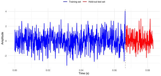
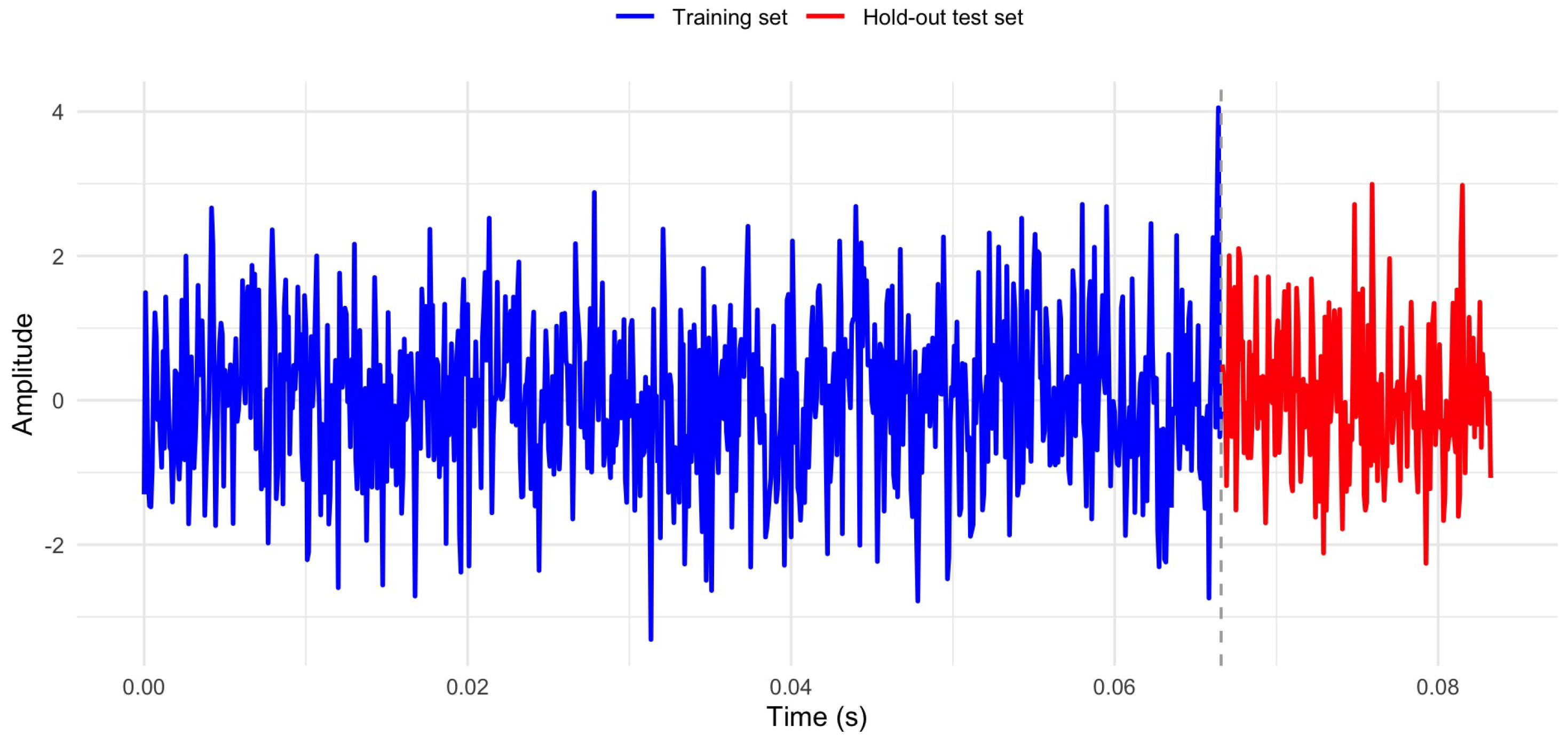
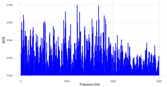
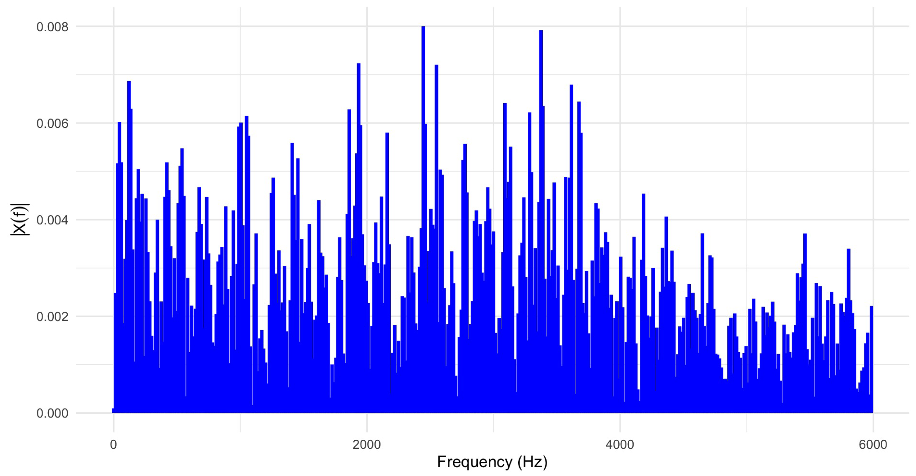
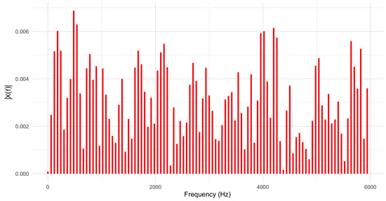
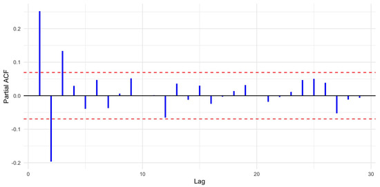
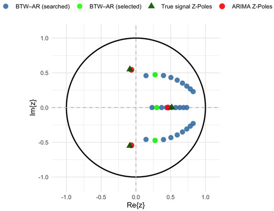
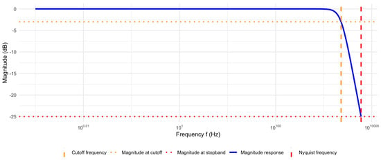
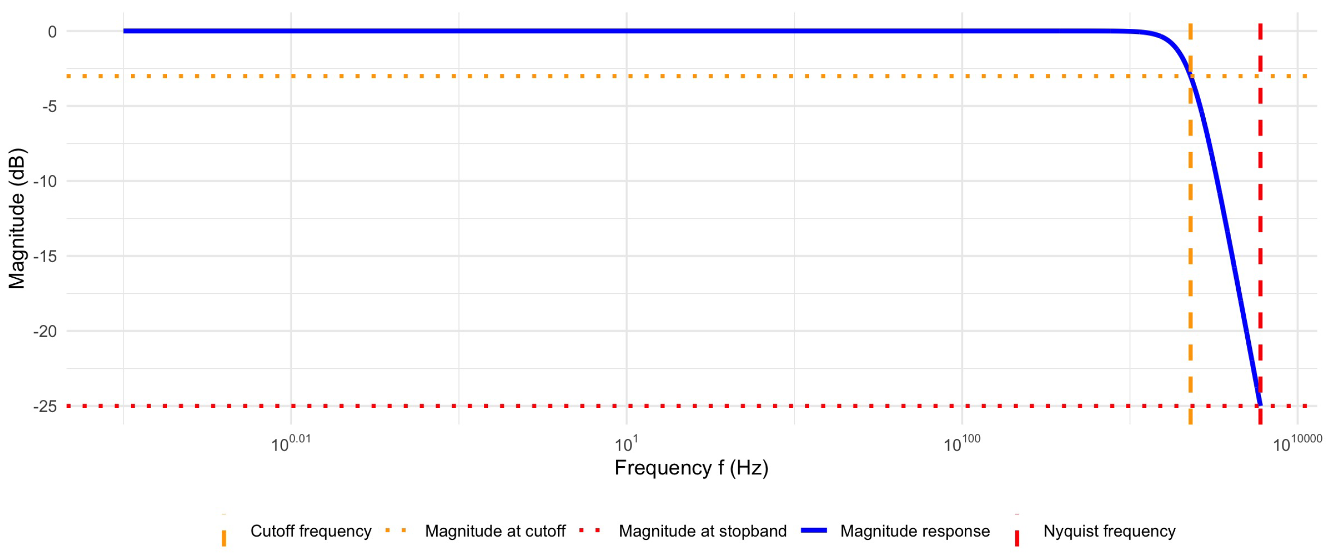
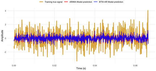
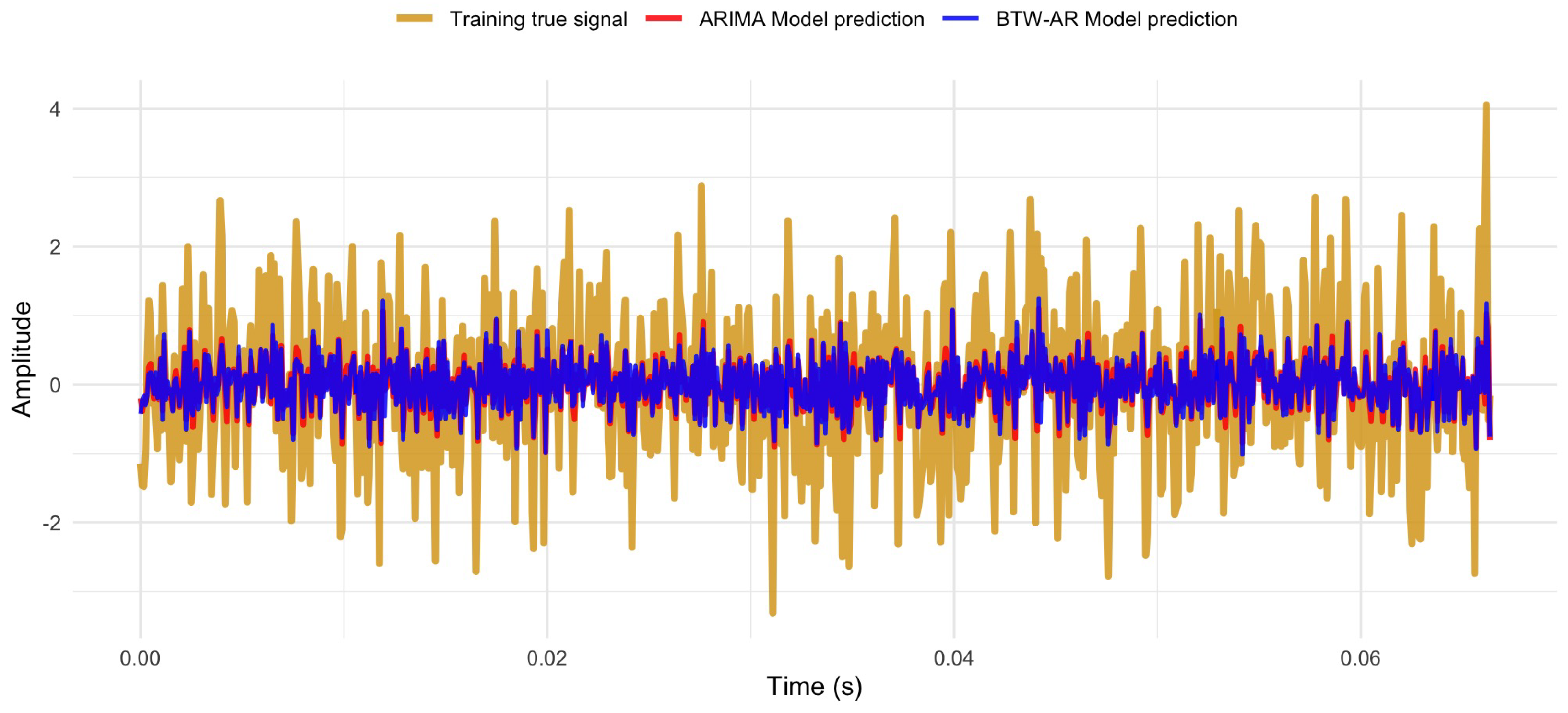
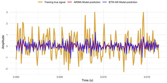
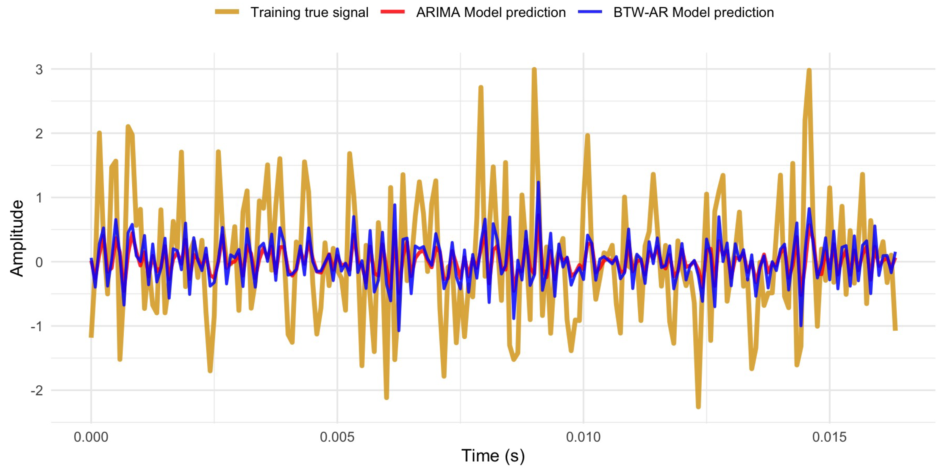
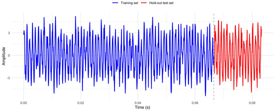
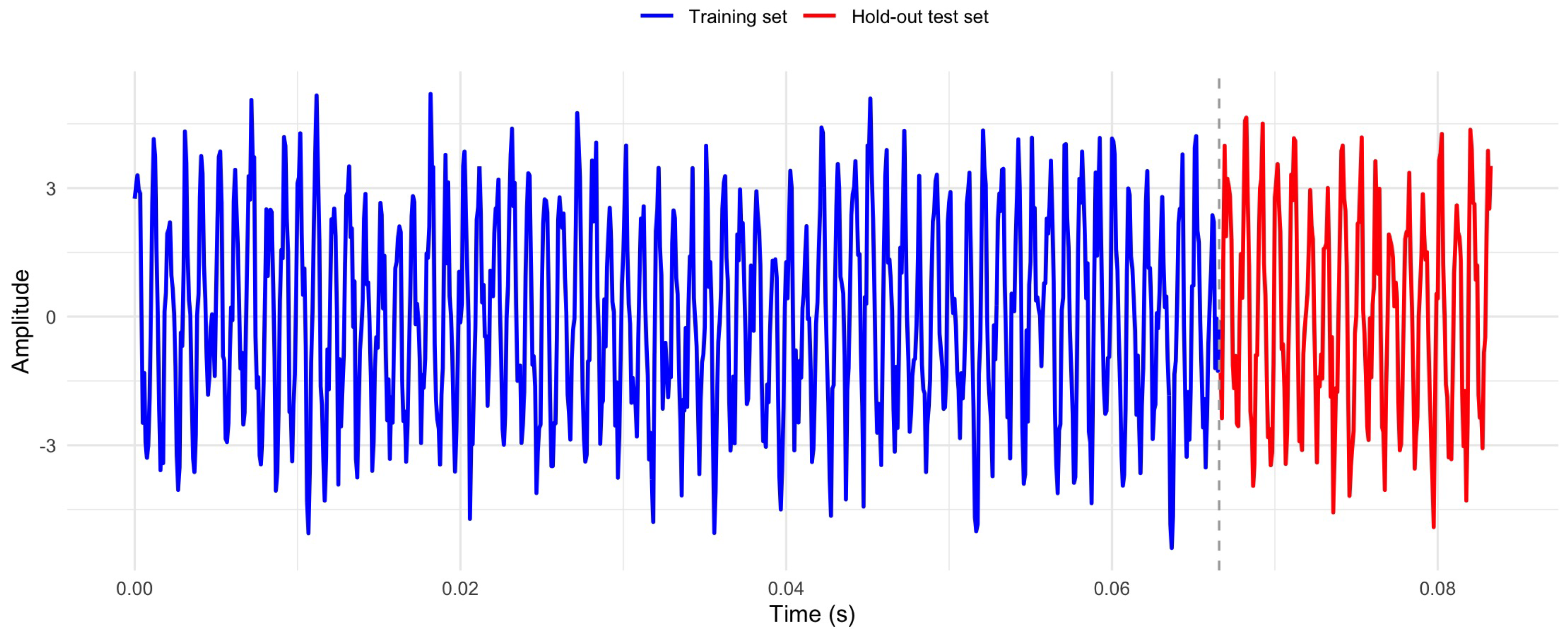
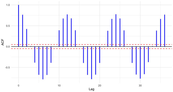
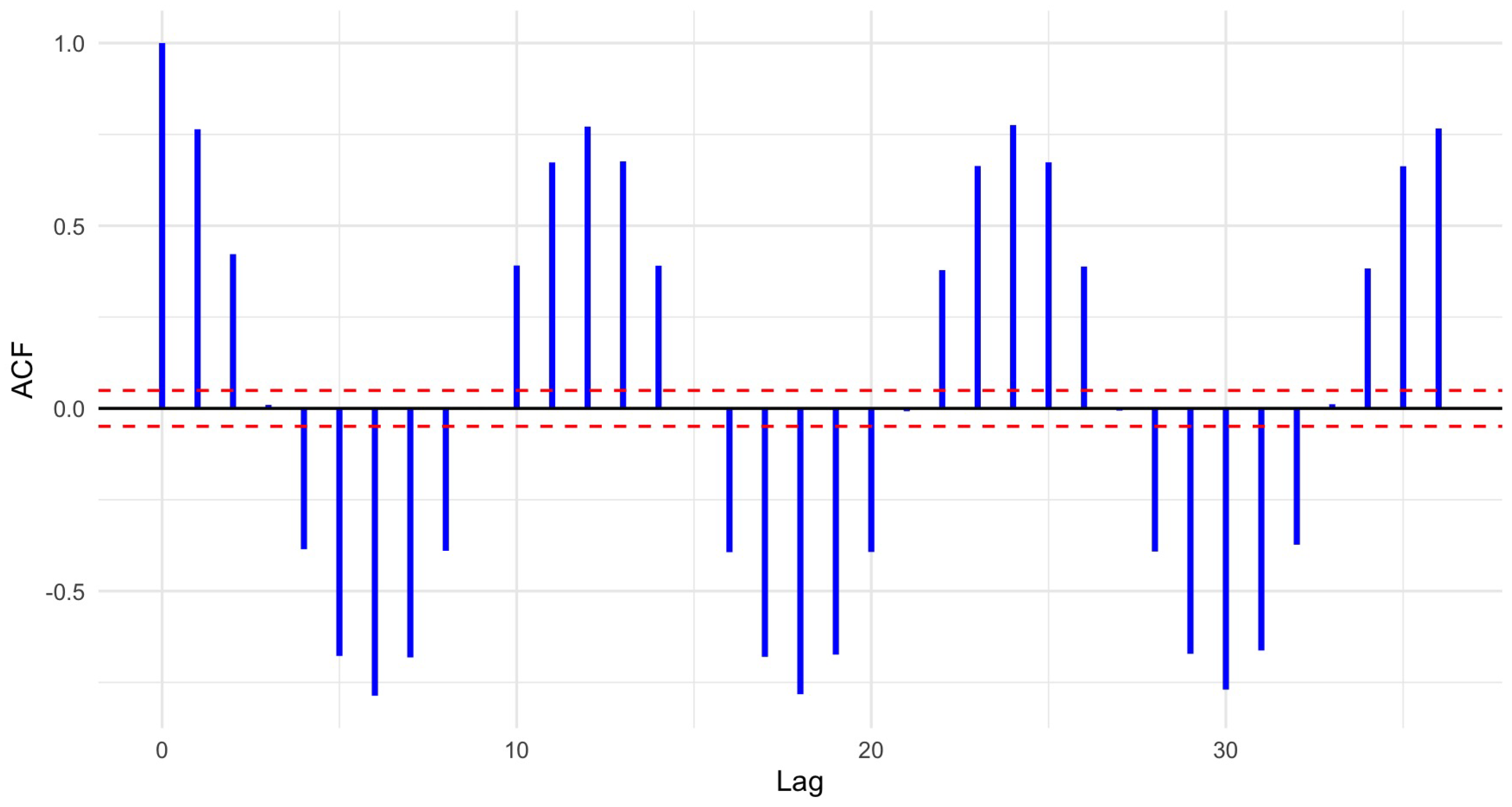
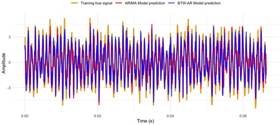
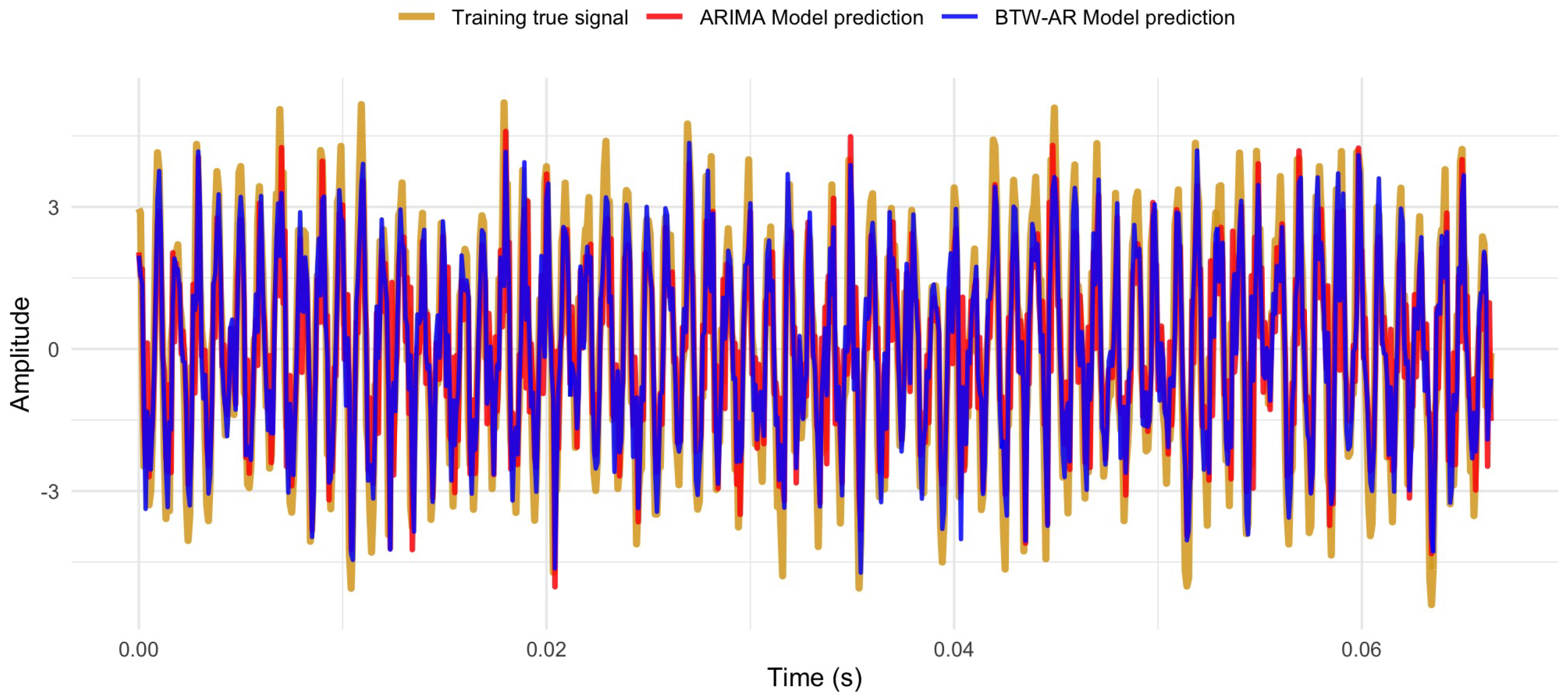
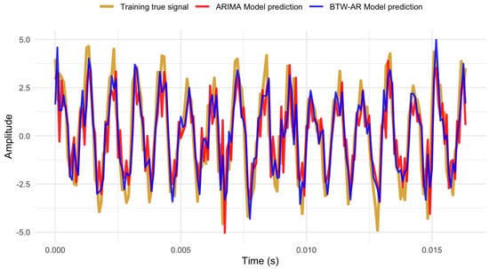
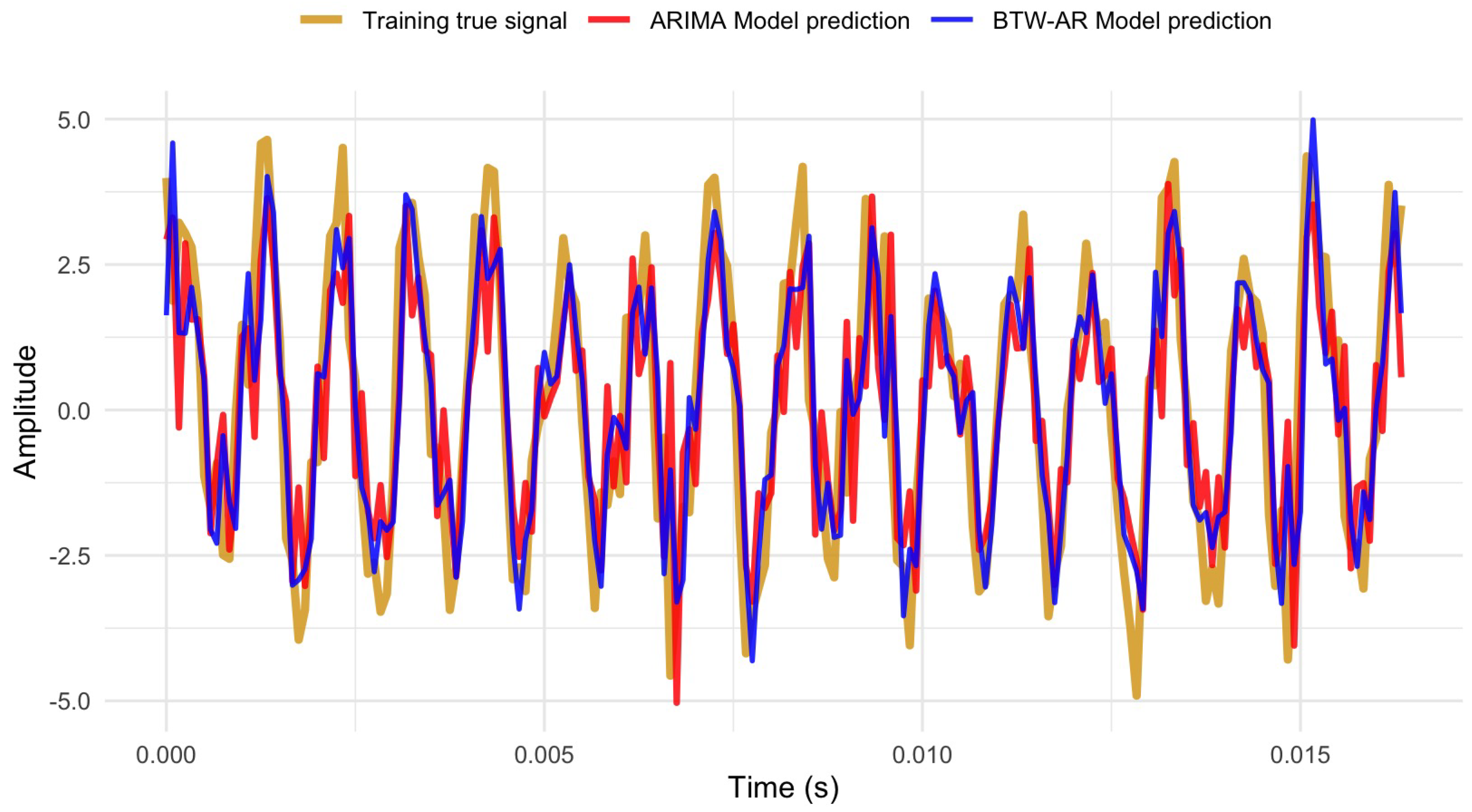
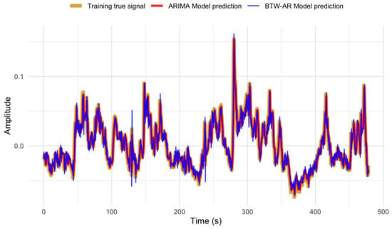
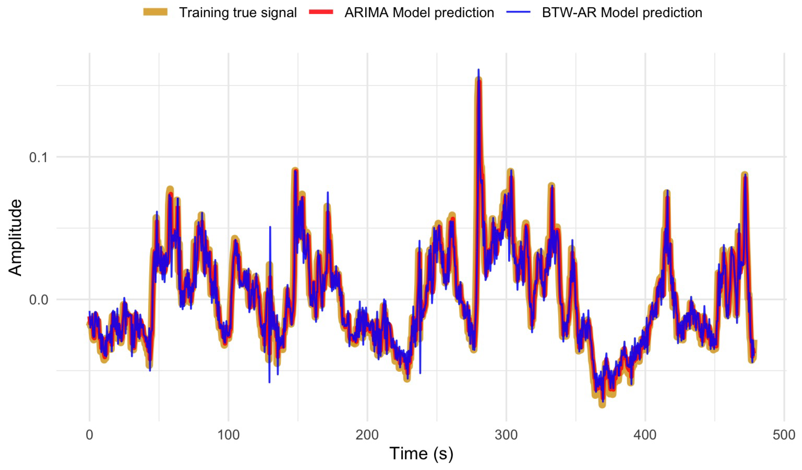
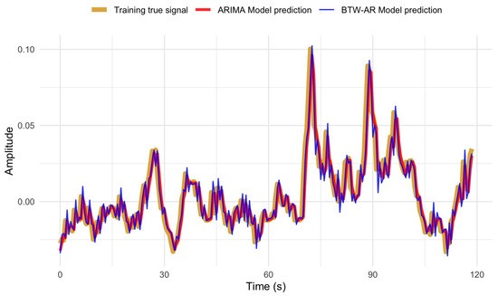
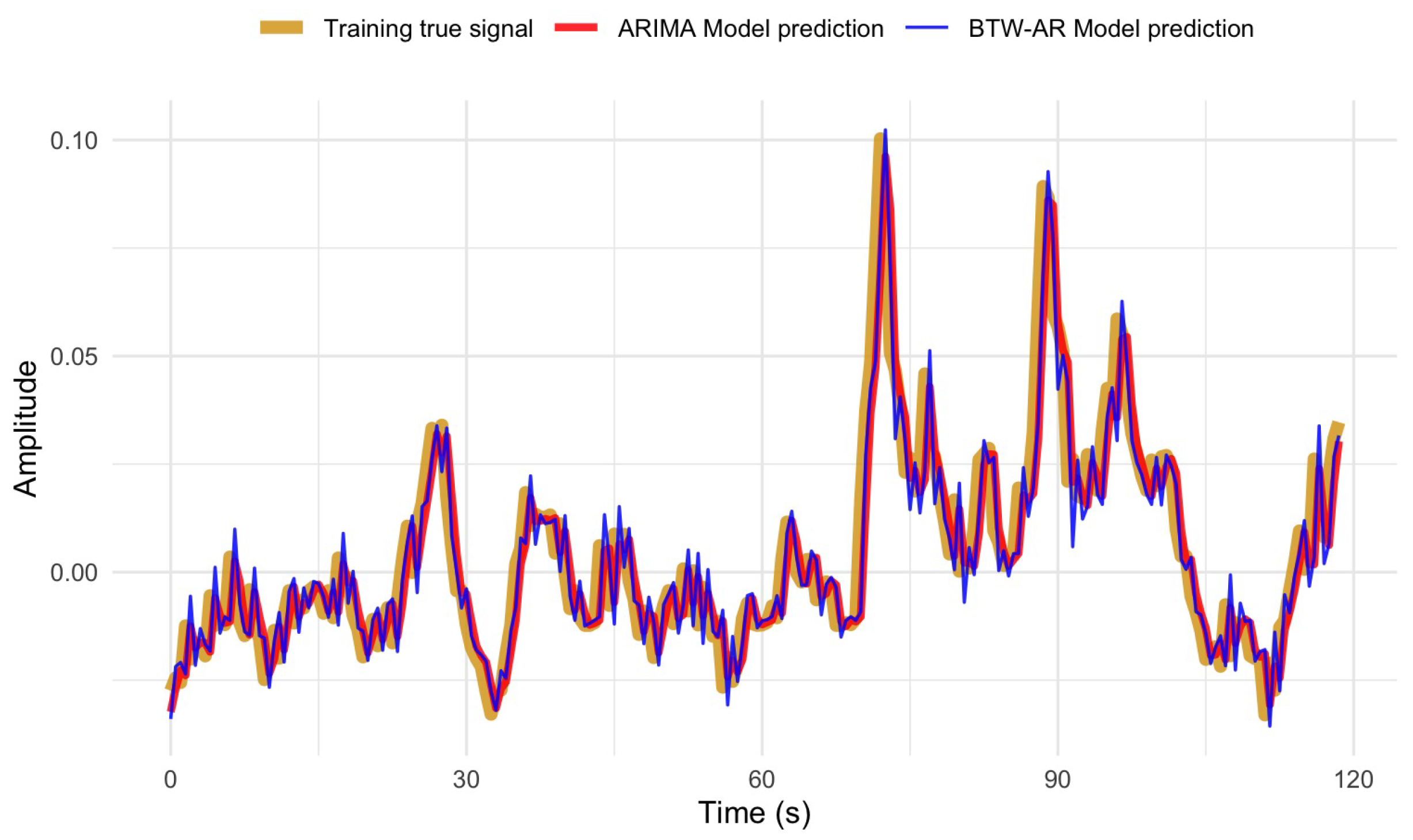
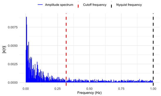
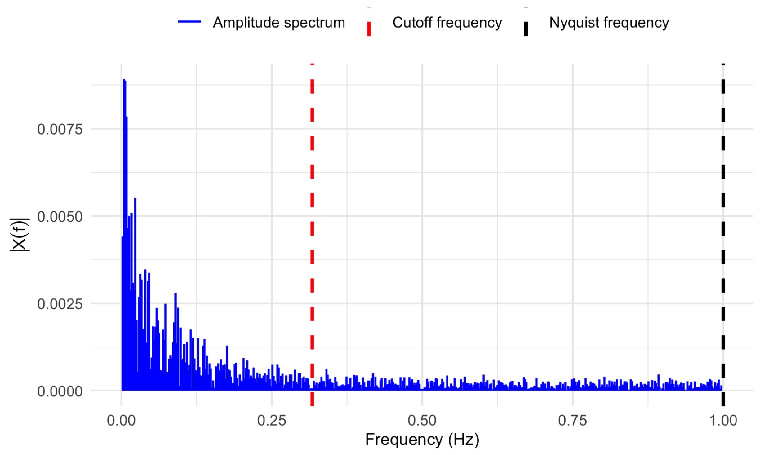
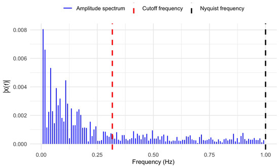
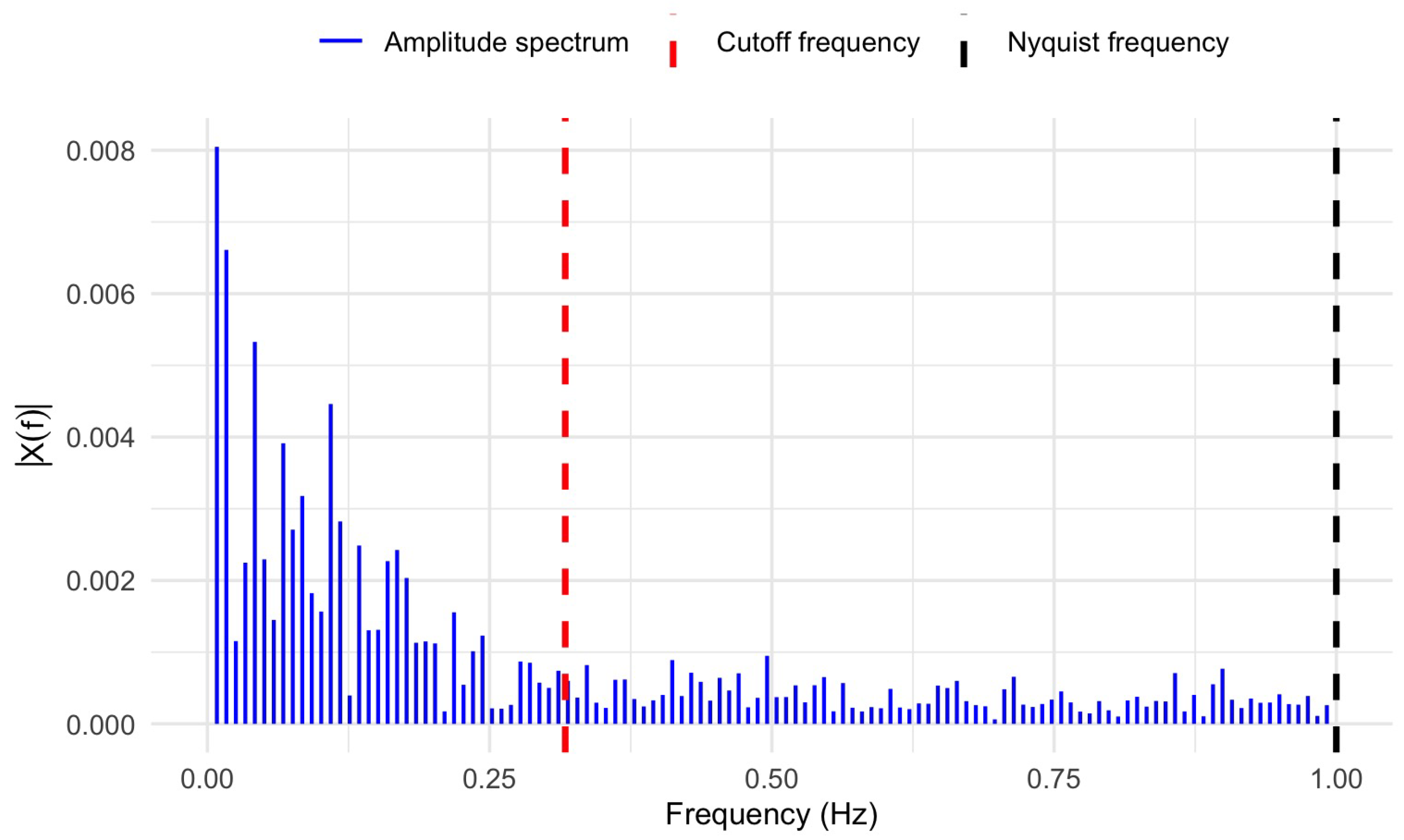

Disclaimer/Publisher’s Note: The statements, opinions and data contained in all publications are solely those of the individual author(s) and contributor(s) and not of MDPI and/or the editor(s). MDPI and/or the editor(s) disclaim responsibility for any injury to people or property resulting from any ideas, methods, instructions or products referred to in the content. |
© 2026 by the authors. Licensee MDPI, Basel, Switzerland. This article is an open access article distributed under the terms and conditions of the Creative Commons Attribution (CC BY) license.